Evaluating Two Optical Methods of Woody-to-Total Area Ratio with Destructive Measurements at Five Larix gmelinii Rupr. Forest Plots in China

Abstract

Accurate in situ leaf area index (LAI) estimates of forest plots are required to validate currently-used LAI map products. Woody-to-total area ratio ($\alpha$) is a crucial parameter in converting the plant area index estimates of forest plots obtained by optical methods into LAI. Although optical methods for estimating the $\alpha$ of forest canopy have been proposed, their performance has never been assessed. In this study, five Larix gmelinii Rupr. forest plots with contrasting plot characteristics (i.e., tree age, tree height, management activities, stand density, and site conditions) were selected. The performance of two commonly used optical methods, namely, multispectral canopy imager (MCI) and digital hemispherical photography (DHP), in estimating the $\alpha$ of L. gmelinii forest plots was evaluated by using the reference $\alpha$ of the selected forest plots. The reference $\alpha$ of forest plots was measured via destructive method by harvesting two or three representative trees in each plot. Large variations were observed amongst the reference $\alpha$ of the selected forest plots (ranging from 0% to 56%). These $\mathsf{\alpha }$ were also highly correlated with the site conditions and management activities in these plots. The effective $\alpha$ (${\alpha }_e$) or $\alpha$ estimated using the leaf-on and leaf-off periods MCI or DHP images with or without consideration of the clumping effects of canopy element and woody components were 1.57 to 4.63 times the reference $\alpha$ in the five plots. The overestimation of $\alpha$ or ${\alpha }_e$ was mainly caused by the preferential shading of woody components by the shoots in the leaf-on canopy. Accurate $\alpha$ estimates for the L. gmelinii forest plots with errors of less than 20% can be obtained from MCI when the clumping effects of canopy element and woody components are considered in the estimation.

1. Introduction

Leaf area index (LAI) is typically used in many models to describe vegetation–atmosphere interactions as crucial variable controlling processes, such as photosynthesis, respiration, and rain interception [1]. LAI is defined as half of the total green leaf area per unit of the flat ground area [2,3]. LAI can be measured in situ and retrieved from remote sensing images. In situ LAI measurements usually provide LAI estimates at the plot scale (e.g., 20 × 20–100 × 100 m). By contrast, LAI maps provide LAI estimates at the regional, national and global scales. Over the past two decades, several commonly used LAI map products have been published, including CYCLOPES [4], GLOBCARBON [5], GLASS [6], MODIS [7], and GEOV1 [8]. However, several studies highlighted huge differences amongst these products [9,10,11,12]. Therefore, accurate and reliable in situ LAI measurements are needed to assess and improve the accuracy of these products and for them to match the accuracy requirements of several applications, such as the Global Climate Observing System (GCOS). The GCOS has specified that LAI map product values must be within 20% of in situ LAI measurements and be improved to within 5% for future applications [1,13].

Methods for estimating in situ LAI measurements can be categorized into direct and indirect methods. On the one hand, direct methods are time consuming, laborlabor-intensive and can sometimes be destructive to canopies [14]. On the other hand, indirect methods are widely used for estimating in situ LAI of vegetation canopies due to their high efficiency, low cost, and nondestructiveness [15]. Amongst these methods, the optical ones are most commonly used, including digital hemispherical photography (DHP), LAI-2000/LAI-2200 (Li-Cor, Lincoln, NE, USA), tracing radiation and architecture of canopies (TRAC) (3rd Wave Engineering, Winnipeg, Manitoba, Canada), HemiView (Dynamax, Houston, TX, USA), SunScan (Delta-T Devices, Cambridge, UK), multispectral canopy imager (MCI) [14], and multiband vegetation imager (MVI) [15]. In situ LAI measurements can be estimated based on the gap fraction or radiation attenuation measurements collected by using optical methods. For forests, the gap fraction or radiation attenuation measurements collected by optical methods include the contribution of leaves or shoots and woody components (e.g., stems, branches, flowers, and fruits). Therefore, the estimates derived from indirect methods are plant area index (PAI) instead of LAI. PAI is the sum of LAI and woody area index (WAI). Optical methods require a parameter called woody-to-total area ratio ($\alpha =WAI/PAI$) [16] to convert PAI into LAI.

The direct method estimates the $\alpha$ of forest canopies by directly measuring the $\mathsf{\alpha }$ of several representative trees in the plots via destructive methods [16]. However, this method is labor-intensive and time-consuming and has been rarely used in practice [14]. The indirect methods for estimating the $\alpha$ of forest canopies mainly include optical methods, such as LAI-2000/LAI-2200 [17,18], DHP [19,20], MCI [14], and MVI [21]. Amongst these methods, LAI-2000/LAI-2200 and DHP estimate the $\alpha$ of forest canopies based on the gap fraction or radiation attenuation measurements collected at leaf-on and leaf-off periods [17,18,19,20]. Meanwhile, the effective WAI ($WA{I}_e$) obtained from LAI-2000/LAI-2200 or DHP at leaf-off period forest canopies is represented as the $WA{I}_e$ of leaf-on period forest canopies in estimating $\alpha$ [17,18,19]. Other studies have estimated the $\alpha$ of forest canopies by calculating the ratio of pixel numbers between woody components and the sum of leaves or shoots and woody components in a group of single-channel DHP images [13,22]. However, these traditional optical methods are unable to discriminate leaves or shoots, branches, stems, fruits and sky. Two multispectral canopy imaging devices (i.e., MVI and MCI) have been developed and applied to estimate $\alpha$ based on the special spectral characteristics of canopy element at visible (VIS) and near-infrared (NIR) bands [14,21]. Previous studies have reported a wide range and relatively large values of $\alpha$ (ranging from 0.03 to 0.41) [14,17,18,23,24]. Therefore, ignoring $\alpha$ can result in approximately 3% to 40% estimation errors in LAI estimates obtained by optical methods. Thus, $\alpha$ must be considered in the in situ LAI estimation of forest canopies.

Although several optical methods have been developed for estimating the $\alpha$ of forest canopies, no study has evaluated the estimation performance of those methods. Moreover, three aspects of those methods require further investigation. Firstly, a constant $\alpha$ value is often used in estimating the LAI of forest plots with the same tree species [16,25]. However, the variations in the $\alpha$ of plots with the same tree species yet varying stand densities, tree ages, site conditions and management activities are often ignored and whether such variations can be accepted for obtaining accurate in situ LAI measurements is yet to be verified. Secondly, for most natural forest canopies, the spatial distribution of the canopy element and woody components in the space largely deviates from the random distribution assumed by the inversion models used by optical methods. Zou et al. reported that the most effective plant area index ($PA{I}_e$) and $WA{I}_e$ estimates derived from optical methods are 35% to 75% and 63% to 90% of the PAI and WAI of leaf-on and leaf-off forest scenes, respectively [15]. Therefore, the clumping effects of canopy element and woody components should be considered in estimating the PAI and WAI of forest canopies. However, no study has evaluated how the clumping effects of canopy element and woody components influence the $\alpha$ estimation of forest plots. Thirdly, several optical methods have been developed for estimating the $\alpha$ of forest canopies. Some studies have attempted to cross-compare the $\mathsf{\alpha }$ estimates obtained by different optical methods [19,20]. However, to the best of our knowledge, no study has attempted to validate the estimation performance of those methods based on the $\alpha$ estimates obtained by direct methods, such as the destructive method.

In this study, five permanent Larix gmelinii Rupr. plots, with varying tree ages, tree heights, stand densities, and site conditions, were selected as elementary sampling units to validate LAI map products. The reference $\alpha$ of each plot was obtained by using the destructive method and the variations amongst the $\alpha$ the five selected forest plots were analyzed. Two classical optical methods (i.e., MCI and DHP) were used to simultaneously estimate the $\alpha$ of these five sites. Factors that affect the estimation performance of MCI and DHP to estimate the $\alpha$ forest plots were analyzed, including inversion model and the clumping effects of canopy element and woody components. The $\alpha$ estimates derived from DHP and MCI were compared with those obtained by the destructive method. The performance of these two optical methods was evaluated afterwards to determine the best method for estimating the $\alpha$ of L. gmelinii forest plots.

2. Theory

2.1. Effective PAI ($PA{I}_e$), Effective WAI ($WA{I}_e$), PAI, and WAI

The PAI of leaf-on forest canopies can be estimated by inverting Beer’s law based on the gap fraction measurements [15,26,27] as follows

$$\mathrm{PAI}=\frac{-ln\left(p_e\left(\theta \right)\right)cos\left(\theta \right){\gamma }_e}{G_e\left(\theta \right){\Omega }_e\left(\theta \right)}$$

(1)

where $p_e\left(\theta \right)$, $G_e\left(\theta \right)$, and ${\Omega }_e\left(\theta \right)$ are the canopy element gap fraction, canopy element projection coefficient and canopy element clumping index (${\Omega }_e$) at zenith angle $\theta$. ${\gamma }_e$ is the needle-to-shoot area ratio for quantifying the effect of needle clumping within a shoot.

Previous studies have reported that the $G_e\left(\theta \right)$ of leaf-on forest canopy is approximately intersected at the zenith angle near 57.3° and can be assumed to be equal to 0.5 at such zenith angle [13,15,28]. Therefore, many studies have attempted to estimate the LAI and PAI of forest canopies based on the Beer’s law and gap fraction measurements collected at this zenith angle or the narrow zenith angle ranges near 57.3° [13,15,27,29,30]. The PAI of leaf-on forest canopies can be calculated based on Equation (1) as follows (57.3)

$$PA{I}_{57.3}=-2ln\left(p_e\left(57\right)\right)cos\left(57\right){\gamma }_e/{\Omega }_e\left(57\right)$$

(2)

where $p_e\left(57\right)$ and ${\Omega }_e\left(57\right)$ denote the canopy element gap fraction measurements and the ${\Omega }_e$ estimates obtained at zenith angle 57° or the narrow zenith angle ranges near 57°, respectively.

Aside from Beer’ law, the PAI of leaf-on forest canopies can be estimated based on Miller theory [31] without prior knowledge of $G_e\left(\theta \right)$ (Miller):

$$PA{I}_{Miller}=-2{{\displaystyle \int }}_0^{\frac{\pi }{2}}\frac{ln\left[p_e\left(\theta \right)\right]{\gamma }_e}{{\Omega }_e\left(\theta \right)}cos\left(\theta \right)sin\left(\theta \right)d\theta$$

(3)

Based on the gap fraction measurements collected from the five annuli of LAI-2000/LAI-2200, a modified Miller theory was used to estimate the PAI of leaf-on forest canopies [15,32] (LAI-2200):

$$PA{I}_{LAI-2200}=-{\displaystyle \sum }_{i=1}^5\frac{ln[p_{e\_i}\left({\theta }_i\right)]{\gamma }_{e}cos\left({\theta }_i\right)W_i}{G_{e\_i}{\Omega }_{e\_i}}$$

(4)

where ${\theta }_i$ is the center zenith angle of the ith annulus and $p_{e\_i}\left({\theta }_i\right)$, $G_{e\_i}$, and $W_i$ are the canopy element gap fraction, canopy element projection coefficient, and weight factor of the ith annulus, respectively. ${\Omega }_{e\_i}$ and ${\mathrm{G}}_{\mathrm{e}\_\mathrm{i}}$ were calculated by averaging the ${\Omega }_e\left(\theta \right)$ and $G_e\left(\theta \right)$ estimates with the zenith angles covered by the ith annulus, respectively. The zenith angle ranges of the five annuli of LAI-2000/LAI-2200 were 0–13°, 16–28°, 32–43°, 47–58° and 61–74°, respectively [15,32]. $W_i$ can be calculated as follows

$$W_i=sin\left({\theta }_i\right)d{\theta }_i$$

(5)

When normalised to 1.0, the values of $W_i$ in Equation (5) were computed as 0.041, 0.131, 0.201, 0.29, and 0.337, which correspond to the five annuli with center zenith angles of 7°, 23°, 38°, 53°, and 68°, respectively [15].

The modified Miller theory also can be adopted by MCI to estimate the PAI of leaf-on forest canopies (MCI_0-85) as follows

$$PA{I}_{MC{I}_0-85}=-{\displaystyle \sum }_{i=1}^9\frac{ln\left[P_{e\_i}\left({\theta }_i\right)\right]{\gamma }_{e}cos\left({\theta }_i\right)W_i}{G_{e\_i}{\Omega }_{e\_i}}$$

(6)

By using Equation (5), the $W_i$ for the nine annuli of MCI were computed as 0.0038, 0.0303, 0.0596, 0.0872, 0.1120, 0.1335, 0.1510, 0.1640, and 0.2750 whilst the zenith angle ranges covered by these annuli were 0–5°, 5–15°, 15–25°, 25–35°, 35–45°, 45–55°, 55–65°, 65–75°, and 75–85°.

If the beyond- (${\Omega }_e$) and within-shoot clumpings (${\gamma }_e$) are not considered in estimating the PAI of leaf-on forest canopies (where ${\Omega }_e\left(\theta \right)$, ${\Omega }_e\left(57\right)$, ${\Omega }_{e\_i}$, and ${\gamma }_e$ are assumed to be equal to 1, then the estimates derived from Equations (2), (3), (4), and (6) are $PA{I}_{e\_57.3}$, $PA{I}_{e\_Miller}$, $PA{I}_{e\_LAI-2200}$, and $PA{I}_{e\_MCI\_0-85}$, respectively. Given that the spatial distribution of the canopy element for most natural forest canopies usually deviates from the random distribution. Optical methods usually fail in detecting small gaps between needles within shoots [14,33]. Therefore, both ${\Omega }_e$ and ${\gamma }_e$ should be considered in estimating the PAI of leaf-on forest canopies. Several algorithms have been developed to estimate the ${\Omega }_e$ and woody components clumping index (${\Omega }_w$) of leaf-on and leaf-off forest canopies, including logarithmic averaging (LX) [34], modified logarithmic averaging (LXW) [35], gap size distribution (CC) [36,37], modified gap size distribution (CMN) [38], combination of gap size and logarithmic averaging (CLX) [39], and Pielou’s coefficient of spatial segregation (PCS) [40]. Previous studies show that PCS tend to produce error ${\mathsf{\Omega }}_{\mathrm{e}}$ and ${\mathsf{\Omega }}_{\mathrm{w}}$ estimates [15,35,38]. Moreover, high similarities are observed between CC and CMN as well as between LX and LXW [15]. For conciseness, only the three algorithms of CC, LX and CLX recommended by Zou et al. [15] were used in this study. Table 1 presents the ${\Omega }_e$ and ${\gamma }_e$ estimation formulae used in this study.

Table 1. The ${\Omega }_e$ and ${\gamma }_e$ estimation formulae used in this study. $F_m\left(0,\theta \right)$ is the measured total gap fraction of the canopy element at zenith angle $\theta$ (i.e., accumulated gap fraction from the largest to the smallest gaps), $F_{mr}\left(0,\theta \right)$ is the total gap fraction after removing those large gaps resulting from the nonrandom distribution of the canopy element [14,36,41], $\overline{p_e\left(\theta \right)}$ is the mean canopy element gap fraction of all segments at $\theta$, $\overline{ln\left[p_e\left(\theta \right)\right]}$ is the mean logarithmic canopy element gap fraction for all segments at $\theta$ [34,41], $n$ is the number of segments, $p_{e\_k}\left(\theta \right)$ is the canopy element gap fraction of segment $k$, ${\Omega }_{e\_CC\_k}\left(\theta \right)$ is the ${\Omega }_e$ of segment $k$ at $\theta$ estimated by CC [35,39], and $A_n$ is half of total needle area in a shoot. $A_p\left(0°,0°\right)$, $A_p\left(45°,0°\right)$, and $A_p\left(90°,0°\right)$ are the shoot projection areas measured by projecting the shoot at zenith angles 0°, 45°, and 90° and azimuth angle 0°, respectively [16]. $\gamma$ is the effective needle-to-shoot area ratio derived based on the $A_p\left(0°,0°\right)$, $A_p\left(45°,0°\right)$, $A_p\left(90°,0°\right)$, and $A_n$ of each shoot sample. ${\gamma }_e$ is the needle-to-shoot area ratio that corrects the overestimation of $\gamma$ for woody components in estimating the PAI of leaf-on forest canopies [14].

Equation		References
${\Omega }_{e\_CC}\left(\theta \right)=\frac{ln\left(F_m\left(0,\theta \right)\right)}{ln\left(F_{mr}\left(0,\theta \right)\right)}\ast \left[1+\frac{F_m\left(0,\theta \right)-F_{mr}\left(0,\theta \right)}{1-F_m\left(0,\theta \right)}\right]$	(7)	[36]
${\Omega }_{e\_LX}\left(\theta \right)=\frac{ln\left[\overline{p_e\left(\theta \right)}\right]}{\overline{ln\left[p_e\left(\theta \right)\right]}}$	(8)	[34]
${\Omega }_{e\_CLX}\left(\theta \right)=\frac{nln\left[\overline{p_e\left(\theta \right)}\right]}{{{\displaystyle \sum }}_{k=1}^{n}ln\left[p_{e\_k}\left(\theta \right)\right]/{\Omega }_{e\_CC\_k}\left(\theta \right)}$	(9)	[39]
$\gamma =\frac{A_n}{\frac{A_p\left(0°,0°\right)\ast cos\left(15°\right)+A_p\left(45°,0°\right)\ast cos\left(45°\right)+A_p\left(90°,0°\right)\ast cos\left(75°\right)}{cos\left(15°\right)+cos\left(45°\right)+cos\left(75°\right)}}$	(10)	[16]
${\gamma }_e=1\ast \frac{WAI}{PAI}+\gamma \ast \left[PAI-WAI\right]/PAI$	(11)	[14]

In this study, the equations used for estimating $WA{I}_{e\_57.3}$, $WA{I}_{e\_Miller}$, $WA{I}_{e\_LAI-2200}$, $WA{I}_{e\_MCI\_0-85}$, $WA{I}_{57.3}$, $WA{I}_{Miller}$, $WA{I}_{LAI-2200}$, and $WA{I}_{MCI\_0-85}$ of leaf-off forest canopies are the same as those used for estimating $PA{I}_{e\_57.3}$, $PA{I}_{e\_Miller}$, $PA{I}_{e\_LAI-2200}$, $PA{I}_{e\_MCI\_0-85}$, $PA{I}_{57.3}$, $PA{I}_{Miller}$, $PA{I}_{LAI-2200}$, and $PA{I}_{MCI\_0-85}$, respectively. Similarly, the equations used for estimating ${\Omega }_{w\_CC}\left(\theta \right)$, ${\Omega }_{w\_LX}\left(\theta \right)$, and ${\Omega }_{w\_CLX}\left(\theta \right)$ of leaf-off forest canopies are the same as those used for estimating ${\Omega }_{e\_CC}\left(\theta \right)$, ${\Omega }_{e\_LX}\left(\theta \right)$ and ${\Omega }_{e\_CLX}\left(\theta \right)$, respectively.

2.2. Effective Woody-to-Total Area Ratio (${\alpha }_e$) and Woody-to-Total Area Ratio ($\alpha$)

If ${\Omega }_e$ and ${\Omega }_w$ are not considered in estimating the $\alpha$ of leaf-on forest canopies, then the estimates derived from optical methods are computed as ${\alpha }_e$ (effective woody-to-total area ratio) [14,19,42]:

$${\alpha }_e=\raisebox{1ex}{$WA{I}_e$}\!\left/ \!\raisebox{-1ex}{$PA{I}_e$}\right.$$

(12)

Sea et al. [22] proposed another method to estimate the ${\alpha }_e$ of leaf-on forest canopies based on the canopy and woody component cover fractions ($f_c$ and $f_w$) as follows (percentage)

$${\alpha }_e=\raisebox{1ex}{$f_w$}\!\left/ \!\raisebox{-1ex}{$f_c$}\right.$$

(13)

where $f_c$ is the ratio of the total pixel numbers of leaves or shoots and woody components to the pixel number of the classified DHP or MCI images, whereas $f_w$ is the ratio of the pixel number of woody components to the pixel number of classified DHP or MCI images [13,22].

If ${\Omega }_e$ and ${\Omega }_w$ are considered in estimating the $\alpha$ of leaf-on forest canopies, then $\alpha$ can be estimated as follows

$$\alpha =\raisebox{1ex}{$WAI$}\!\left/ \!\raisebox{-1ex}{$PAI$}\right.$$

(14)

where PAI and WAI are were obtained from DHP or MCI.

For the destructive method, harvesting all trees in each forest plot is impossible, especially for those plots that have been established as long-term observation plots for validating LAI map products. Some studies have attempted to estimate the $\alpha$ of forest plots based on the $\alpha$ of several harvested trees located in or nearby these plots [16,23,43]. This study also applied such method to estimate the $\alpha$ of forest plots based on the $\alpha$ of destructive trees and the basal area of the trees in these plots:

$$\alpha =\frac{B_d}{B_d+B_c+B_s}{\alpha }_d+\frac{B_c}{B_d+B_c+B_s}{\alpha }_c+\frac{B_s}{B_d+B_c+B_s}{\alpha }_s$$

(15)

where $B_d$, $B_c$, and $B_s$ are the basal area of the dominant, codominant and suppressed trees in the plots, respectively; and ${\alpha }_d$, ${\alpha }_c$ and ${\alpha }_s$ are the estimated $\alpha$ of the representative dominant, codominant, and suppressed trees as measured by the destructive method, respectively.

3. Materials and Methods

3.1. Plots Description

The five forest plots selected in this study are located in the Saihanba National Forest Park in Hebei Province, China (Figure 1). These plots are monocultural with a flat terrain and a size of 25 m × 25 m. Forest inventories were carried out during the LAI measurement campaign (Table 2). For plots 1 and 2, the majority of the branches below the live canopies were harvested during the selective thinning performed in the winter of 2014. For plots 3 and 4, the dead branches with heights of less than about 2.5 m were low- and medium-level harvested before the LAI measurement campaign, respectively. For plot 5, all branches of forest canopies were not harvested before the LAI measurement campaign.

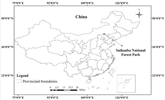
Figure 1. Location of the Saihanba National Forest Park in Hebei Province, China.

Table 2. Characteristics of Larix gmelinii Rupr. plots.

	Plot 1	Plot 2	Plot 3	Plot 4	Plot 5
Longitude and latitude	42°24’43” N, 117°19’4” E	42°24’2” N, 117°18’40” E	42°18’2” N, 117°18’9” E	42°25’22” N, 117°19’32” E	42°17’42” N, 117°16’53” E
Mean tree height (m) *	19.43	20.4	12.58	13.31	8.73
Average DBH** (cm)	26.58	27.22	12.71	14.14	9.23
Mean element width (mm)	21.66	23.34	17.91	21.09	17.60
Stand density (stems/ha)	464	384	2320	1760	3904
Tree age (~years)	54	55	21	22	13
Needle-to-shoot area ratio (${\gamma }_e$)	1.30	1.17	1.14	1.17	1.28
Tree species	Larix gmelinii

* The height of trees in each plot was measured based the point cloud dataset collected using the terrestrial laser scanner in the 2017 LAI measurement campaign. The height of each tree was computed as the vertical distance between the highest point of the tree and the lowest point of the stem located close to the ground. ** Diameter at breast height.

3.2. Mean Element Eidth and Needle-to-Shoot Area Ratio (${\gamma }_e$) Measurement

The typical shoots used for measuring the mean element width and needle-to-shoot area ratio were collected by using a ladder at the three height classes of forest canopies (i.e., top, middle and bottom). Two to four shoot samples were randomly obtained at each height class of the five plots. The mean element width of each shoot sample was calculated by using the method described in Leblanc et al. [44]. The mean element width of each plot was derived by averaging the mean element width estimates of all typical shoots in the plot.

The shoot projection areas were recorded by using a Canon 6D camera equipped with a Canon 24–70 mm lens and a flat, levelled white panel with two rulers laid on its top surface. Three shoot projection images were obtained for each shoot by rotating the shoot main axis at zenith angles 0°, 45°, and 90° and azimuth angle 0°. $A_p\left(0°,0°\right)$, $A_p\left(45°,0°\right)$, and $A_p\left(90°,0°\right)$ were obtained for each shoot based on the three shoot projection images. The $A_n$ of each shoot was measured by applying the volume displacement method described in Chen et al. [33]. Afterwards, the $\gamma$ of each typical shoot was calculated by using Equation (10). The $\gamma$ of each plot was estimated by averaging the $\gamma$ of all sampled typical shoots. The ${\gamma }_e$ of each plot was calculated by using Equation (11) based on the $\gamma$ and reference $\alpha$ of the plot.

3.3. DHP Images Acquisition and Processing

A cross-pattern sampling scheme with nine sampling points (with a 5 m distance interval between each sampling point, except for the central sampling point) was used to collect DHP images (Figure 2). The sampling points were marked with wooden stakes to facilitate the two periods collection of leaf-on and leaf-off DHP images at each sampling point. These DHP images were collected by using a Canon 6D camera with a height of about 1.2 m and equipped with a Sigma 8 mm fisheye lens. The DHP images had a resolution of 5472 × 3678 pixels. The exposure parameter was set manually to avoid the overexposure or underexposure of DHP images. All images were collected before sunrise, after sunset, or under an overcast sky. Both leaf-on and leaf-off periods DHP images were collected for each plot (Figure 3a,b, respectively). The leaf-on period DHP images were collected between 11 August and 2 September 2017 at the maximum PAI (maximum LAI) period of the five plots. The leaf-off period DHP images were collected between 28 October and 15 November 2017 at the minimum PAI (equals to WAI and the LAI equals to 0) of the five plots. A total of 90 DHP images were obtained from these plots.

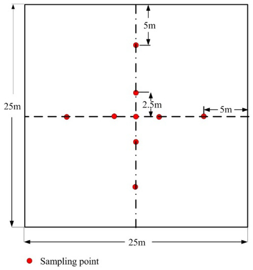
Figure 2. Sampling scheme of the digital hemispherical photography (DHP) method.

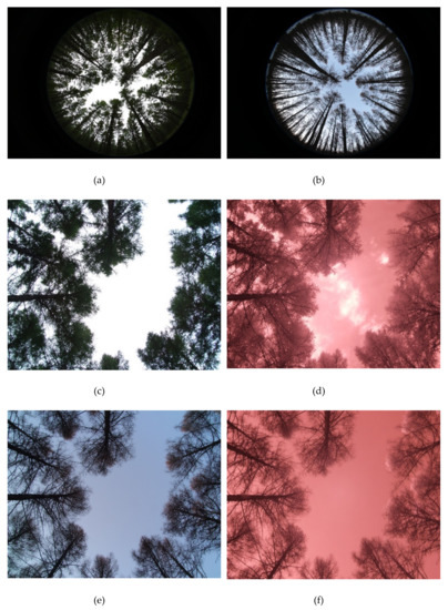
Figure 3. The DHP or multispectral canopy imager (MCI) images collected from the same sampling point or the same sampling point with the same zenith and horizontal angles at leaf-on and leaf-off periods in plot 1. (a) Leaf-on period DHP image, (b) leaf-off period DHP image, (c) leaf-on period visible (VIS) band MCI image, (d) leaf-on period near-infrared (NIR) band MCI image, (e) leaf-off period VIS band MCI image, and (f) leaf-off period NIR band MCI image.

The DHP images were preprocessed by using the same procedure described in Gonsamo and Pellikka [45]. The image preprocessing procedure includes cropping the circular areas of the DHP images, selecting the blue channel, applying a correction for gamma, and thresholding to classify the canopy element and sky. The in-house software called Measurement Tools of Vegetation Structural Parameters (MTVSP, version 2018, Fuzhou, China), which was developed using the MATLAB programming language, was used to calculate the $p_e\left(\theta \right)$, $p_w\left(\theta \right)$, ${\Omega }_e$, ${\Omega }_w$, $WA{I}_e$, $PA{I}_e$, WAI, and PAI of the leaf-on and leaf-off forest plots based on the classified DHP images and MCI image pairs. For the DHP method, the calculation procedures for $p_e\left(\theta \right)$, $p_w\left(\theta \right)$, $p_{e\_i}\left({\theta }_i\right)$, $p_{w\_i}\left({\theta }_i\right)$, $p_e\left(57\right)$, and $p_w\left(57\right)$ were the same as those described in Zou et al. [15]. An assumption of spherical projection function was made for the canopy element ($G_e$) and woody components ($G_w$) projection functions in the PAI and WAI estimation because no $G_e$ and $G_w$ measurements were collected in the field for the five plots.

For the DHP method, six segment sizes were used by LX (5°, 15°, and 30°) and CLX (15°, 30°, and 45°) to estimate the ${\Omega }_e$ and ${\Omega }_w$ of leaf-on and leaf-off forest canopies. The reasons for selecting the six segment sizes are explained in detail in Zou et al. [15]. Seven ${\Omega }_e\left(\theta \right)$ or ${\Omega }_w\left(\theta \right)$ estimates were obtained by using CC, LX, and CLX at each zenith angle ranging from 10° to 90° with a 1° interval at each plot (one estimate for ${\Omega }_{e\_CC}\left(\theta \right)$ or ${\Omega }_{w\_CC}\left(\theta \right)$ and three estimates each for ${\Omega }_{e\_LX}\left(\theta \right)$ and ${\Omega }_{e\_CLX}\left(\theta \right)$ or ${\Omega }_{w\_LX}\left(\theta \right)$ and ${\Omega }_{w\_CLX}\left(\theta \right)$). The ${\Omega }_e\left(\theta \right)$ and ${\Omega }_w\left(\theta \right)$ estimates at 10 zenith angles ranging from of 0° to 9° with a 1° interval were assumed to be equal to ${\Omega }_e\left(10\right)$ and ${\Omega }_w\left(10\right)$, respectively [15]. This assumption was adopted to obtain 91 ${\Omega }_e\left(\theta \right)$ and ${\Omega }_w\left(\theta \right)$ estimates that match the $p_e\left(\theta \right)$ and $p_w\left(\theta \right)$ measurements at the same zenith angle range of 0° to 90° with a 1° interval. The ${\Omega }_{e\_i}$ or ${\Omega }_{w\_i}$ in Equation (4) was calculated by averaging the ${\Omega }_e\left(\theta \right)$ or ${\Omega }_w\left(\theta \right)$ estimates with the zenith angles covered by the ith annulus. The ${\Omega }_e\left(57\right)$ or ${\Omega }_w\left(57\right)$ in Equation (2) was calculated by averaging the ${\Omega }_e\left(\theta \right)$ or ${\Omega }_w\left(\theta \right)$ with zenith angles ranging from 52° to 62° with a 1° interval. Three groups of $PA{I}_e$ and $WA{I}_e$ estimates of $PA{I}_{e\_57.3}$ and $WA{I}_{e\_57.3}$, $PA{I}_{e\_Miller}$ and $WA{I}_{e\_Miller}$, as well as $PA{I}_{e\_LAI-2200}$ and $WA{I}_{e\_LAI-2200}$ were calculated for each plot by using Equations (2) to (4) based on the $p_e\left(\theta \right)$, $p_w\left(\theta \right)$, $p_{e\_i}\left({\theta }_i\right)$, $p_{w\_i}\left({\theta }_i\right)$, $p_e\left(57\right)$, and $p_w\left(57\right)$ measurements. Afterwards, three ${\alpha }_e$ estimates were obtained for each plot by using Equation (12) based on the three groups of $PA{I}_e$ and $WA{I}_e$ estimates. A total of 21 groups of PAI and WAI estimates were calculated for each plot by using Equations (2) to (4) based on the three groups of $PA{I}_e$ and $WA{I}_e$ estimates ($PA{I}_{e\_57.3}$ and $WA{I}_{e\_57.3}$, $PA{I}_{e\_Miller}$ and $WA{I}_{e\_Miller}$, as well as $PA{I}_{e_{LAI}-2200}$ and $WA{I}_{e\_LAI-2200}$) and seven ${\Omega }_e$ and ${\Omega }_w$ estimates derived from the combinations of the three algorithms of CC, LX, and CLX and the four segment sizes of 5°, 15°, 30°, and 45° (seven estimates for each group of PAI and WAI estimates, including $PA{I}_{57.3}$ and $WA{I}_{57.3}$, $PA{I}_{Miller}$ and $WA{I}_{Miller}$, as well as $PA{I}_{LAI-2200}$ and $WA{I}_{LAI-2200}$). Afterwards, 21 $\alpha$ estimates were derived for each plot by using Equation (14) based on 21 groups of PAI and WAI estimates.

3.4. MCI Images Acquisition and Processing

Two representative locations were selected for the collection of MCI images in each plot. The same procedures for collecting MCI image pairs adopted in previous works were used in this study with two key differences [14,41]. Firstly, the MCI image pairs were collected in zenith directions ranging from 0° to 80° with a 10° interval (i.e., nine zenithal measurements at each azimuthal direction). Secondly, the manual exposure model was used to capture MCI images to avoid overexposure and underexposure. The MCI instrument height was about 1.2 m and MCI image resolution was 3488 × 2616 pixels. The MCI measurements were collected before sunrise, after sunset or under an overcast sky. To minimize the effect of forest canopy movement on the collection of MCI image pairs, the MCI measurements were collected under windless or breezy conditions [14,41]. Both leaf-on and leaf-off periods MCI measurements were collected in each plot (Figure 3c–f). The leaf-on period MCI measurements were collected from 20 August to 12 September 2017 at the maximum PAI (maximum LAI) period of the plots. The leaf-off period MCI measurements were collected from October 31 to 16 November 2017 and 4 May 2018 at the minimum PAI (equals to WAI and the LAI equals to 0) of the plots. A total of 1080 MCI image pairs were obtained from the five plots.

The procedures used for processing the MCI image pairs were the same as those described in Zou et al. [14], except that the images were subdivided into two sub-images to reduce the amount of work needed. The MCI image pairs were eventually classified into sky, woody components, and shoots [14]. For the MCI method, $p_e\left(57\right)$ and $p_w\left(57\right)$ were calculated by using the classified MCI images of the seventh annuli collected with a center zenith angle of 60°.

The full size of each pixel of the MCI images was calculated based on the field of view of MCI, image resolution, mean tree height of the plot and the zenith angle where these images were collected [14,21]. The pixel number of the segment required as the key parameter for LX and CLX in the ${\Omega }_e$ and ${\Omega }_w$ estimation of leaf-on and leaf-off forest plots was calculated based on the full size of each pixel of the MCI images. A total of 27 ${\Omega }_e\left(\theta \right)$ or ${\Omega }_w\left(\theta \right)$ estimates were obtained for each annulus of the MCI measurements at the nine zenith angles covered by the annulus with a 1° interval (three estimates each for ${\Omega }_{e\_CC}\left(\theta \right)$, ${\Omega }_{e\_LX}\left(\theta \right)$, and ${\Omega }_{e\_CLX}\left(\theta \right)$ at nine zenith angles). The center zenith angle of the nine zenith angles was defined as the zenith angle where the MCI images were collected. The ${\Omega }_{e\_i}$ or ${\Omega }_{w\_i}$ in Equation (6) was calculated by averaging the nine ${\Omega }_e\left(\theta \right)$ or ${\Omega }_w\left(\theta \right)$ estimates of the i^th annulus. The ${\Omega }_e\left(57\right)$ or ${\Omega }_w\left(57\right)$ in Equation (2) was treated as the ${\Omega }_{e\_i}$ or ${\Omega }_{w\_i}$ estimate of the seventh annulus. Two groups of $PA{I}_e$ and $WA{I}_e$ estimates of $PA{I}_{e\_57.3}$ and $WA{I}_{e\_57.3}$ as well as $PA{I}_{e\_MCI\_0-85}$ and $WA{I}_{e\_MCI\_0-85}$ were calculated for each sampling point by using Equations (2) and (6) based on the $p_{e\_i}\left({\theta }_i\right)$, $p_{w\_i}\left({\theta }_i\right)$, $p_e\left(57\right)$, and $p_w\left(57\right)$ measurements. Two ${\alpha }_e$ estimates were calculated for each sampling point by using Equation (12) based on the two groups of $PA{I}_e$ and $WA{I}_e$ estimates. The ${\alpha }_e$ of each plot was calculated by averaging the ${\alpha }_e$ of the two sampling points. Six groups of PAI and WAI estimates were calculated for each plot by using Equations (2) and (6) based on the two groups of $PA{I}_e$ and $WA{I}_e$ estimates ($PA{I}_{e\_57.3}$ and $WA{I}_{e\_57.3}$ as well as $PA{I}_{e\_MCI\_0-85}$ and $WA{I}_{e\_MCI\_0-85}$) and the three ${\Omega }_e$ and ${\Omega }_w$ estimates derived from CC, LX, and CLX (three estimates each for group $PA{I}_{57.3}$ and $WA{I}_{57.3}$ as well as $PA{I}_{MCI\_0-85}$ and $WA{I}_{MCI\_0-85}$). Six $\alpha$ estimates were obtained for each plot by using Equation (14) based on the six groups of PAI and WAI estimates.

Classifying the leaf-on period DHP images into sky, shoot, and woody components by using the method described in Sea et al. [22] entails a large uncertainty. Therefore, the classified leaf-on period MCI images were used to estimate the ${\alpha }_e$ of leaf-on forest plots if the percentage method was adopted. The $f_c$ or $f_w$ was calculated by taking the ratio of the sum of the canopy element or woody components pixels to the sum of the image pixel number of the classified leaf-on period MCI images. Afterwards, the ${\alpha }_e$ of each sampling position was calculated by using Equation (15) based on the obtained $f_c$ and $f_w$ estimates. The ${\alpha }_e$ of each plot was then calculated by averaging the two ${\alpha }_e$ estimates of the two sampling points.

3.5. The $\alpha$ Measurements of The Representative Trees and Plots

The trees in each plot were categorized into dominant, codominant and suppressed classes based on DBH. The representative trees harvested for each plot were selected according to the three DBH classes. Two or three representative trees with a distance of less than 100 m between the trees and plots were harvested to measure the $\alpha$ of each tree. One tree for each DBH class was harvested for each plot except for plot 2. For plot 2, only one dominant and one codominant tree were harvested because all suppressed trees were felled in the winter of 2014. Those trees located within plots were not harvested because these plots were established as long-term observation sites. The canopy structure characteristics of the harvested trees were guaranteed to be similar to those trees inside each plot. All representative trees were felled in the middle of August and the beginning of September in 2017.

The branches (live or dead) and shoots of each harvested tree were categorized according to their height from 1.2 m above ground (equals to instrument height) to the tree top with a 1 m interval. The branches and shoots located below 1.2 m were classified as individual height class. Both the stem and branch sections were assumed to be circular truncated cone. The top and base diameters of the stem section of each height class were measured by using a tape or digital caliper in the field. The branches and shoots of each height class were bagged and labeled in the field before being immediately shipped to the laboratory. After clipping the shoots from the live branches, the branch areas of both dead and live branches were measured by using a digital caliper. In this study, the branches attached directly to the stem were defined as level 1 branches whilst those attached to level 1 branches were defined as level 2 branches. In this way, the branches of each height class of the harvested tree were classified into six levels. The levels 1 and 2 branches were divided into branch sections with a branch length of 15 cm to facilitate the measurement of branch area. Meanwhile, the other four levels branches were divided into branch sections with a branch length of 10 cm. The bottom and top diameters of each branch section were measured by using a digital caliper. The branch base and tip diameters as well as the branch length were measured for those branch sections with a branch tip. Aside from stems and branches, the fruit area of each height class for the harvested trees was measured under the assumption that these fruits are spheroids. The long and short axes of these fruits were measured by using a digital caliper.

For each harvested tree, approximately 15 typical shoots were randomly selected from each 1 to 5 adjacent height classes to measure the specific leaf area (SLA). The adjacent height classes with similar structural characteristics of shoots and needles shared the same SLA. The number of adjacent height classes sharing the same SLA ranged from two to five for all harvested trees. Approximately 300 to 350 typical needles were randomly selected from the sampled typical shoots to measure the SLA in the laboratory. Twisted, incomplete, and abnormal needles were discarded during the SLA measurements. The hemisurface area of the needles was measured using the volume displacement method described in Chen et al. [33]. Typical needle for measuring SLA, whilst the needles of each height class of the harvested trees were dried in an oven at 67° for approximately 48 hours until the weight of the needles was almost unchanged. Afterwards, the dry mass of the typical needles and the needles of each height class were weighted by using high-precision electronic balances.

Two leaf and woody components area estimates were obtained for each harvested tree with measurement heights of 0 m and 1.2 m, respectively. A measurement height of 0 m or 1.2 m means that all needles and woody components or those needles and woody components with a height of above 1.2 m were considered in calculating the leaf and woody components areas of each harvested tree. The leaf area of each height class for the harvested trees was calculated by multiplying the dry mass and SLA of each height class. The leaf area of each harvested tree is equal to the sum of the leaf area of all height classes which height exceeded the measurement height. Meanwhile, the woody components area of each harvested tree is equal to the sum of the woody components areas of the branch and stem sections of those height classes exceeding the measurement height. Two $\alpha$ estimates were obtained for each harvested tree with the measurement heights of 0 m and 1.2 m. Afterwards, two $\alpha$ estimates with the measurement heights of 0 m and 1.2 m were obtained for each plot by using Equation (15) based on the ${\alpha }_d$, ${\alpha }_c$, and ${\alpha }_s$ estimates of the harvested trees and the $B_d$, $B_c$, and $B_s$ estimates of the plot.

4. Results

4.1. $\alpha$ Estimates Obtained from The Destructive Method

The proportions of branch and stem areas to the woody components area of each harvested tree range from 16% to 32% and from 63% to 84% in the five plots, respectively (Figure 4). The branch areas of the harvested trees mainly comprise of the branch areas of B1, B2 and B3 (Figure 4). Meanwhile, the proportions of B6 and sum of B4, B5, and B6 branch areas to the woody components area of each harvested tree are smaller than 0.1% and 3% in the five plots, respectively (Figure 4). Interestingly, the proportions of the fruit area to the woody components area of each harvested tree vary obviously amongst the five plots (Figure 4). For example, the proportions of the fruit area to the woody components area of each harvested tree range from 7% to 14% in plot 1 yet range from 0% to 7% in the other plots (Figure 4). Meanwhile, the proportions of the sum of B3, B4, and B5 branch areas and fruit area to the woody components area of each harvested tree range from 5% to 28% in the five plots (Figure 4).

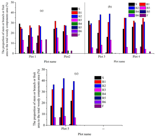
Figure 4. The proportion of stem, branch, and fruit area to the woody components area of each harvested tree in the five plots, respectively (S: stem, B1-B6: levels 1 to 6 branches, respectively, and F: fruit). (a): plots 1 and 2, (b): plots 3 and 4, (c): plot 5.

Table 3 shows that the proportions of the woody components area of those woody components with heights of <1.2 m to the woody components area of the harvested trees in each plot slightly vary amongst the five plots at a range of 2% to 6%. However, the proportions of the woody components area of the branches located below live canopies to the woody components area of the harvested trees in the five plots largely vary at a range of 1% to 21% (Table 3). The proportions of the woody components area of all branches located below live canopies to the woody components area of all harvested trees in each plot are the largest in plots 4 and 5 (0.18 and 0.21, respectively; Table 3) and smallest in plots 1 and 2 (0.01; Table 3).

Table 3. Proportions of the woody components area of those woody components with heights of <1.2 m (including stem and branches) or the branches located below live canopies to the woody components area of the harvested trees in each plot.

Proportions of the Woody Components Area of the Parts of the Woody Components to Woody Components Area of the Harvested Trees in Each Plot	Plot 1	Plot 2	Plot 3	Plot 4	Plot 5
Woody components with heights of <1.2 m	2%	2%	6%	4%	6%
All the branches located below live canopies	1%	1%	11%	18%	21%

Large variations can be observed amongst the $\alpha$ of the harvested trees in plots 3 to 5, especially plot 3 (Table 4). The variations in value and proportion of the $\alpha$ of harvested trees are 0.19 and 112% in plot 3 and <0.03 and 19% in plots 1 and 2 (Table 4). Large differences are also observed in the $\alpha$ of the five plots estimated with a measurement height of 0 m (Table 4). For example, the difference in proportion of the $\alpha$ in plots 1 and 5 reaches as large as 56% (Table 4). Compared with the $\alpha$ of plots 1 and 5, the difference in proportion of the $\alpha$ in plots 3 and 4 is relatively smaller and equivalent to 19% (the measurement height is 0 m). Meanwhile, only minor differences are observed between the $\alpha$ of plots 1 and 2 (2%; the measurement height is 0 m) (Table 4). The $\alpha$ of plots 4 and 5 are larger than those of the other three plots (Table 4). In sum, the variations in proportion of the $\alpha$ in the five plots estimated with two measurement heights of 0 m and 1.2 m range from 2% to 6% (Table 4). Hereinafter, only the plot $\alpha$ estimated using the destructive method with a measurement height of 1.2 m is regarded as the reference $\alpha$ of the five plots.

Table 4. The $\alpha$ of the harvested trees estimated via the destructive method with a measurement height of 0 m in each plot. The $\alpha$ of each plot was calculated by using Equation (15) with measurement heights of 0 m and 1.2 m.

Plot Name	Tree 1	Tree 2	Tree 3	Plot $\mathsf{\alpha }$
				Measurement Height: 0 m	Measurement Height: 1.2 m
Plot 1	0.16	0.16	0.17	0.16	0.16
Plot 2	0.16	0.19		0.17	0.16
Plot 3	0.22	0.17	0.36	0.21	0.20
Plot 4	0.27	0.21	0.28	0.25	0.24
Plot 5	0.19	0.25	0.28	0.25	0.23

4.2. ${\alpha }_e$ Estimates Obtained from DHP and MCI

Figure 5a shows that the proportions of the woody components pixel number to the classified leaf off period MCI image pixel number at zenith angles ranging from 0° to 80° with a 10° interval are remarkably larger than the proportions of the woody components pixel number to the classified leaf on MCI image pixel number at the same zenith angle in the five plots. For example, the proportions of the woody components pixel number to the classified leaf-on and leaf off periods MCI image pixel number in plot 1 are 0.15 and 0.62 at zenith angles 0° as well as 0.50 and 0.96 at zenith angles 80°, respectively (Figure 5a). For leaf-on forest canopies, the proportions of woody components shaded by shoots at zenith angles ranging from 0° to 80° with a 10° interval are large, especially at small zenith angles, and tend to decrease along with zenith angles in the five plots (Figure 5b). For example, the proportion of woody components shaded by shoots can reach as high as 0.70 at a 0° zenith angle, and decreases to 0.35 at a 80° zenith angle in plot 1 (Figure 5b). Meanwhile, the proportions of woody components shaded by shoots at a zenith angle ranging from 0° to 80° with a 10° interval are larger at those plots with fewer branches located below live canopies (plots 1 and 2) compared with those plots with a large number of branches (plots 4 and 5) (Figure 5b).

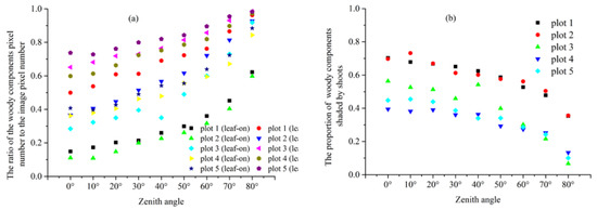
Figure 5. The proportion of the woody components pixel number to the classified MCI image pixel number (a) and the proportion of the woody components shaded by shoots, which is calculated by using the classified leaf-on and leaf-off periods MCI images (b) at zenith angles ranging from 0° to 80° with a 10° interval in the five plots. The proportion of the woody components shaded by shoots at each zenith angle is derived by taking the ratio of the shaded woody components pixels (calculated by subtracting the woody components pixel number of the classified leaf-on period MCI images from the woody components pixel number of the classified leaf-off period MCI images) to the total classified leaf-on period MCI image pixel number.

Table 5 shows that the ${\alpha }_e$ estimated by using the leaf-on and leaf-off periods DHP or MCI images is 2.29 to 4.63 times the reference $\alpha$ of the five plots regardless of the optical method and inversion model used in the ${\alpha }_e$ estimation. For example, the ${\alpha }_e$ derived using the leaf-on and leaf-off periods DHP images at plot 2 was ~4.63 times the reference $\alpha$ of plot 2 if the LAI-2200 inversion model was adopted in the ${\alpha }_e$ estimation (Table 4 and Table 5). Similarly, the ${\alpha }_e$ derived using the leaf-on and leaf-off periods MCI images at plot 2 was ~ 3.5 times the reference $\alpha$ of plot 2, if the MCI_0-85 inversion model was adopted in the ${\alpha }_e$ estimation (Table 4 and Table 5). The RMSE and MAE of the ${\alpha }_e$ derived using the leaf-on and leaf-off periods MCI or DHP images were larger than 0.41 (205%) and 0.40 (203%) in the five plots, respectively (Table 6). Similarly, the ${\alpha }_e$ derived from the percentage method by using the leaf-on period MCI images was 2.19 to 2.57 times the reference $\alpha$ of the five plots (Table 5). However, the ${\alpha }_e$ obtained by using the leaf-on period MCI images based on 57.3 and MCI_0-85 was closer to the reference $\alpha$ of the five plots whilst its RMSE and MAE were <0.05 (26%) and 0.04 (22%), respectively (Table 4, Table 5 and Table 6).

Table 5. ${\mathsf{\alpha }}_{\mathrm{e}}$ estimates obtained from DHP and MCI in the five plots.

Image Datasets	Leaf-on and Leaf-off Periods DHP Images			Leaf-on Period MCI Images			Leaf-on and Leaf-off Periods MCI Images
Inversion model	57.3	Miller	LAI-2200	57.3	MCI_0-85	Percentage	57.3	MCI_0-85
Plot 1	0.59	0.61	0.68	0.17	0.17	0.36	0.65	0.59
Plot 2	0.68	0.53	0.74	0.16	0.17	0.35	0.55	0.56
Plot 3	0.57	0.49	0.64	0.28	0.28	0.54	0.59	0.63
Plot 4	0.67	0.85	0.73	0.29	0.31	0.59	0.55	0.62
Plot 5	0.64	0.79	0.67	0.30	0.28	0.59	0.65	0.62

Table 6. Correlation statistics between the ${\alpha }_e$ estimated from DHP and MCI and the reference $\alpha$ of the five plots. Statistics are given at the 95% confidence level from the two-tailed Student’s t-test.

Image Datasets	Inversion Model	R2	Intercept	Slope	RMSE (in %)	MAE (in %)
Leaf-on and leaf-off periods DHP images	57.3	0.19	0.58	0.26	0.44 (221%)	0.43 (219%)
	Miller	0.78	0.01	3.23	0.47 (238%)	0.46 (231%)
	LAI-2200	−0.07	0.71	−0.08	0.50 (250%)	0.49 (249%)
Leaf-on period MCI images	57.3	0.95	−0.10	1.73	0.05 (26%)	0.04 (21%)
	MCI_0-85	0.956	−0.10	1.71	0.05 (26%)	0.04 (22%)
	Percentage	0.97	−0.14	3.16	0.30 (150%)	0.29 (145%)
Leaf-on and leaf-off periods MCI images	57.3	−0.03	0.61	−0.05	0.41 (205%)	0.40 (203%)
	MCI_0-85	0.82	0.47	0.66	0.41 (205%)	0.41 (205%)

Small differences (<7%) were observed between the ${\alpha }_e$ estimates obtained by using the leaf-on period MCI images based on 57.3 and MCI_0-85 in the five plots (Table 5). Similarly, the variations in proportion between the ${\alpha }_e$ estimates obtained using the leaf-on and leaf-off periods MCI images based on 57.3 and MCI_0-85 were <13% in the five plots (Table 5). By contrast, large differences were observed between the ${\alpha }_e$ estimates obtained by using the leaf-on and leaf-off periods DHP images based on 57.3 and Miller (3% to 27%), Miller and LAI-2200 (11% to 40%), and LAI-2200 and 57.3 (5% to 15%) in the five plots (Table 5).

4.3. $\alpha$ Estimates Obtained from DHP and MCI

The ${\alpha }_e$ estimates derived without consideration of ${\Omega }_e$ and ${\Omega }_w$ by using the leaf-on and leaf-off periods DHP or MCI images were systematically larger than those derived with consideration of ${\Omega }_e$ and ${\Omega }_w$ by using the same inversion model in the five plots (with the exception of the ${\alpha }_e$ estimates obtained by using the leaf-on and leaf-off periods DHP images based on the Miller inversion model in plots 2 and 3) (Table 4, Table 5, Table 7 and Table 8). Specifically, those $\alpha$ estimates obtained with consideration of ${\Omega }_e$ and ${\Omega }_w$ by using the leaf-on and leaf-off periods DHP or MCI images were 1.57 to 4.13 times larger than the reference $\alpha$ of the five plots (Table 4, Table 7 and Table 8). The RMSE and MAE of these $\alpha$ estimates derived using the leaf-on and leaf-off periods DHP or MCI images with consideration of ${\Omega }_e$ and ${\Omega }_w$ were >0.30 (153%) and 0.30 (150%) or 0.21 (107%) and 0.20 (103%) in the five plots, respectively, regardless of the ${\Omega }_e$ and ${\Omega }_w$ estimation algorithm and inversion model adopted in the estimation (Table 9 and Table 10).

Table 7. $\alpha$ estimates derived with consideration of ${\Omega }_e$ and ${\Omega }_w$ by using the leaf-on and leaf-off periods DHP images in the five plots.

Inversion Model	${\mathit{\Omega }}_{\mathit{e}}$ and ${\mathit{\Omega }}_{\mathit{w}}$ Estimation Algorithm	Plot 1	Plot 2	Plot 3	Plot 4	Plot 5
57.3	CC	0.45	0.57	0.49	0.57	0.47
	LX_5	0.41	0.57	0.50	0.53	0.46
	LX_15	0.41	0.59	0.50	0.55	0.47
	LX_30	0.44	0.60	0.51	0.55	0.47
	CLX_15	0.49	0.62	0.53	0.57	0.49
	CLX_30	0.47	0.62	0.50	0.57	0.46
	CLX_45	0.46	0.62	0.50	0.57	0.47
Miller	CC	0.50	0.49	0.45	0.72	0.59
	LX_5	0.51	0.54	0.51	0.69	0.56
	LX_15	0.51	0.52	0.51	0.71	0.58
	LX_30	0.52	0.51	0.50	0.72	0.59
	CLX_15	0.54	0.56	0.54	0.72	0.59
	CLX_30	0.53	0.55	0.52	0.72	0.58
	CLX_45	0.52	0.54	0.50	0.71	0.58
LAI_2200	CC	0.50	0.62	0.54	0.61	0.49
	LX_5	0.50	0.64	0.56	0.59	0.48
	LX_15	0.50	0.65	0.57	0.61	0.49
	LX_30	0.51	0.66	0.58	0.61	0.50
	CLX_15	0.54	0.66	0.59	0.62	0.52
	CLX_30	0.53	0.66	0.57	0.62	0.50
	CLX_45	0.52	0.66	0.56	0.61	0.50

Table 8. $\alpha$ estimates obtained with consideration of ${\Omega }_e$ and ${\Omega }_w$ by using the leaf-on period MCI images in the five plots.

Inversion Model	${\mathit{\Omega }}_{\mathit{e}}$ and ${\mathit{\Omega }}_{\mathit{w}}$ Estimation Algorithm	Leaf-on Period MCI Images					Leaf-on and Leaf-off Periods MCI Images
		Plot 1	Plot 2	Plot 3	Plot 4	Plot 5	Plot 1	Plot 2	Plot 3	Plot 4	Plot 5
57.3	CC	0.10	0.11	0.17	0.20	0.16	0.32	0.37	0.54	0.40	0.37
	LX	0.15	0.15	0.28	0.28	0.22	0.42	0.45	0.55	0.50	0.45
	CLX	0.16	0.16	0.31	0.31	0.26	0.44	0.47	0.57	0.55	0.48
MCI_0-85	CC	0.10	0.16	0.20	0.23	0.18	0.36	0.38	0.46	0.46	0.36
	LX	0.14	0.16	0.28	0.30	0.24	0.45	0.47	0.56	0.54	0.44
	CLX	0.15	0.17	0.30	0.33	0.28	0.47	0.48	0.60	0.57	0.48

Table 9. Correlation statistics between the obtained $\alpha$ (estimated with consideration of ${\Omega }_e$ and ${\Omega }_w$ by using the leaf-on and leaf-off periods DHP images) and the reference $\alpha$ of the five plots. Statistics are given at the 95% confidence level from the two-tailed Student’s t-test.

Inversion Model	${\mathit{\Omega }}_{\mathit{e}}$ and ${\mathit{\Omega }}_{\mathit{w}}$ Estimation Algorithm	R2	Intercept	Slope	RMSE (in %)	MAE (in %)
57.3	CC	0.15	0.47	0.22	0.32 (160%)	0.31 (158%)
	LX_5	0.10	0.46	0.17	0.30 (153%)	0.30 (150%)
	LX_15	0.08	0.48	0.15	0.31 (159%)	0.31 (155%)
	LX_30	−0.03	0.52	−0.05	0.32 (164%)	0.32 (160%)
	CLX_15	−0.16	0.59	−0.24	0.35 (176%)	0.34 (173%)
	CLX_30	−0.13	0.57	−0.25	0.33 (169%)	0.33 (165%)
	CLX_45	−0.12	0.57	−0.22	0.33 (169%)	0.33 (165%)
Miller	CC	0.76	0.13	2.12	0.36 (182%)	0.35 (179%)
	LX_5	0.73	0.28	1.43	0.37 (186%)	0.37 (185%)
	LX_15	0.79	0.21	1.81	0.37 (187%)	0.37 (185%)
	LX_30	0.81	0.18	1.98	0.37 (189%)	0.37 (187%)
	CLX_15	0.74	0.3	1.46	0.40 (200%)	0.40 (198%)
	CLX_30	0.7	0.28	1.49	0.38 (194%)	0.38 (192%)
	CLX_45	0.72	0.25	1.61	0.38 (190%)	0.37 (188%)
LAI_2200	CC	−0.03	0.56	−0.05	0.36 (183%)	0.36 (180%)
	LX_5	−0.19	0.62	−0.34	0.37 (184%)	0.36 (181%)
	LX_15	−0.14	0.61	−0.24	0.37 (188%)	0.36 (184%)
	LX_30	−0.14	0.62	−0.25	0.38 (191%)	0.37 (188%)
	CLX_15	−0.19	0.65	−0.30	0.39 (199%)	0.39 (196%)
	CLX_30	−0.22	0.65	−0.37	0.38 (194%)	0.38 (190%)
	CLX_45	−0.21	0.64	−0.37	0.38 (191%)	0.37 (187%)

Table 10. Correlation statistics between the obtained $\alpha$ estimates (derived with consideration of ${\Omega }_e$ and ${\Omega }_w$ by using the leaf-on period MCI images) and the reference $\alpha$ of the five plots. Statistics are given at the 95% confidence level from the two-tailed Student’s t-test.

Inversion Model	${\mathit{\Omega }}_{\mathit{e}}$ and ${\mathit{\Omega }}_{\mathit{w}}$ Estimation Algorithm	Leaf-on Period MCI Images					Leaf-on and Leaf-off Periods MCI Images
		R2	Intercept	Slope	RMSE (in %)	MAE (in %)	R2	Intercept	Slope	RMSE (in %)	MAE (in %)
57.3	CC	0.91	−0.06	1.03	0.05 (28%)	0.05 (27%)	0.27	0.28	0.59	0.22 (109%)	0.20 (103%)
	LX	0.84	−0.07	1.42	0.04 (19%)	0.03 (14%)	0.42	0.36	0.57	0.28 (141%)	0.28 (140%)
	CLX	0.86	−0.10	1.71	0.06 (31%)	0.04 (22%)	0.58	0.34	0.84	0.31 (155%)	0.31 (154%)
MCI_0-85	CC	0.82	−0.03	1.01	0.04 (18%)	0.03 (13%)	0.49	0.27	0.67	0.21 (107%)	0.21 (105%)
	LX	0.88	−0.10	1.64	0.04 (22%)	0.03 (16%)	0.34	0.39	0.49	0.30 (149%)	0.29 (147%)
	CLX	0.91	−0.14	1.96	0.06 (33%)	0.05 (26%)	0.45	0.38	0.70	0.33 (165%)	0.32 (163%)

Based on RMSE, MAE, and R², the accuracies of the $\alpha$ estimates derived using the leaf-on period MCI images with consideration of ${\Omega }_e$ and ${\Omega }_w$ showed little to no improvement compared with those estimates derived from the same inversion model but without consideration of ${\Omega }_e$ and ${\Omega }_w$ in the five plots (Table 6 and Table 10). The RMSE and MAE of the $\alpha$ estimated with consideration of ${\Omega }_e$ and ${\Omega }_w$ by using the leaf-on period MCI images were <33% and 27% in the five plots, respectively (Table 10).

For the DHP method, only slight differences (0% to 16%) were observed in the $\alpha$ estimated using the leaf-on and leaf-off periods DHP images based on the same inversion model but with different ${\Omega }_e$ and ${\Omega }_w$ estimation algorithms in the five plots (Table 7). No significant differences (0% to 22%) were also observed in the $\alpha$ estimated using the leaf-on and leaf-off periods DHP images based on the two inversion models of LAI-2200 and 57.3 but with the same ${\Omega }_e$ and ${\Omega }_w$ estimation algorithm in the five plots (Table 7). By contrast, large variations (0% to 30%) were observed in the $\alpha$ estimated using the leaf-on and leaf-off periods DHP images based on two groups of inversion models (Miller and 57.3 as well as Miller and LAI-2200) but with same ${\Omega }_e$ and ${\Omega }_w$ estimation algorithms in the five plots (Table 7).

For the MCI method, only small differences (2% to 18%) were observed in the $\alpha$ estimated using the leaf-on period or leaf-on and leaf-off periods MCI images based on the same inversion model but with different ${\Omega }_e$ and ${\Omega }_w$ estimation algorithms (except for CC) in the five plots (Table 8). However, large differences (0% to 82%) were observed in the $\alpha$ estimated using the leaf-on period or leaf-on and leaf-off periods MCI images based on the same inversion model but with different ${\Omega }_e$ and ${\Omega }_w$ estimation algorithms (include CC) in the five plots (Table 8). Meanwhile, only slight differences (0% to 9%) were observed in the $\alpha$ estimated using the leaf-on period or leaf-on and leaf-off periods MCI images based on the two inversion models with the same ${\Omega }_e$ and ${\Omega }_w$ estimation algorithms (excluding CC) in the five plots (Table 8). By contrast, obvious differences (0% to 45%) were observed in the $\alpha$ estimated using the leaf-on period or leaf-on and leaf-off MCI images based on the two inversion models with CC in the five plots (Table 8).

5. Discussion

5.1. Factors That Affect the Accuracy of the Reference $\alpha$ Estimates

The destructive method requires considerable time and effort to measure the reference $\alpha$ of forest plots. To reduce workload, some studies have simplified the measurement procedures, such as by discarding the fruits and parts of branches of the harvested trees [16]. For example, all branches (excluding B1, B2, and the end level branches) and fruits were not considered in estimating the reference $\alpha$ of forest plots in Chen [16]. However, the sum of the proportions of the B3, B4, and B5 branch areas and fruit areas to the total woody components area of the harvested trees ranges from 5% to 28% in the five plots (Figure 4). Therefore, simplifying the measurement procedures of the destructive method as can be seen in Chen [16] can introduce large bias in the reference $\alpha$ estimation of L. gmelinii forest plots. Such simplification cannot be directly used to measure the reference $\alpha$ of forest plots with different plant functional types. At least, this simplified method [16] is not accurate enough to estimate the reference $\alpha$ of L. gmelinii forest plots. However, based on the results in Figure 4, B4, B5, and B6 can all be neglected in estimating the reference $\alpha$ of L. gmelinii forest plots due to their small contributions to the woody components areas of the harvested trees in the five plots. By contrast, fruits should be considered in estimating the reference $\alpha$ because they are widely distributed across the forest canopies (Figure 4).

The mismatch between the measurement heights of the destructive and optical methods has usually been ignored in previous studies [16,23,33]. Specifically, these studies have estimated the reference $\alpha$ of forest plots with a measurement height of 0 m, but their optical instruments are usually operated and levelled above ground in the plots. Meanwhile, in this study, the DHP and MCI instruments were mounted on a tripod with a measurement height of about 1.2 m above ground. Therefore, the woody components and leaves or shoots of forest canopies with a height of < 1.2 m cannot be sampled by optical methods. Neglecting the mismatch in the measurement heights of harvesting and optical methods can introduce approximately 2% to 6% bias into the estimation of the woody components area and $\alpha$ of the harvested trees in the five plots (Table 3 and Table 4). Therefore, such mismatch must be considered when evaluating the performance of optical methods in estimating the $\alpha$ of forest plots.

5.2. Impact of Tree Age, Stand Density, Site Conditions, and Management Activities on the Reference $\alpha$ of Forest Plots

Management activities, such as removing the branches below live canopies are usually performed by forest managers to promote tree growth in forest plots. The proportion of the woody components area of all woody components located below live canopies to the woody components area of the harvested trees in plot 5 is 0.21 (Table 3), which indicates that management activities affect the reference $\alpha$ of forest plots obviously. If the woody components of the trees located below live canopies were not harvested for plots 1 and 2 during the thinning campaign prior the experiment and if the proportions of the woody components area of the woody components located below live canopies to the woody components area of the trees in plots 1, 2, and 5 were assumed to be the same, then the reference $\alpha$ of plots 1 and 2 would become equal to 0.19 and 0.19, respectively. The variations in proportion between the recalculated $\alpha$ of plots 1 and 2 and the reference $\alpha$ of plot 5 were approximately 21%. Given that no obvious differences can be found in the site conditions of the three plots, the variations between the recalculated $\alpha$ of plots 1 and 2 and the reference $\alpha$ of plot 5 were mainly attributed to tree age and stand density. On the other hand, the large variations in the reference $\alpha$ of plots 1, 2, and 5 also be indicative of the larger role of management activities (relative to tree age or stand density) in increasing the large difference in the reference $\alpha$ of the five plots.

Plots 3 and 4 sharing similar characteristics, including tree age, mean tree height, and average DBH (Table 2). Furthermore, those branches with a height of ~ ≤ 2.5 m were low- and medium-level harvested in plots 3 and 4 prior the experiment, respectively. Plot 4 had poorer site conditions compared with plot 3 because this plot had many yellow needles distributed amongst its canopies and had a larger dry soil depth as compared with plot 3. However, the reference $\alpha$ of plot 4 was 20% larger than that of plot 3 thereby indicating that site conditions affect the reference $\alpha$ of forest plots obviously (Table 4).

In conclusion, tree age, stand density, site conditions, and management activities contribute to the large differences in the reference $\alpha$ of the five selected L. gmelinii plots (Table 2 and Table 4). Therefore, these four factors must be considered when estimating the reference $\alpha$ of L. gmelinii plots. Amongst these factors, site conditions and management activities have the largest contributions to the variations in the reference $\alpha$ of the L. gmelinii plots. Meanwhile, the reference $\alpha$ of those forest plots with the same tree species and similar characteristics of stand density and tree age yet with different levels of branch removal and site conditions must be dissimilar. A specific $\alpha$ estimate should be obtained for those forest plots (Table 2, Table 3 and Table 4). The same can be said for those forest plots with the same tree species, branch removal levels and site conditions yet with different stand density and tree age (Table 2, Table 3 and Table 4). However, those forest plots with the same tree species and similar characteristics of stand density, site conditions, tree age, and management activities (e.g., plots 1 and 2) must show slight variations in their reference $\alpha$ (Table 2 and Table 4). Chen [16] also reported small differences (13%) in the reference $\alpha$ of two Picea mariana plots with similar stand density, tree age, tree height, and management activities. This argument is consistent with the findings of this study.

5.3. Factors That Affect the $\alpha$ Estimation of the Two Optical Methods

Figure 5 and Table 5, Table 6, Table 7, Table 8, Table 9 and Table 10 reveal that the performance of DHP and MCI in estimating the $\alpha$ of forest plots is influenced by four factors, namely, the inversion model, the clumping effects of canopy element and woody components, the ${\Omega }_e$ and ${\Omega }_w$ estimation algorithms, and the preferential shading of woody components by shoots. Amongst these factors, the inversion model only slightly influences the ${\alpha }_e$ or $\alpha$ estimation of forest plots, if 57.3, LAI-2200 and MCI_0-85 are used in the estimation (Table 5, Table 7 and Table 8). Meanwhile, the ${\alpha }_e$ or $\alpha$ estimates obtained using the leaf-on and leaf-off periods DHP images based on Miller and 57.3 as well as Miller and LAI-2200 showed relatively larger differences compared with those estimated by 57.3 and LAI-2200. This finding is consistent with the conclusions of Zou et al. [15], who reported small differences (<10%) in the ${\mathrm{WAI}}_{\mathrm{e}}$, ${\mathrm{PAI}}_{\mathrm{e}}$, $\mathrm{WAI}$, and PAI of leaf-on and leaf-off forest canopies estimated using LAI-2200 and 57.3. Relatively large differences (2% to 17%) were also observed in the $WA{I}_e$, $PA{I}_e$, $\mathrm{WAI}$, and PAI that were estimated using Miller and 57.3 as well as Miller and LAI-2200 [15]. Such variations can be attributed to the fact that the gap fraction measurements collected from DHP at zenith angles near the horizon tend to approach zero. When using Miller in estimating PAI and WAI, the null gap fraction measurements could introduce errors into the estimations even if the null gap fraction measurements processing solutions were applied [15]. Zou et al. [15] pointed out that several inversion models, including LAI-2200 and 57.3, can avoid such effect. Given that accurate $\alpha$ estimates were obtained by using leaf-on period MCI images based on MCI_0-85 (similar to LAI-2200) and 57.3 in the five plots (Table 8 and Table 10), both 57.3 and MCI_0-85 suggest to be used in the $\mathsf{\alpha }$ estimation of forest plots.

The ${\alpha }_e$ or $\alpha$ estimates obtained with or without consideration of ${\Omega }_e$ and ${\Omega }_w$ using the leaf-on and leaf-off periods DHP or MCI images were 1.57 to 4.63 times the reference $\alpha$ of the five plots (Table 4, Table 5, Table 7 and Table 8). Given that the $WA{I}_e$ and WAI of leaf-on forest plots were derived by using leaf-off period DHP or MCI images, the overestimation of ${\alpha }_e$ and $\alpha$ indicates that the $PA{I}_e$ and PAI of leaf-on forest plots are significantly underestimated when leaf-on period DHP or MCI images are used in the $PA{I}_e$ and PAI estimation. Moreover, the underestimation of the $PA{I}_e$ and PAI of leaf-on forest plots was mainly driven by the underestimation of $WA{I}_e$ and WAI because of the obvious differences in the proportions of woody components pixel number to the leaf-on and leaf-off periods MCI image pixel numbers at the zenith angles ranging from 0° to 80° with a 10° interval in the five plots (Figure 5a). The underestimation of the ${\mathrm{WAI}}_{\mathrm{e}}$ and WAI of leaf-on forest plots can also be reflected in the large proportions of woody components shaded by shoots at zenith angles ranging from 0° to 80° with a 10° interval (Figure 5b). The shading of woody components by shoots in canopies increases the woody components gap fraction of forest canopies as their WAI should be, thereby resulting in the underestimation of ${\mathrm{WAI}}_{\mathrm{e}}$ and WAI. However, the overestimation of ${\alpha }_e$ or $\alpha$ can be largely reduced if only the leaf-on period MCI images are used in the ${\alpha }_e$ or $\alpha$ estimation (Table 4, Table 5 and Table 8) because the underestimation of the denominator (${\mathrm{PAI}}_{\mathrm{e}}$ or PAI) and numerator (${\mathrm{WAI}}_{\mathrm{e}}$ or WAI) cancels out the ${\alpha }_e$ or $\alpha$ estimation errors to a large degree. The underestimation of the $WA{I}_e$ and WAI of leaf-on period forest plots as estimated using leaf-on period MCI or DHP images reveals the obvious overestimation of ${\alpha }_e$ and $\alpha$ in the five plots, which were obtained using leaf-on and leaf-off periods DHP or MCI images, can be attributed to the fact that the woody components are preferentially shaded by shoots. In L. gmelinii forest canopies, the shoots are directly located on the branch and stem surfaces, thereby leading to preferential shading of branches and stems.

The woody components of forest canopies include stems, branches, and fruits. Given that these woody components are not randomly distributed in space similar to leaves or shoots, both the clumping effects of the canopy element and woody components should be considered in estimating the $\alpha$ of forest plots. However, minor differences were observed between the RMSE and MAE of the ${\alpha }_e$ and $\alpha$ estimates obtained using the leaf-on period MCI images without or with consideration of ${\Omega }_e$ and ${\Omega }_w$ (Table 6 and Table 10). Therefore, the clumping effects of the canopy element and woody components of leaf-on forest canopies are not effectively evaluated by the adopted ${\Omega }_e$ and ${\Omega }_w$ estimation algorithms regardless of the ${\Omega }_e$ and ${\Omega }_w$ estimation algorithm and segment size used in the ${\alpha }_e$ and $\alpha$ estimation. Previous studies have also reported that the ${\Omega }_e$ and ${\Omega }_w$ estimation algorithms used in this study do not always perform well in estimating the ${\Omega }_e$ and ${\Omega }_w$ of all leaf-on and leaf-off forest canopies with different plant functional types, tree species composition, PAI, and WAI [15,27,46]. For example, Zou et al. [15] observed small differences between the majority of the WAI estimates derived using 57.3 or LAI-2200 with consideration of ${\Omega }_w$ (derived from CC, LX, and CLX) and the WAI of leaf-off birch forest plots. However, large differences were observed between the majority of the PAI estimates (derived by using the same inversion model and ${\mathsf{\Omega }}_{\mathrm{e}}$ estimation algorithm) and the PAI of leaf-on birch forest plots [15]. This report indicates that the ${\Omega }_w$ of leaf-off birch forest plots was effectively estimated by using the three ${\Omega }_e$ and ${\Omega }_w$ estimation algorithms; by contrast, the ${\Omega }_e$ of leaf-on birch forest plots was not effectively estimated by using these algorithms [15]. Accurately estimating $\alpha$ depends on both accurate PAI and WAI estimates whilst accurately estimating PAI and WAI estimates, in turn, relies on both accurate estimates of ${\Omega }_e$ and ${\Omega }_w$. Therefore, the mismatch between the performance of ${\Omega }_e$ and ${\Omega }_w$ estimation algorithm in estimating the ${\Omega }_e$ and ${\Omega }_w$ of leaf-on and leaf-off forest plots can introduce errors into the estimation of $\alpha$. The fact of the preferential shading of woody components by shoots can also influence the performance of ${\Omega }_e$ and ${\Omega }_w$ estimation algorithms in evaluating the clumping effects of the canopy element and woody components of leaf-on forest canopies.

5.4. Determining Whether Accurate $\alpha$ Estimates Can Be Obtained from DHP and MCI

Table 4, Table 5, Table 6, Table 7, Table 8, Table 9 and Table 10 reveal that relatively accurate $\alpha$ estimates with estimation errors of lower than 20% can be obtained from MCI in the L. gmelinii plots. If no errors are exist in the LAI estimation of L. gmelinii forest plots except in estimating $\alpha$, then MCI can be considered an effective method that meets the required maximum LAI estimation error (20%) for in situ LAI estimates specified by GCOS. Unlike DHP, MCI can discriminate leaves or shoots, woody components and sky based on the NIR and VIS band images of forest canopies. DHP has the disadvantage of the insufficient sampling of forest canopies at zenith angles close to the zenith due to the intrinsic defect of hemispherical photography. The proportions of woody components shaded by shoots at zenith angels ranging from 0° to 85° with a 10° interval are large at those zenith angles close to the zenith in the five plots (Figure 5b). Therefore, for DHP, the estimation errors in the $p_e\left(\theta \right)$, $p_w\left(\theta \right)$, ${\Omega }_e\left(\theta \right)$, and ${\Omega }_w\left(\theta \right)$ measurements with zenith angles close to zenith can introduce bias into the $\alpha$ estimation of forest plots. By contrast, MCI can obtain images with sufficient sampling of forest canopies at all directions of the upper hemisphere and is thereby recommended for estimating the $\alpha$ of forest plots.

The methods adopted in previous studies [17,18,19,20] for estimating the $\alpha$ of forest plots by using leaf-on and leaf-off periods DHP images or radiation attenuation measurements can introduce significant errors into the estimations (Table 4, Table 5, Table 6, Table 7, Table 8, Table 9 and Table 10). Therefore, these methods would not suggested to be used in estimating the $\alpha$ of forest plots, at least for L. gmelinii forest plots. The percentage method also overestimated the $\mathsf{\alpha }$ in the five plots (Table 5), thereby indicating that this method must not be used in estimating the $\alpha$ of L. gmelinii forest sites. This conclusion contradicts the report of Woodgate [13], who found a 3% difference in the $\mathsf{\alpha }$ estimated by the percentage method and the reference $\alpha$ of eucalypt forest scenes. The contrasting canopy structures of the tree species covered in Woodgate and in this study may explain such contradiction.

5.5. Limitations and Perspectives

Given the huge amount of time and effort required by the destructive method to measure the $\alpha$ of forest sites, only two or three representative trees were harvested for each plot in this study. Considering the obvious variations between the $\alpha$ of the harvested trees in each plot (Table 4), more representative trees must be harvested to obtain highly reliable and accurate estimations of the reference $\alpha$ of forest plots. For example, three trees can be harvested for each class of dominant, codominant, and suppressed trees in each plot. Given that only five plots were covered in this study, the impact of tree age or stand density on estimating the reference $\alpha$ of forest plots was not evaluated. More forest plots (>5) must be covered in the future to obtain highly reliable conclusions regarding the influence of tree age, stand density, site conditions and management activities on estimating the reference $\alpha$ of L. gmelinii forest plots. More plant functional types must also be covered in the future to check whether MCI can effectively measure the $\alpha$ of forest sites with different tree species compositions.

6. Conclusions

The conclusions of this study are as follows. (1) The woody components area of harvested trees mainly comprises of the woody components areas of branches and fruits. Caution is needed when parts of woody components, especially fruits, are discarded in estimating the $\mathsf{\alpha }$ of harvested trees. The mismatch in the measurement heights of destructive and optical methods should also be considered in the $\alpha$ estimation of forest plots. (2) Large variations (0% to 56%) are observed in the reference $\alpha$ of the five plots with the same tree species yet with different tree age, stand density, site conditions, and management activities. Moreover, the impact of site conditions and management activities on the reference $\alpha$ of forest plots is larger than that of tree age and stand density. (3) The performance of DHP and MCI in estimating the $\alpha$ of forest plots is obviously affected by the inversion model and the preferential shading of woody components by shoots in leaf-on canopies. The large overestimation of the $\alpha$ (i.e., 1.57 to 4.63 times larger than the reference value for this study) that was derived using leaf-on and leaf-off periods DHP or MCI images can be mainly attributed to the preferential shading of woody components by leaves or shoots. The impact of the adopted ${\Omega }_e$ and ${\Omega }_w$ estimation algorithms on estimating the $\alpha$ of forest plots is relatively small. (4) Relatively accurate $\alpha$ estimates (with estimation errors of <20%) can be obtained from MCI if the appropriate inversion model and ${\Omega }_e$ and ${\Omega }_w$ estimation algorithm are used in the $\alpha$ estimation of L. gmelinii forest plots.

References

- Fernandes, R.; Plummer, S.; Nightingale, J.; Baret, F.; Camacho, F.; Fang, H.; Garrigues, S.; Gobron, N.; Lang, M.; Lacaze, R.; et al. Global Leaf Area Index Product Validation Good Practices (Version 2.0). In Best Practice for Satellite-Derived Land Product Validation (p. 76): Land Product Validation Subgroup (WGCV/CEOS); Gabriela, S.-S., Miguel, R., Eds.; NOAA, USGS, NASA, College Park: USA, 2014. [Google Scholar]
- Watson, D.J. Comparative physiological studies in the growth of field crops. I. Variation in net assimilation rate and leaf area between species and varieties, and within and between years. Ann. Bot. 1947, 11, 41–76. [Google Scholar] [CrossRef]
- Chen, J.M.; Black, T.A. Defining leaf area index for non-flat leaves. Plant. Cell. Environ. 1992, 15, 421–429. [Google Scholar] [CrossRef]
- Baret, F.; Hagolle, O.; Geiger, B.; Bicheron, P.; Miras, B.; Huc, M.; Berthelot, B.; Niño, F.; Weiss, M.; Samain, O.; et al. Lai, fapar and fcover cyclopes global products derived from vegetation: Part 1: Principles of the algorithm. Remote Sens. Environ. 2007, 110, 275–286. [Google Scholar] [CrossRef]
- Feng, D.; Chen, J.M.; Plummer, S.; Mingzhen, C.; Pisek, J. Algorithm for global leaf area index retrieval using satellite imagery. IEEE Trans. Geosci. Remote Sens. 2006, 44, 2219–2229. [Google Scholar] [CrossRef]
- Xiao, Z.; Liang, S.; Wang, J.; Chen, P.; Yin, X.; Zhang, L.; Song, J. Use of general regression neural networks for generating the glass leaf area index product from time-series modis surface reflectance. IEEE Trans. Geosci. Remote Sens. 2014, 52, 209–223. [Google Scholar] [CrossRef]
- Knyazikhin, Y.; Martonchik, J.V.; Myneni, R.B.; Diner, D.J.; Running, S.W. Synergistic algorithm for estimating vegetation canopy leaf area index and fraction of absorbed photosynthetically active radiation from modis and misr data. J. Geophys. Res. Atmos. 1998, 103, 32257–32275. [Google Scholar] [CrossRef]
- Baret, F.; Weiss, M.; Lacaze, R.; Camacho, F.; Makhmara, H.; Pacholcyzk, P.; Smets, B. Geov1: Lai and fapar essential climate variables and fcover global time series capitalizing over existing products. Part1: Principles of development and production. Remote Sens. Environ. 2013, 137, 299–309. [Google Scholar] [CrossRef]
- Fang, H.; Jiang, C.; Li, W.; Wei, S.; Baret, F.; Chen, J.M.; Garcia-Haro, J.; Liang, S.; Liu, R.; Myneni, R.B.; et al. Characterization and intercomparison of global moderate resolution leaf area index (lai) products: Analysis of climatologies and theoretical uncertainties. J. Geophys. Res. Biogeosci. 2013, 118, 529–548. [Google Scholar] [CrossRef]
- Garrigues, S.; Lacaze, R.; Baret, F.; Morisette, J.T.; Weiss, M.; Nickeson, J.E.; Fernandes, R.; Plummer, S.; Shabanov, N.V.; Myneni, R.B.; et al. Validation and intercomparison of global leaf area index products derived from remote sensing data. J. Geophys. Res. Biogeosci. 2008, 113. [Google Scholar] [CrossRef]
- Jingming, C. Remote sensing of leaf area index of vegetation covers. In Remote Sensing of Natural Resources; Weng, Q., Ed.; CRC Press: Boca Raton, FL, USA, 2014; p. 24. [Google Scholar]
- Yan, K.; Park, T.; Yan, G.; Liu, Z.; Yang, B.; Chen, C.; Nemani, R.; Knyazikhin, Y.; Myneni, R. Evaluation of modis lai/fpar product collection 6. Part 2: Validation and intercomparison. Remote Sens. 2016, 8, 460. [Google Scholar] [CrossRef]
- Woodgate, W. In-Situ Leaf Area Index Estimate Uncertainty in Forests: Supporting Earth Observation Product Calibration and Validation. Ph.D. Thesis, RMIT University, Melbourne, Australia, 2015. [Google Scholar]
- Zou, J.; Yan, G.; Zhu, L.; Zhang, W. Woody-to-total area ratio determination with a multispectral canopy imager. Tree Physiol. 2009, 29, 1069–1080. [Google Scholar] [CrossRef] [PubMed]
- Zou, J.; Zhuang, Y.; Chianucci, F.; Mai, C.; Lin, W.; Leng, P.; Luo, S.; Yan, B. Comparison of seven inversion models for estimating plant and woody area indices of leaf-on and leaf-off forest canopy using explicit 3d forest scenes. Remote Sens. 2018, 10, 1297. [Google Scholar] [CrossRef]
- Chen, J.M. Optically-based methods for measuring seasonal variation of leaf area index in boreal conifer stands. Agric. For. Meteorol. 1996, 80, 135–163. [Google Scholar] [CrossRef]
- Barclay, H.J.; Trofymow, J.A.; Leach, R.I. Assessing bias from boles in calculating leaf area index in immature douglas-fir with the li-cor canopy analyzer. Agric. For. Meteorol. 2000, 100, 255–260. [Google Scholar] [CrossRef]
- Bréda, N.J.J. Ground-based measurements of leaf area index: A review of methods, instruments and current controversies. J. Exp. Bot. 2003, 54, 2403–2417. [Google Scholar] [CrossRef] [PubMed]
- Liu, Z.; Wang, C.; Chen, J.M.; Wang, X.; Jin, G. Empirical models for tracing seasonal changes in leaf area index in deciduous broadleaf forests by digital hemispherical photography. For. Ecol. Manag. 2015, 351, 67–77. [Google Scholar] [CrossRef]
- Toda, M.; Richardson, A.D. Estimation of plant area index and phenological transition dates from digital repeat photography and radiometric approaches in a hardwood forest in the northeastern united states. Agric. For. Meteorol. 2018, 249, 457–466. [Google Scholar] [CrossRef]
- Kucharik, C.J.; Norman, J.M.; Murdock, L.M.; Gower, S.T. Characterizing canopy nonrandomness with a multiband vegetation imager (mvi). J. Geophys. Res. Atmos. 1997, 102, 29455–29473. [Google Scholar] [CrossRef]
- Sea, W.B.; Choler, P.; Beringer, J.; Weinmann, R.A.; Hutley, L.B.; Leuning, R. Documenting improvement in leaf area index estimates from modis using hemispherical photos for australian savannas. Agric. For. Meteorol. 2011, 151, 1453–1461. [Google Scholar] [CrossRef]
- Gower, S.T.; Kucharik, C.J.; Norman, J.M. Direct and indirect estimation of leaf area index, fapar, and net primary production of terrestrial ecosystems. Remote Sens. Environ. 1999, 70, 29–51. [Google Scholar] [CrossRef]
- Deblonde, G.; Penner, M.; Royer, A. Measuring leaf area index with the li-cor lai-2000 in pine stands. Ecology 1994, 75, 1507–1511. [Google Scholar] [CrossRef]
- Chen, J.M.; Govind, A.; Sonnentag, O.; Zhang, Y.; Barr, A.; Amiro, B. Leaf area index measurements at fluxnet-canada forest sites. Agric. For. Meteorol. 2006, 140, 257–268. [Google Scholar] [CrossRef]
- Nilson, T. A theoretical analysis of the frequency of gaps in plant stands. Agric. Meteorol. 1971, 8, 25–38. [Google Scholar] [CrossRef]
- Leblanc, S.G.; Fournier, R.A. Hemispherical photography simulations with an architectural model to assess retrieval of leaf area index. Agric. For. Meteorol. 2014, 194, 64–76. [Google Scholar] [CrossRef]
- Weiss, M.; Baret, F.; Smith, G.J.; Jonckheere, I.; Coppin, P. Review of methods for in situ leaf area index (lai) determination: Part II. Estimation of lai, errors and sampling. Agric. For. Meteorol. 2004, 121, 37–53. [Google Scholar] [CrossRef]
- Baret, F.; de Solan, B.; Lopez-Lozano, R.; Ma, K.; Weiss, M. Gai estimates of row crops from downward looking digital photos taken perpendicular to rows at 57.5° zenith angle: Theoretical considerations based on 3d architecture models and application to wheat crops. Agric. For. Meteorol. 2010, 150, 1393–1401. [Google Scholar] [CrossRef]
- Liu, Z.; Jin, G.; Chen, J.; Qi, Y. Evaluating optical measurements of leaf area index against litter collection in a mixed broadleaved-korean pine forest in china. Trees 2015, 29, 59–73. [Google Scholar] [CrossRef]
- Miller, J. A formula for average foliage density. Aust. J. Bot. 1967, 15, 141–144. [Google Scholar] [CrossRef]
- LI-COR. Lai-2200 Plant Canopy Analyzer Instruction Manual; LI-COR Cor.: Lincoln, NE, USA, 2009. [Google Scholar]
- Chen, J.M.; Rich, P.M.; Gower, S.T.; Norman, J.M.; Plummer, S. Leaf area index of boreal forests: Theory, techniques and measurements. J. Geophys. Res. 1997, 102, 29429–29444. [Google Scholar] [CrossRef]
- Lang, A.R.G.; Yueqin, X. Estimation of leaf area index from transmission of direct sunlight in discontinuous canopies. Agric. For. Meteorol. 1986, 37, 229–243. [Google Scholar] [CrossRef]
- Gonsamo, A.; Pellikka, P. The computation of foliage clumping index using hemispherical photography. Agric. For. Meteorol. 2009, 149, 1781–1787. [Google Scholar] [CrossRef]
- Chen, J.M.; Cihlar, J. Plant canopy gap-size analysis theory for improving optical measurements of leaf-area index. Appl. Opt. 1995, 34, 6211–6222. [Google Scholar] [CrossRef] [PubMed]
- Chen, J.M.; Cihlar, J. Quantifying the effect of canopy architecture on optical measurements of leaf area index using two gap size analysis methods. IEEE Trans. Geosci. Remote Sens. 1995, 33, 777–787. [Google Scholar] [CrossRef]
- Pisek, J.; Lang, M.; Nilson, T.; Korhonen, L.; Karu, H. Comparison of methods for measuring gap size distribution and canopy nonrandomness at järvselja rami (radiation transfer model intercomparison) test sites. Agric. For. Meteorol. 2011, 151, 365–377. [Google Scholar] [CrossRef]
- Leblanc, S.G.; Chen, J.M.; Fernandes, R.; Deering, D.W.; Conley, A. Methodology comparison for canopy structure parameters extraction from digital hemispherical photography in boreal forests. Agric. For. Meteorol. 2005, 129, 187–207. [Google Scholar] [CrossRef]
- Walter, J.-M.N.; Fournier, R.A.; Soudani, K.; Meyer, E. Integrating clumping effects in forest canopy structure: An assessment through hemispherical photographs. Can. J. Remote Sens. 2003, 29, 388–410. [Google Scholar] [CrossRef]
- Zou, J.; Yan, G.; Chen, L. Estimation of canopy and woody components clumping indices at three mature picea crassifolia forest stands. Sel. Top. Appl. Earth Observ. Remote Sens. IEEE J. 2015, 8, 1413–1422. [Google Scholar] [CrossRef]
- Liu, Z.; Jin, G.; Qi, Y. Estimate of leaf area index in an old-growth mixed broadleaved-korean pine forest in northeastern china. PLoS ONE 2012, 7, e32155. [Google Scholar]
- Gower, S.T.; Vogel, J.G.; Norman, J.M.; Kucharik, C.J.; Steele, S.J.; Stow, T.K. Carbon distribution and aboveground net primary production in aspen, jack pine, and black spruce stands in saskatchewan and Manitoba, Canada. J. Geophys. Res. Atmos. 1997, 102, 29029–29041. [Google Scholar] [CrossRef]
- Leblanc, S.G.; Chen, J.M. Tracing Radiation and Architecture of Canopies Trac Manual Version 2.1.3; Natural Resources Canada: Ottawa, ON, Canada, 2002; p. 25. [Google Scholar]
- Gonsamo, A.; Pellikka, P. Methodology comparison for slope correction in canopy leaf area index estimation using hemispherical photography. For. Ecol. Manag. 2008, 256, 749–759. [Google Scholar] [CrossRef]
- Macfarlane, C.; Grigg, A.; Evangelista, C. Estimating forest leaf area using cover and fullframe fisheye photography: Thinking inside the circle. Agric. For. Meteorol. 2007, 146, 1–12. [Google Scholar] [CrossRef]
© 2018 by the authors. Licensee MDPI, Basel, Switzerland. This article is an open access article distributed under the terms and conditions of the Creative Commons Attribution (CC BY) license (http://creativecommons.org/licenses/by/4.0/).