Development of a PM_2.5 Emission Factor Prediction Model for Shrubs in the Xiao Xing’an Mountains Based on Coupling Effects of Physical Factors

Abstract

Over recent years, the intensity of forest fires has escalated, with wildfire-emitted pollutants exerting substantial impacts on the environment, ecosystems, and human well-being. This study developed a robust predictive framework to quantify wildfire-induced PM_2.5 emission factors (EFs) using seven shrub species—Corylus mandshurica, Eleutherococcus senticosus, Philadelphus schrenkii, Sorbaria sorbifolia, Syringa reticulata, Spiraea salicifolia, and Lonicera maackii. These species represent ecological cornerstones of Northeast Asian forests and hold global relevance as widely introduced or invasive taxa in North America and Europe. The novelty of this research lies in the integration of traditional statistical inference with machine learning to resolve the complex coupling between fuel traits and emissions. We conducted 1134 laboratory-controlled burns in the Liangshui National Nature Reserve, evaluating two continuous and three categorical variables. Initial screening via Analysis of Variance (ANOVA) and stepwise linear regression (Step-AIC) identified the primary drivers of emissions and revealed that interspecific differences among the seven shrubs did not significantly affect the EF (p = 0.0635). To ensure statistical rigor, a log-transformation was applied to the EF data to correct for right-skewness and heteroscedasticity inherent in raw observations. Linear Mixed-effects Models (LMMs) and Gradient Boosting Machines (GBMs) were subsequently employed to quantify factor effects and capture potential nonlinearities. The LMM results consistently identified burning type and plant part as the dominant determinants: smoldering combustion and leaf components exerted strong positive effects on PM_2.5 emissions compared to flaming and branch components. Fuel load was positively correlated with emissions, while moisture content showed a significant negative effect. Notably, the model identified a significant negative quadratic effect for moisture content, indicating a non-linear inhibitory trend as moisture increases. While interspecific differences among the seven shrubs did not significantly affect EFs suggesting that physical fuel traits exert a more consistent influence than species-specific genetic backgrounds, complex interactions were captured. These include a negative synergistic effect between leaves and smoldering, and a positive interaction between moisture content and leaves that significantly amplified emissions. This research bridges the gap between physical fuel traits and chemical smoke production, providing a high-resolution tool for refining global biomass burning emission inventories and assisting international forest management in similar temperate biomes.

1. Introduction

Fire plays a pivotal role in forest ecosystems: by clearing dead branches and leaves it improves soil aeration and water circulation, while also promoting the succession of particular species and supporting ecosystem renewal and recovery. To maintain natural reproduction and succession with minimal structural damage, prescribed fire is commonly employed. Compared with wildfires, prescribed fire yields significantly lower carbon emissions [1] and can reduce the likelihood of crown fires for at least five years after burning [2]. It also achieves additional objectives such as facilitating the regeneration of specific plant species or serving as an effective tool for restoring grasslands on encroached land [3,4]. Overall, fire is one of the primary drivers shaping ecosystem structure and function, broadly influencing nutrient cycling, vegetation structure and composition, and the distribution of herbivores [5].

Conversely, forest fires can contribute to climate change [6], and the impacts of climate change have, in turn, markedly increased the frequency and intensity of forest fires in recent years [7,8]. Wildfires damage trees and cause substantial soil carbon losses [9], disrupt ecosystem balance, and can even permanently alter forest landscapes and structure. During wildfires, biomass combustion significantly elevates ambient concentrations of aerosol pollutants in affected regions [10]; in some areas, PM_2.5 from wildfires has supplanted mobile and industrial sources as the dominant contributor [11,12]. Once ignited, smoke particles travel far and affect wide areas [13]; for many events the emission source lies outside the affected jurisdiction, with surface concentration increases originating hundreds to thousands of kilometers away [14]. The atmospheric impacts of PM_2.5 ultimately bear on human health and survival: although data do not show that sharp, short-term PM_2.5 increases directly raise daily mortality [15], PM_2.5 is closely linked to the aggravation of health problems [16] and is associated with cardiovascular mortality, emergency room visits, and annual non-accidental mortality [17]. PM_2.5 can also contribute to central nervous system disorders, including neurodegenerative diseases such as Alzheimer’s disease [18]. There is even evidence that wildfire-derived PM_2.5 poses a greater health threat [19]. Economically, smoke impacts may be at least comparable to the direct costs of the fires themselves [20].

Forest fires are broadly categorized—based on the ignition source, propagation velocity, impacted area, and severity—into surface, crown, and underground fires. Surface fires are most common, accounting for more than 90% of forest fires [21]. The surface biotic layer is a major forest component, comprising nearly 40% of total biomass in some forests [22], and surface plants can be almost completely consumed during fires [23]. Surface fires therefore have considerable pollution potential. Their principal fuels include understory shrubs and grasses as well as dead branches and leaves on the forest floor; studies show that the fuels contributing the greatest mass to emissions are predominantly shrubs and duff [24]. In a survey conducted in Northeast China, the significance of dominant shrubs within the shrub category surpasses that of the primary herbaceous plants within the herbaceous category [25]. Meanwhile, the biomass of individual shrub plants is also higher than that of herbaceous plants. In the surface fires with the highest probability of occurrence, shrubs have a high biomass and low richness, while also having a high importance value, making their contribution to the fire very noteworthy. However, significant research gaps remain in characterizing smoke emissions from understory vegetation. Most existing studies focus on arborescent or herbaceous species, leaving the specific contributions of shrubs—the most susceptible and dominant component of the surface biotic layer—largely under-quantified. Furthermore, although individual variables like moisture content (MC) and fuel load (FL) are known to affect emissions, few studies have explicitly defined the complex interaction effects and non-linear coupling between these factors.

Each forested area warrants a distinct examination. Influenced by climate, site conditions, species composition, and human activities, spatial and temporal heterogeneity in species distribution and biomass is pronounced among regions. In Heilongjiang Province, China—within a temperate humid zone under a continental monsoon climate—even a single forest can show substantial variation in shrub and herb types and distributions across broad leaf, coniferous, and mixed conifer–broad leaf forests. In recent years, indoor ignition simulations have been widely used to analyze fire behavior [26,27], while remote sensing has been applied to assess the quantity and composition of smoke from landscape fires [28,29]. Quantifying forest-fire emissions is challenging because their spatio-temporal patterns differ markedly from anthropogenic sources [30,31,32]. Consequently, some researchers have integrated remote sensing techniques with controlled indoor burning experiments to evaluate the environmental impact of forest fire pollutants and derive combustion emission factors [33]. In this study, we conducted a series of controlled indoor burning experiments on the primary shrub species in Liangshui National Nature Reserve using filter membrane sampling and weighing techniques. We manipulated various experimental variables and quantitatively determined PM_2.5 emissions from different biomass components under various combustion types. The research explored the effects of variables such as moisture content and fuel load on biomass combustion smoke during forest fires, as well as the contributions of different plant part to PM_2.5 emissions. The objective was to furnish foundational data and scientific evidence concerning the impact of forest fire smoke emissions on forest ecosystems and the broader environment.

The novelty of this research lies in its integrated approach to resolving these gaps by bridging traditional statistical inference with machine learning. Specifically, we address the statistical limitations inherent in raw emission factor (EF) data, such as heteroscedasticity, by applying log-transformations to ensure robust Linear Mixed-effects Model (LMM) performance. By quantifying the non-linear quadratic effects of moisture and the synergistic interactions between plant parts and combustion modes, this study provides a high-resolution predictive framework. Our primary objective is to furnish foundational data for seven ecologically dominant shrub species that possess both regional importance in Northeast Asia and global relevance as widespread or invasive taxa in North America and Europe. This ensures that our scientific evidence concerning PM_2.5 emissions serves as a versatile tool for forest ecosystem management and air quality assessment across similar temperate biomes globally.

To bridge the identified knowledge gaps, this study was designed to address the following fundamental questions:

Can a unified predictive model accurately quantify PM_2.5 emissions across diverse shrub species, or does interspecific variation necessitate species-specific emission factors?

To what extent do physical fuel properties (moisture content and load) and biological components (leaves vs. branches) interact with combustion modes to determine the total particulate output?

Is the relationship between moisture content and smoke emission strictly linear, or do complex non-linear thresholds and synergistic interactions exist that significantly alter emission profiles?

2. Materials and Methods

2.1. Study Area Description

The Liangshui Experimental Forest Farm of Northeast Forestry University, also known as the Liangshui National Nature Reserve, was established in 1958. Situated on the eastern slope of the Dali Dailing branch in the southern section of the Xiao Xing’an Mountains in northeastern China, it spans a total area of 12,133 hm². Its geographical coordinates range from 128°47′8″ E to 128°57′19″ E and 47°6′49″ N to 47°16′10″ N. Geographically, the reserve lies on the eastern edge of the Eurasian continent and is significantly influenced by a marine climate, exhibiting distinct characteristics of a temperate continental monsoon climate. The area features both pristine forests that have never been harvested and secondary forests that have undergone burning or clearing, representing various stages of forest succession. Additionally, it includes artificial forests of red pine, spruce, larch, and camphor pine, as well as mixed forests of various types. This reserve serves as a true microcosm of the Xiao Xing’an Mountains prior to its development, offering valuable insights into the original “baseline” conditions of the Xiao Xing’an Mountains forest ecosystem (Figure 1).

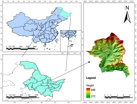
Figure 1. Schematic diagram of remote sensing information of the Liangshui area.

The vegetation in the reserve is classified into six main types: northern coniferous forest, temperate mixed forest, deciduous broad-leaved forest, shrubs, grasslands, and wetlands, supporting rich biodiversity. The fauna includes numerous species of amphibians, reptiles, birds, mammals, insects, and fungi. This region is also a critical ecological habitat for endangered species, such as Astragalus koraiensis and Taxus cuspidata. Dominant shrub species include Corylus heterophylla, Spiraea salicifolia, Eleutherococcus senticosus, and Syringa reticulata, which together account for over 89% of the area’s importance.

In contrast, dominant herbaceous species are composed of various plants, including Deyeuxia angustifolia, Arex dispalata, Filipendula palmata, Maianthemum bifolium, Carex callitrichos and Equisetum sylvaticum, etc. The cumulative importance value of these dominant herbaceous species exceeds 28% within the herbaceous layer [34]. The Liangshui National Nature Reserve prioritizes the protection of its ecological environment and biodiversity, implementing a series of measures to mitigate the impact of human activities on the ecosystem. These measures include prohibiting hunting, restricting tourism development, and promoting environmental education. Unlike the forest fires frequently observed in the Great Xing’an mountains area, Liangshui has established more effective fire prevention measures, resulting in no recorded fires over the past 71 years. However, this prolonged absence of fire has disrupted nutrient cycling, reduced soil fertility, and led to the accumulation of significant fuel loads, creating a substantial fire hazard. Although there has been no targeted or detailed investigation into the distribution of shrub vegetation within the Liangshui area, relevant research indicates that the understory vegetation biomass in forests of northern China—including the Great Xing’an mountains, Xiao Xing’an Mountains, and Changbai Mountains—accounts for approximately 6.2% of the total forest biomass, with validated average of 6.59 t/hm² [35] and 2.5 t/hm² [36].

2.2. Sampling and Pretreatment

We conducted indoor combustion analysis experiments on common tree species in Liangshui to evaluate the potential for PM_2.5 release under varying moisture content conditions, specifically focusing on species prevalent in the Great Xing’an mountains region. However, comprehensive combustion data related to shrubs are notably lacking in the existing literature. In designing our experiments, we considered the multitude of factors influencing forest fires, encompassing seasonality, temperature, humidity, precipitation, wind speed and direction, stand age, canopy coverage, elevation, and slope aspect [37,38]. In this study, seven representative shrub species were selected from the Liangshui National Nature Reserve. These included Corylus mandshurica (CMM), Spiraea salicifolia (SSL), Eleutherococcus senticosus (ES), Sorbaria sorbifolia (SS), and Syringa reticulata (SR). Additionally, two other common shrubs in Northeast China, Lonicera chrysantha (LC) and Philadelphus schrenkii (PR), were included to ensure comprehensive regional representation. These species are subsequently referred to by their respective abbreviations throughout the text. Shrubs occupy the lower strata of the forest and are less affected by wind speed. Unlike particles produced by crown fires, particles generated by shrub combustion experience more favorable conditions for condensation and growth [39]. Therefore, wind speed was not selected as a variable in this experiment. Humidity and precipitation affect moisture content, while PM_2.5 release factors are positively correlated with load and moisture content [40]. Based on the sampling conditions and a comprehensive consideration of fire hazards, we focused on two components of the summer sampling (leaves and branches) to augment our understanding of PM_2.5 emissions during forest-fire combustion. The experiment employed three fuel-load levels (1 g, 2 g, 3 g) and five moisture content levels (10%, 15%, 20%, 25%, 40%). At 40% moisture content, only smoldering combustion was tested, whereas the other groups underwent comparative experiments between flaming and smoldering, with each group repeated three times.

Due to significant distribution differences among shrub species, we collected leaves and branches from multiple individuals across several shrub groups, including CMM, SSL, ES, SS, SR, LC, and PR. For each species, samples were taken from various heights, positions, and aspects on the sample plants. Depending on species size, 20–40 individuals per species were sampled, yielding approximately 2000 g of branches and leaves. After sampling, branches were cut into 2–3 cm segments and, within each species and organ, manually homogenized to ensure uniformity. The homogenized samples were then sealed in plastic bags to prevent moisture loss, and their weights were recorded.

Pretreatment involved air-drying and oven-drying, including determinations of moisture content, air-dried moisture content, and recovered moisture content.

Upon the arrival of the collected shrub samples at the laboratory, they were meticulously recombined and subsequently segregated into two sets for each type. The weight of each portion was recorded, and different symbols were marked for identification. One set was positioned in a cool, arid indoor environment to undergo natural air-drying for approximately thirty days, following which the weight of the air-dried samples was ascertained. The other portion was dried in an oven at 105 °C until constant weight was achieved (defined as a change in moisture content of <0.1% measured every 3 h). The dry weight—representing the absolute oven-dry weight—was measured using an electronic balance with 0.01 g precision. After drying, samples were sealed and stored. Owing to limited oven capacity, any undried samples were stored in a cool, dry area of the laboratory to prevent mold and deterioration that could otherwise affect subsequent experiments.

The moisture content (P) of different organs was calculated using the following formula, and organ-specific biomass was converted based on moisture content. By summing the biomass of different organs, biomass per unit area was determined. The formulas for calculating shrub-layer biomass and moisture content are as follows:

$${\mathrm{M}\mathrm{C}}_{\mathrm{a}}={\displaystyle \frac{{\mathrm{m}}_{\mathrm{a}}-{\mathrm{m}}_{\mathrm{d}}}{{\mathrm{m}}_{\mathrm{d}}}}\times 100\%$$

(1)

$${\mathrm{M}\mathrm{C}}_{\mathrm{o}}={\displaystyle \frac{{\mathrm{m}}_{\mathrm{o}}-{\mathrm{m}}_{\mathrm{d}}}{{\mathrm{m}}_{\mathrm{d}}}}\times 100\%$$

(2)

In the formula, ${\mathrm{M}\mathrm{C}}_{\mathrm{a}}$ represents the air-drying moisture content of the fuel, ${\mathrm{M}\mathrm{C}}_{\mathrm{o}}$ represents the oven-drying moisture content of the fuel, ${\mathrm{m}}_{\mathrm{a}}$ represents the air-dry weight of the fuel, ${\mathrm{m}}_{\mathrm{o}}$ represents the oven-dry weight of the fuel, and ${\mathrm{m}}_{\mathrm{d}}$ represents the original weight of the fuel (unit: kilograms).

2.3. Experiments

Upon completion of the sampling and preprocessing phases, each specimen provided three distinct mass measurements: the initial mass, the mass after air-drying, and the absolute dry mass. Subsequent analysis then quantified two additional metrics for the processed material—the recovered moisture content and the air-dried moisture content.

This study focuses on PM_2.5 emissions during biomass combustion in forest fires. To examine the effects of key variables on PM_2.5 release, ensure appropriate instrument detection limits and combustion efficiency, and simulate realistic smoldering and open-burning conditions, we conducted preliminary experiments. Based on these trials, we selected fuel loads of 1 g, 2 g, and 3 g, and moisture contents of 10%, 15%, 20%, and 25% for seven shrub species, including both branches and leaves. Each fuel load was paired with all moisture content levels, and separate experiments were designed for flaming and smoldering, with each condition repeated three times. For the 14 distinct samples, the total number of experimental combinations was: 3 (fuel-load levels) × 4 (moisture content levels) × 3 (repetitions) × 2 (combustion types) = 72 test units per sample. To determine whether samples approached the upper limit of PM_2.5 release capacity, we added three further sets at 40% moisture with fuel loads of 1 g, 2 g, and 3 g for each sample. Because preliminary tests showed most 40%-moisture samples could not sustain positive combustion, only smoldering experiments were performed. In total, 1134 data points were collected. Across samples, recovered moisture content varied markedly and air-dried moisture content also differed; overall, the air-dried moisture content consistently ranged between 30% and 45%.

The experimental apparatus comprised a combustion bed, a particulate-matter sampler, and a PM_2.5 concentration monitor. All simulated burns were conducted inside a fume hood at the laboratory of Northeast Forestry University.

Across all trials, a standardized lighter served as the ignition source. To reproduce burning types observed in natural wildfires, biomass placed on a wire-mesh combustion bed was heated with an alcohol lamp. An asbestos mesh was overlaid on the bed to (i) minimize heat loss, (ii) promote uniform heat distribution, and (iii) isolate open flames as much as possible. The bed was kept horizontally, and its dimensions were adjusted to accommodate the volumes of branches and leaves associated with different fuel loads.

This experiment quantified PM_2.5 by filter-membrane sampling with gravimetric determination: a glass-fiber filter (pore size ≈ 0.3 μm) intercepted airborne particles with ~99.99% efficiency, and PM_2.5 mass was computed from the pre-/post-sampling filter-weight difference. PM_2.5 was collected using a medium-flow environmental sampler (JCH-6120F; Qingdao Juchuang, Qingdao, China) at 100 L·min⁻¹; the pump maintained a constant flow, an upstream size-cut removed particles > 2.5 μm, and the remaining aerosol then passed through the in-line glass-fiber filter. The sampling duration was synchronized to readings from a laboratory PM_2.5 monitor (GQ-058; Shenzhen Jishun An Technology Co., Ltd., Shenzhen, China), which employs an infrared source and light-scattering detection, where the scattered-light intensity, proportional to particle concentration, is converted to electrical signals and displayed after processing. During pre-tests of the combustion setup, we recorded the time required for indoor PM_2.5 to return to baseline; to standardize collection and ensure complete capture within the enclosure, subsequent trials used a fixed sampling time of 17 min. The experimental setup is illustrated in Figure 2.

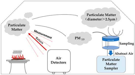
Figure 2. Diagram of combustion chamber and experimental equipment.

The experimental procedure was conducted as follows:

Prior to the commencement of experiments, a pristine, planar glass-fiber filter was examined for the presence of pinholes and subsequently affixed within a numbered holder. Subsequently, the filters underwent conditioning within a controlled-environment chamber set at a temperature of 25 °C and a relative humidity of 50% for a duration of 24 h. Following this, they were weighed using an electronic balance (FA2004N; Shanghai Sunny Hengping Scientific Instrument Co., Ltd., Shanghai, China); precision of 0.0001 g). The sampler inlet was then opened, and the filter was meticulously smoothed out using tweezers and positioned securely before the sampler was reassembled. Prior to the initiation of formal experimental runs, a blank control was established by operating the system in the absence of fuel combustion and subsequently recording the PM_2.5 levels from the chamber.

To prepare samples and adjust moisture, small sealed bags were first weighed and opened. Each one was filled with 10 g of sample; twenty bags were prepared per sample and divided into four groups. Water was sprayed onto each group as required, bags were sealed, and all were conditioned for ≥12 h prior to testing.

For combustion, the pre-weighed sample was spread evenly on the combustion bed. The particulate sampler was switched on, an alcohol lamp was ignited with a standard igniter, and the cabinet door was promptly closed. Two ignition protocols were used: for smoldering, only the alcohol lamp was lit; for open-flame combustion, vapors/smoke released after heating were rapidly ignited.

After each trial, the filter was removed with tweezers and the upstream size-cut blade was cleaned with anhydrous ethanol to avoid contamination of subsequent collections. The loaded filter was re-equilibrated in the same chamber (25 °C, 50% relative humidity) to minimize moisture effects on PM_2.5 mass, and its post-sampling weight was measured and recorded.

In this study, emission factors (EF) were used to evaluate pollutant emissions. An EF represents the mass of pollutants released per unit mass of fuel burned or per unit energy produced. The PM_2.5 EF for each combustion experiment was calculated using the following formula:

$${\mathrm{E}\mathrm{F}}_{{\mathrm{P}\mathrm{M}}_{2.5}}={\displaystyle \frac{{\mathrm{m}}_{\mathrm{P}\mathrm{M}}}{{\mathrm{m}}_{\mathrm{b}\mathrm{u}\mathrm{r}\mathrm{n}\mathrm{e}\mathrm{d}}}}$$

(3)

where

${\mathrm{E}\mathrm{F}}_{{\mathrm{P}\mathrm{M}}_{2.5}}$: emission factor for PM_2.5 (g⋅kg⁻¹);

${\mathrm{m}}_{\mathrm{P}\mathrm{M}}$: mass of PM_2.5 (g);

${\mathrm{m}}_{\mathrm{b}\mathrm{u}\mathrm{r}\mathrm{n}\mathrm{e}\mathrm{d}}$: mass of fuel burned (kg).

To ensure the reliability of the emission factor (EF) measurements, we performed a comprehensive uncertainty analysis. The experimental error primarily stems from three sources: mass weighing, flow rate regulation, and analytical replication.

First, fuel and filter masses were measured using a high-precision electronic balance (±0.01 mg uncertainty). Second, the sampling flow rate was maintained by a mass flow controller with a stability of ±2%. According to the error propagation law, the cumulative uncertainty of the calculated PM_2.5 EF was estimated to be less than 5.4%. This margin of error is significantly lower than the observed statistical differences between experimental groups, confirming that the identified trends in emission factors are driven by fuel traits rather than measurement noise.

2.3.1. ANOVA Table

We first used analysis of variance (ANOVA) in R (version 4.5.1) to screen main effects and low-order interactions. ANOVA partitions the total variation into components attributable to predefined sources and reports, for each source, the degrees of freedom (df), sum of squares, mean square (MS), F statistic and the associated p-value to test whether factor levels differ in their mean response.

Univariate (one-way) ANOVAs were run for moisture content (MC), fuel load (FL), plant part (PP), species (Spec) and burning type (BT). Guided by these results and data exploration, we then fit two-way ANOVAs for MC × FL and BT × PP to probe key interactions. Because the response structure suggested possible higher-order interplay, an exploratory three-way ANOVA was additionally conducted for FL × MC × PP (stratified by BT).

2.3.2. StepAIC

Given the clear factor structure and the need for interpretability, we fitted a multiple linear regression with the EF (PM_2.5 emission factor) as the response and FL, MC, PP and BT as predictors, considering all main effects and pairwise interactions.

EF ~ FL × MC × PP × Spec × BT

(4)

Bidirectional stepwise selection based on Akaike’s Information Criterion (AIC) was implemented with stepAIC (MASS), starting from the main-effects model and allowing terms up to the two-way boundary above. This selection process was primarily employed to achieve model parsimony and to provide a formal statistical validation of significant interactions. Recognizing the potential instability and bias inherent in stepwise AIC, we did not rely on it as the sole selection criterion; instead, it was used to refine a candidate model space pre-defined by biological relevance. To mitigate selection risks, we cross-validated the resulting structure and variable importance rankings against a Gradient Boosting Machine (GBM) to ensure consistency across parametric and non-parametric benchmarks.

2.3.3. Linear Mixed-Effects Model (LMM)

To ensure the robustness of our statistical inferences, a log-transformation was applied to the emission factor (EF) data as a primary preprocessing step. This procedure was necessitated by two critical considerations: first, the raw EF observations exhibited inherent right-skewness and heteroscedasticity, and the transformation ensured the data adhered more closely to the assumptions of residual normality and homoscedasticity required for LMM; second, the log-linear structure effectively captured the non-linear response relationships between EFs and the diverse set of explanatory variables. Notably, preliminary sensitivity analyses via StepAIC confirmed that the importance ranking of primary factors remained consistent regardless of whether the transformation was applied, further validating the reliability of this approach.

To address the issue of non-independence among observations pertaining to the same species, a linear mixed-effects model incorporating a species-specific random intercept was employed. The continuous predictor variables were subjected to centering and scaling procedures, resulting in z-scores. Additionally, a quadratic term for MC was incorporated based on data-driven considerations. The final fixed-effects structure was determined through a stepwise screening process, which retained only the most significant interactions.

Models were estimated with REML (lme4/lmerTest). We report coefficient estimates (and multiplicative effects on the original scale via exp(β)), marginal/conditional R² and the intraclass correlation coefficient (ICC).

2.3.4. Gradient Boosting Machine (GBM)

As a predictive benchmark that can capture nonlinearities and implicit higher-order interactions without manual specification, we trained a gradient boosting machine (GBM, Gaussian loss). Hyperparameters were set a priori (learning rate 0.01, maximum depth 4, subsampling 0.8, minimum observations per leaf 5), and the number of trees was chosen by 5-fold cross-validation with early stopping on the training folds. Categorical variables (PP, BT) were treated as factors; we did not engineer interaction terms. Performance was summarized with out-of-fold RMSE, MAE and R², and relative influence scores were used to rank predictor importance.

All models used the same 5-fold split for fair comparison; in addition, leave-one-species-out (LOSO) validation was performed for the LMM to assess across-species generalization. Analyses were conducted in R.

3. Results

3.1. Patterns and Determinants of PM_2.5 Emission Factors

3.1.1. Data Analysis

Based on the data analyzed from the ANOVA table, we identified that fuel load (FL), moisture content (MC), and plant part serve as significant predictors of the emission factor. While ‘burning type’ (BT) was evaluated, it primarily demonstrated influence through its interactions with other factors rather than as a standalone main effect. Interactions exist between ‘fuel load and moisture content’, ‘moisture content and plant part’, and ‘plant part and combustion method’. However, there is insufficient evidence to indicate interactions between ‘fuel load and plant part’, or among ‘fuel load, plant part, and moisture content’. This table provides valuable guidance for the subsequent design and optimization of figures. ANOVA results for the significance of main and interaction effects of the experimental variables are presented in Table 1.

Table 1. Results of the ANOVA on categorized experimental variables.

Source	DF	Sum Sq.	Mean Sq.	F Value	p
Species	6	465	77.57	1.997	0.0635
FL	2	3042	4521.2	53.991	<0.01
MC	3	4490	1496.6	53.115	<0.01
PP	1	809	809	31.254	<0.01
BT	1	46	46	1.763	0.185
FL:MC	6	1286	214.3	7.607	<0.01
FL:PP	2	155	77.6	2.753	0.0643
FL:BT	2	1792	896.0	26.040	<0.01
MC:BT	3	379	126.5	3.673	0.0119
MC:PP	3	1666	555.3	19.708	<0.01
PP:BT	1	12,502	12,502	482.911	<0.01
FL:MC:PP	6	176	29.3	1.038	0.3987

Although no interaction was observed between plant parts and fuel load, significant interactions were identified between plant parts and other variables. Consequently, we systematically differentiated the plant parts across various species and generated multiple visual representations.

3.1.2. Data Visualization

We differentiated plant parts across species and assembled a compact visualization suite capturing species-level EF distributions, load/moisture response trends, multivariate heatmaps, load–moisture interactions, and part-wise comparisons under different combustion modes.

The image summarizes PM_2.5 emission factors for seven shrub species—CMM, ES, LC, PR, SR, SS, and SSL—pooling observations from different plant parts under two combustion modes and multiple loading levels; measurements at 40% moisture content were excluded. In each box, the interquartile range (IQR) spans the middle 50% of observations from the first to the third quartile (Q1–Q3); the internal horizontal line marks the median, and whiskers extend to the dataset’s minimum and maximum values as plotted.

LC displays the widest IQR, indicating greater dispersion, whereas PR shows the narrowest IQR, reflecting more consistent values (see Figure 3). Among the species, SR exhibits the highest median emission factor, while ES exhibits the lowest. These patterns point to some interspecific contrasts and motivate further inquiry into their causes. Nonetheless, the extensive overlap among boxplots—together with the p-value of 0.0635—suggests that species differences do not significantly affect the emission factors.

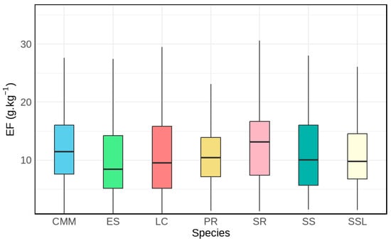
Figure 3. Boxplot Distribution Characteristics of PM_2.5 Emission Factors for Seven Shrub Species.

For a more intuitive visualization of emission factors across plant components, we constructed a two-dimensional heatmap (Figure 4). Rows encode fuel-load levels, with every three consecutive rows grouped to represent a single species. Columns encode moisture content, with every four adjacent columns grouped to indicate plant parts. The color scale maps PM_2.5 emission factors—lighter shades denote lower values, darker shades higher values. For clarity, we collectively refer to all panels pertaining to a given species and plant part as a “set of graphs.”

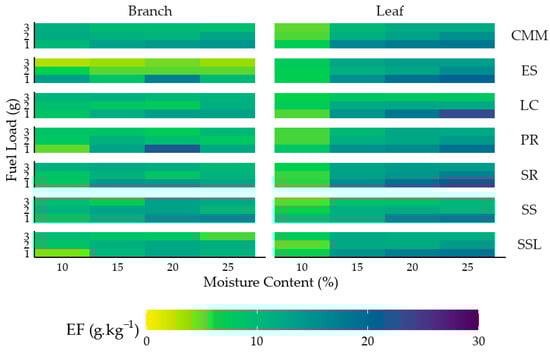
Figure 4. Two-Dimensional heatmaps of two plant components from seven shrub species under different moisture contents and fuel loads.

Across all branch panels, color intensity increases along the top-left to bottom-right diagonal, indicating a positive association between moisture content and emission factors and a negative association between fuel load and emission factors within each panel. Moreover, dominant hues are highly similar across species, suggesting minimal species effects on emission factors. Leaf heatmaps exhibit analogous patterns to the branch panels, with overall color intensities that are comparable or nearly identical.

3.2. Multiple Linear/Nonlinear Regression Fitting

3.2.1. StepAIC-Optimized Linear Regression

After fitting the two-way interaction model, the starting AIC was 2741.3 (Table 2). Backward stepwise evaluation showed that dropping any single interaction increased AIC (e.g., FL × Part: 2749.2; MC × BT: 2762.2; FL × MC: 2801.8; MC × Part: 2833.4; FL × BT: 2847.1; Part × BT: 3350.5), so the AIC-guided procedure retained the full two-way specification:

Table 2. Comparison of regression models before and after StepAIC optimization.

	Sum of Sq.	RSS	AIC
<none>	-	14,965	2771.3
FL:Part	148.2	15,112	2749.2
MC:BT	345.1	15,309	2762.2
FL:MC	957.7	15,922	2801.8
MC:Part	1465.0	16,429	2833.4
FL:BT	1689.7	16,554	2847.1
Part:BT	124,476.4	27,440	3350.5

Rules of thumb for AIC differences are: ΔAIC < 2 indicates substantial support, 4–7 indicates considerably less support, and ΔAIC > 10 indicates essentially no support. In our analysis, the best model has AIC = 2741.26. Dropping any single two-way interaction increased AIC—FL × Part: 2749.2 (ΔAIC ≈ 7.9), MC × BT: 2762.2 (ΔAIC ≈ 21.0), FL × MC: 2801.8 (ΔAIC ≈ 60.5), MC × Part: 2833.4 (ΔAIC ≈ 92.1), FL × BT: 2847.1 (ΔAIC ≈ 105.8), and Part × BT: 3350.5 (ΔAIC ≈ 609.2). Thus, all reduced models are considerably less supported or unsupported by the AIC. The stepwise procedure therefore retained the full two-way specification, and there is no evidence that removing interactions improves fit or parsimony.

$$\begin{gathered} \mathrm{E}\mathrm{F}={\beta }_0+{\beta }_1\mathrm{F}\mathrm{L}+{\beta }_2\mathrm{M}\mathrm{C}+{\beta }_3\mathrm{L}\mathrm{e}\mathrm{a}\mathrm{f}+{\beta }_4\mathrm{S}\mathrm{m}\mathrm{o}\mathrm{l}\mathrm{d}\mathrm{e}\mathrm{r}\mathrm{i}\mathrm{n}\mathrm{g}+{\beta }_5\left(\mathrm{F}\mathrm{L}\cdot \mathrm{M}\mathrm{C}\right)+{\beta }_6\left(\mathrm{F}\mathrm{L}\cdot \mathrm{L}\mathrm{e}\mathrm{a}\mathrm{f}\right)+{\beta }_7\left(\mathrm{F}\mathrm{L}\cdot \mathrm{S}\mathrm{m}\mathrm{o}\mathrm{l}\mathrm{d}\mathrm{e}\mathrm{r}\mathrm{i}\mathrm{n}\mathrm{g}\right) \\ +{\beta }_8\left(\mathrm{M}\mathrm{C}\cdot \mathrm{L}\mathrm{e}\mathrm{a}\mathrm{f}\right)+{\beta }_9\left(\mathrm{M}\mathrm{C}\cdot \mathrm{S}\mathrm{m}\mathrm{o}\mathrm{l}\mathrm{d}\mathrm{e}\mathrm{r}\mathrm{i}\mathrm{n}\mathrm{g}\right)+{\beta }_{10}\left(\mathrm{L}\mathrm{e}\mathrm{a}\mathrm{f}\cdot \mathrm{S}\mathrm{m}\mathrm{o}\mathrm{l}\mathrm{d}\mathrm{e}\mathrm{r}\mathrm{i}\mathrm{n}\mathrm{g}\right)+\mathsf{\epsilon } \end{gathered}$$

(5)

where:

$$\mathsf{\epsilon }\sim \mathrm{N}(0,3.8742)$$

(6)

Table 3 reports the estimated regression coefficients and associated p-values for all main effects and two-way interaction terms. The intercept represents the baseline condition (branch under flaming) at the reference moisture and load values.

Table 3. AIC-constrained stepwise regression (stepAIC): retained terms and model fit (response = EF).

Term	Estimate (βx)	p-Value
Intercept (β0)	1.218	0.342
FL (β1)	0.604	0.259
MC (β2)	0.659	<0.001
Part = Leaf (β3)	3.165	0.002
BT = Smoldering (β4)	4.776	<0.001
FL × MC (β5)	−0.214	<0.01
FL × Leaf (β6)	−0.939	0.002
FL × Smoldering (β7)	+3.171	<0.001
MC × Leaf (β8)	+0.431	<0.001
MC × Smoldering (β9)	−0.209	<0.001
Leaf × Smoldering (β10)	−14.073	<0.001

Among the main effects, moisture content (MC) and burning type (BT) show strong positive associations with the emission factor (both p < 0.001), while fuel load (FL) is not significant by itself. Compared with branches, leaves yield a significantly higher emission factor (β = 3.165, p = 0.002).

Several interaction terms are statistically significant, indicating that the effect of each predictor depends on the levels of the others. For example, the negative FL × MC term shows that the combined influence of load and moisture is less than additive—higher load weakens the moisture-driven increase in emissions. The large negative Leaf × Smoldering coefficient (β = −14.073, p < 0.001) further implies that leaf emissions under smoldering are substantially lower relative to the reference condition.

Overall, both main effects and interactions play important roles, confirming that fuel load, moisture content, plant part and burning type do not act independently on PM_2.5 emissions.

3.2.2. Performance of Linear Mixed-Effects Models’

To account for non-independence among observations from the same species, we fit a linear mixed-effects model with a species-level random intercept. Continuous predictors were centered and scaled (z-scores) and a data-driven quadratic term for MC was included. The final fixed-effects structure was determined through stepwise screening, retaining the strongest interactions and resulting in the following model (Table 4).

Table 4. LMM fixed effects on log(EF) with 95% CIs and multiplicative effects.

Term	β (log)	95% CI (log)	exp (β)	95% CI	p Value
Intercept	−4.6860	[−4.772, −4.600]	0.00923	[0.008, 0.010]	<0.001
zFL	+0.2493	[0.2180, 0.2806]	1.283	[1.244, 1.324]	<0.001
zMC	−0.1556	[−0.2075, −0.1037]	0.856	[0.813, 0.902]	5.39 × 10−9
zMC2	−0.09783	[−0.1247, −0.0710]	0.907	[0.883, 0.932]	1.64 × 10−12
Part (Leaf)	+1.2570	[1.161, 1.353]	3.515	[3.194, 3.867]	<0.001
BT (Smoldering)	+0.8447	[0.752, 0.938]	2.327	[2.121, 2.554]	<0.001
Leaf × Smoldering	−1.3860	[−1.517, −1.256]	0.250	[0.220, 0.285]	<0.001
zMC × Leaf	+0.8170	[0.752, 0.882]	2.264	[2.122, 2.415]	<0.001

To provide a rigorous statistical basis beyond descriptive observations, the optimal fixed-effects structure was first determined through a bidirectional stepwise screening process guided by Akaike’s Information Criterion (Step-AIC). This procedure allowed for a formal statistical validation of complex interactions, retaining only the most significant terms to ensure model parsimony. Based on the robust statistical support provided by the Step-AIC results and the subsequent LMM coefficients, we then constructed targeted visualizations to further elucidate these significant interaction effects and non-linear trends.

After identifying load as a significant determinant of the emission factor in our LMM analysis (β = 0.2493), we plotted load–PM_2.5 EF curves for each species (Figure 5) in our LMM analysis (β = 0.2493). Branches and leaves were analyzed separately using the same dataset described earlier. Observations from different plant parts across two combustion types and multiple load levels were included, while measurements at 40% moisture content were excluded. For each group, the mean of three replicate measurements was used. Unless otherwise specified, these data underpin the analyses that follow.

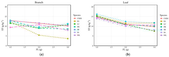
Figure 5. Line Graphs of PM_2.5 Emission Factors for Two Plant Tissues of Seven Shrub Species as a Function of Loading Capacity: (a) PM_2.5 emission factors for branches; (b) PM_2.5 emission factors for leaves).

In the branch plots, EFs generally decreased with increasing load, although curve shapes differed among species—likely reflecting variation in branch structure, morphology, or composition. Except for CMM, most species displayed smoother, predominantly broken-line rends, with SSL and PR even showing reversals. In contrast to the less predictable branch patterns, the leaf curves were more consistently downward across species. This aligns with the LMM’s identification of “Part (Leaf)” as a dominant factor with the highest positive effect size (β = 1.2570); LC exhibited an almost linear decline, whereas for the other species the slopes flattened as load increased.

In the moisture–EF curves (Figure 6), the overall pattern exhibits a clear upward trajectory, which seemingly contrasts with the LMM’s negative primary slope for moisture β= −0.1556). This observed increase, particularly in the leaf samples (Figure 6b), underscores the LMM’s conclusion that plant organs significantly influence the emission factor. Although the branch data appear more scattered, the presence of the significant negative quadratic term (zMC², β= −0.09783) in the LMM confirms a non-linear sensitivity; this suggests that at these moderate moisture levels, the dominant influence of the combustion mechanism effectively constrains the initial inhibitory effect of water. For leaves, this upward trend is further amplified by the robust positive zMC × Leaf interaction (β = 0.8170), causing leaf EFs to progressively diverge and exceed branch EFs as moisture increases.

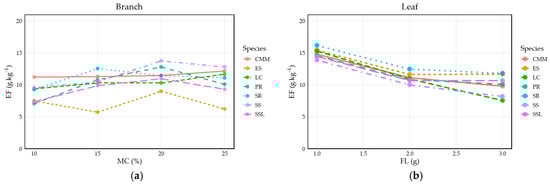
Figure 6. Line graphs of PM_2.5 emission factors for two plant tissues of seven shrub species as a function of moisture content: (a) PM_2.5 emission factors for branches; (b) PM_2.5 emission factors for leaves).

Figure 7 depicts the response of the PM_2.5 release factor to two drivers—fuel load and moisture content. Consistent with the LMM results identifying load as a significant positive determinant (β = 0.2493), Figure 7 demonstrates that loading exerts a pronounced effect on emissions, while its magnitude is further modulated across moisture levels. Interaction analysis confirms that these two variables do not act independently; their joint effect involves complex synergies where PM_2.5 responses become exceptionally sensitive at lower loading and lower moisture levels. This empirical pattern provides visual evidence for the LMM’s capacity to capture non-linear factor combinations, clarifying how specific fuel traits interact to alter the overall emission profile.

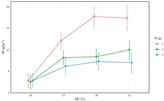
Figure 7. Line Charts of Impact Factor Variation with Moisture Content under Different Fuel Load Levels.

A comparative analysis of the emission profiles reveals that while branch curves generally lie above leaf curves within smoldering panels, this vertical ordering significantly reverses between combustion modes (Figure 8). This reversal provides direct visual evidence for the robust “Leaf × Smoldering” interaction identified in our LMM (β = −1.3860). Unlike the initial ANOVA, this classified analysis elucidates that flaming and smoldering exert divergent effects on different plant organs: under smoldering conditions, branch emission factors are lower than under flaming, whereas leaves exhibit a sharp increase in particulate output during flaming. Furthermore, the smoldering curves for both organs are notably smoother with smaller end-point variances compared to their flaming counterparts. These patterns confirm that the synergistic interplay between combustion mode and plant part is a primary driver of emission variability, maintaining consistent trends with fuel load and moisture content across all experimental conditions.

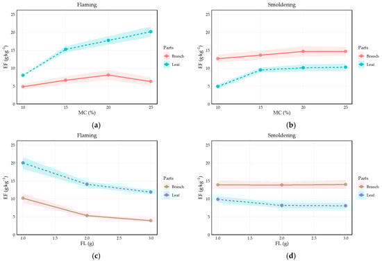
Figure 8. Variation in Impact Factors Released from Branches and Leaves with Moisture Content and Load under Flaming and Smoldering Burning Type: (a) Variation with moisture content under flaming combustion; (b) Variation with moisture content under smoldering combustion; (c) Variation with load under flaming combustion; (d) Variation with load under smoldering combustion.

Table 5 summarizes the variance components of the linear mixed-effects model (species random intercept and residual variance).

Table 5. LMM variance components (minimal).

Component	Variance	SD	ICC
Species (random intercept)	0.003506	0.0592	0.0120
Residual	0.288200	0.5369	/

Model includes a random intercept $\mathrm{u}\left\{0,\mathrm{S}\mathrm{p}\mathrm{e}\mathrm{c}\mathrm{i}\mathrm{e}\mathrm{s}\left(\mathrm{j}\right)\right\}$. Marginal/conditional R² = 0.567/0.572. The final fixed-effects structure was:

$$\mathrm{l}\mathrm{o}\mathrm{g}\left(\mathrm{E}\mathrm{F}\right)={\beta }_0+{\beta }_1\mathrm{z}\mathrm{F}\mathrm{L}+{\beta }_2\mathrm{z}\mathrm{M}\mathrm{C}+{\beta }_3\mathrm{z}{\mathrm{M}\mathrm{C}}^2+\mathrm{P}\mathrm{a}\mathrm{r}\mathrm{t}+\mathrm{B}\mathrm{T}+\mathrm{P}\mathrm{a}\mathrm{r}\mathrm{t}\times \mathrm{B}\mathrm{T}+\mathrm{z}\mathrm{M}\mathrm{C}\times \mathrm{P}\mathrm{a}\mathrm{r}\mathrm{t}+\mathrm{u}\left\{0,\mathrm{S}\mathrm{p}\mathrm{e}\mathrm{c}\mathrm{i}\mathrm{e}\mathrm{s}\left(\mathrm{j}\right)\right\}+\mathsf{\epsilon }$$

(7)

where:

$$\mathrm{z}\mathrm{X}={\displaystyle \frac{(\mathrm{X}-\mu \mathrm{X})}{\sigma \_\mathrm{X}}}$$

(8)

$$\mathrm{u}\left\{0,\mathrm{S}\mathrm{p}\mathrm{e}\mathrm{c}\mathrm{i}\mathrm{e}\mathrm{s}\left(\mathrm{j}\right)\right\}\sim \mathrm{N}(0,0.003506)$$

(9)

ε∼N(0, 0.288200)

(10)

All metrics are out-of-fold using the fixed-effects component. Lower RMSE/MAE is better.

3.2.3. Performance of GBM on EF

The GBM benchmark achieved 5-fold CV R² = 0. 665 with RMSE = 3.616 and MAE = 2.563, broadly matching the LMM’s out-of-foldR2. Relative influence ranked predictors as BT (34.26%), Part (31.04%), MC (18.72%), and FL (15.98%). Thus, while GBM captures potential nonlinearity and higher-order interactions, the variable importance pattern aligns with the LMM, reinforcing BT and Part as the primary drivers of EF, followed by MC and FL.

4. Discussion

Remote-sensing analyses of typical Siberian forest fires estimate ground-level aerosol emissions at 0.1–0.7 t/hm², with total particulate matter comprising roughly 1%–7% of the biomass consumed [41,42]. These values are markedly lower than ours; synthesizing data from indoor burning experiments on eucalyptus forests, grasses, and straw shows that their emissions, when transformed, either lie within or exceed our observed range [43,44,45,46]. However, in certain instances, individual observations are markedly higher than our measured values [47]. We ascribe these discrepancies to heterogeneity in PM_2.5 distributions driven by differences in spatial structure and transport dynamics [42,48]. In reality, PM_2.5 distributions deviate markedly from idealized assumptions, evolving through complex diffusion and transport processes; a fraction is lofted as atmospheric aerosols that scatter light and reduce visibility [49]. While the airborne fraction is captured in remote-sensing imagery and converted to emission estimates, a substantial share of PM_2.5 deposits to soils and thus escapes detection; moreover, PM_2.5 interacts with forest vegetation—studies show that plant leaves adsorb smoke-borne particulates [50], which further reduces the fraction detectable by remote sensing; in addition, plants subjected to biotic or abiotic stress can emit biogenic volatile organic compounds (BVOCs) [51].

To explain the irregular branch curve behavior observed for species other than CMM, we hypothesize that difficulty standardizing branch diameters in our broad-leaved shrub samples—which do not exhibit synchronous annual leaf shedding—together with the practical inability, despite excluding visibly distinct twigs, to guarantee that all combusted branches originated in the same year (hence variation in wood composition), contributed to the effect; prior work has shown that wood composition and fuel diameter can strongly influence emission factors [52].

Although increasing fuel load generally raises total PM_2.5, excessive loading can exert a counteracting influence [53]; accordingly, the PM_2.5 emission factor declines as load increases and its marginal change tapers—a pattern reported by other experimental studies [45]—and a plausible mechanism is that higher loading elevates combustion temperature and efficiency, promoting more complete burning and thus reducing solid-particle release per unit mass. Based on our experimental observations, variables such as fuel diameter may exert a more pronounced influence on emission factors than the interactive effects between branches and other predictors. In contrast to the heterogeneity observed in branch data, leaf emission factors exhibit a more structured and predictable sensitivity to continuous drivers—specifically fuel load and moisture content. This trend underscores the dominant role of organ-specific traits in modulating emission profiles, as further evidenced by the robust interactions identified in our mixed-effects framework.

Regarding the impact of moisture content (MC) on emission factors, previous studies that did not distinguish between plant organs generally offered the following explanation: high fuel moisture leads to a reduction in combustion temperature, which subsequently lowers the Modified Combustion Efficiency (MCE). Given that MCE is typically inversely correlated with EF, increasing moisture is expected to elevate particulate emissions [43,54]. In our analysis, if the focus remains solely on the ANOVA or StepAIC results, a similar generalized interpretation might be reached. However, the LMM results and data visualizations reveal a more nuanced reality: the response of branch tissues to moisture is relatively stable and less pronounced. In fact, the most significant driver of emission variability is the interaction between moisture content and leaf tissues (β = 0.8170), which serves as the primary engine for the observed EF spikes at higher moisture levels. This finding underscores the critical importance of organ-specific differentiation when constructing predictive models for shrub fire emissions.

Mechanistically, this organ-specific sensitivity is rooted in fuel thermal degradation kinetics: while MC acts as a “heat sink” that lowers the adiabatic flame temperature, it also shifts the pyrolysis pathways of leaf-based cellulose and lignin [55]. For leaves, elevated moisture effectively “widens” the smoldering window by prolonging the dehydration and carbonization stages, leading to a massive release of incomplete combustion intermediates as aerosols. This finding underscores the critical importance of organ-specific differentiation and synergistic interactions when constructing predictive models for shrub fire emissions.

When smoldering is compared with flaming, the smoldering curve is smoother while the flaming curve is markedly steeper; because partially unburned, combustible constituents are present during particle release and their rates and concentrations vary with fuel load and moisture, the absence of flaming in smoldering minimizes impacts on these constituents and compresses between-group variability, whereas flaming consumes them to degrees that differ with release dynamics, thereby amplifying variation in emission factors.

As anticipated, branches behaved differently under flaming versus smoldering—with visibly greater smoke in smoldering—and, consistent with PM_2.5 emission experiments during planned burns in southern Australian eucalyptus forests, the median smoldering EF substantially exceeded that under flaming, by roughly a factor of two [56], a difference attributed to contrasting combustion regimes (glowing-char combustion versus pyrolysis) that alter PM_2.5 magnitude and composition such that the biological toxicity of flaming smoke exceeds that of smoldering [55,57]; moreover, prior work shows that higher PM_2.5 emission factors are associated with lower combustion efficiency [43], implying more efficient branch combustion under flaming.

Contrary to reports that smoldering typically yields higher PM_2.5 emission factors than flaming, our data show that leaf EF actually decreased under smoldering. We attribute this discrepancy chiefly to experimental design differences in the cited study. Specifically, key variables were not held constant in their research, where flaming was tested on fine fuels (<6 mm) while smoldering was conducted on coarse fuels (>50 mm). This suggests that fuel size, rather than the combustion mode alone, acted as the primary driver for their observed results. Mechanistically, flaming proceeds through multiple stages that generate distinct compounds and often lead to uneven burning [55,58], whereas smoldering is governed by pyrolysis (dehydration → cellulose-fiber decomposition → wood decomposition) whose average dehydration rate, onset temperature, and decomposition rates of cellulose and lignin vary by species [59], potentially explaining leaf–branch contrasts under smoldering; moreover, some studies report EFs substantially higher than ours under ostensibly comparable conditions [47], suggesting that smoldering intensity in our setup may have been greater and thus altered the pyrolysis regime; to our knowledge, no study has directly compared branch and leaf combustion across methods, and we therefore posit that the “anomalous” branch-smoldering behavior may reflect formation of larger solids (rather than PM_2.5) removed by the size-cut, underscoring the need to disentangle combustion-method × fuel-property interactions—particularly the roles of fuel shape and composition.

Removing any pairwise interaction increased AIC (ΔAIC ≥ 7.9, up to 609.2), indicating that interactions are indispensable for fit; together with stable out-of-sample performance and a GBM benchmark of R² = 0.665, the case for retaining the full two-way specification is both necessary and justified, as the variable-importance ordering is likewise similar: BT 34.3% > PP 31.0% > MC 18.7% > FL 16.0%—implying that nonlinearity is present but limited and that the dominant structure is captured by second-order interactions with modest curvature, while LMM/OLS matches GBM performance yet affords more direct mechanistic interpretability.

The marginal AIC increase (ΔAIC = 10) falls within Burnham & Anderson’s “weak evidence” range [60], implying that the optimized model does not statistically outperform the original; moreover, the negligible changes in adjusted R² and residual standard error (RSE) further support prioritizing the initial model’s theoretical coherence over minor statistical fluctuations.

Because excluding moisture content interactions or organ-specific coefficients in the stepAIC-optimized model conflicts with established combustion dynamics, we retained moisture interactions and organ-specific effects in the a prior framework—even when AIC gains were marginal—to preserve biological plausibility and avoid misspecification; this stance is reinforced by data constraints (n = 1008; MC 10%–40%) that plausibly reduce power to detect curvature and cross-terms, a setting where stepwise selection is known to be unstable and biased [61], so a hybrid approach balancing information criteria with domain knowledge is warranted.

Our triangulation across models supports this position: within the two-way candidate space, AIC screening favored retaining all pairwise interactions (minimum ΔAIC = 7.9; up to 609.2), indicating that interactions materially improve fit rather than merely inflate complexity; the LMM on log(EF) with a species random intercept (1|Species) yields interpretable multiplicative effects (FL × 1.283/SD; MC × 0.856/SD; MC² × 0.907; Leaf × 3.52; Smoldering × 2.33; Leaf × Smoldering × 0.25; MC × Leaf × 2.26/SD) with tight CIs and a small species-level ICC (≈0.012), and its out-of-sample performance remains stable in both five-fold CV (R² = 0.662) and LOSO (R² = 0.640; Table 6 and Table 7). Given the multi-source variability of biomass-burning emission factors (EF) and the high noise inherent to wildfire-smoke systems [62,63], cross-validated R² values in the 0.62–0.67 range should be viewed as strong out-of-sample performance [64]. The EF is influenced by many sources of variation—differences in fuel morphology and composition, within- and between-sample moisture heterogeneity, branch diameter and organ structure, transitions between flaming and smoldering and ignition conditions, and sampling/filter-weighing errors—which together limit the theoretical ceiling for explainability. We also used k-fold cross-validation and leave-one-species-out (LOSO) validation, both stricter tests of generalization; under LOSO, R² remained approximately 0.64, indicating stable generalization rather than chance fit. This interpretation is consistent with wildfire-related PM_2.5 models that typically report CV-R² around 0.6–0.7 and with reviews identifying cross-fuel/combustion EF variability as a dominant source of uncertainty [65,66,67]. Under the current data characteristics and noise level, treating 0.62–0.67 as a strong signal is reasonable and conservative. In parallel, the GBM—a black-box benchmark that implicitly captures nonlinearity and higher-order interactions—achieves essentially the same predictive accuracy (R² = 0.665), and its relative influence ordering mirrors the LMM (BT 34.3% > Part 31.0% > MC 18.7% > FL 16.0%), indicating that any additional nonlinearity beyond two-way interactions plus modest MC curvature is limited, so retaining mechanistically motivated terms does not compromise—and may enhance—interpretability without sacrificing performance.

Table 6. LMM out-of-sample performance (original scale; minimal).

Setting	RMSE	MAE	R2
5-fold CV	0.01036	0.007579	0.6618
LOSO (leave-one-species-out)	0.01061	0.007784	0.6402
In-sample (fixed effects)	0.01029	0.007531	0.6686

Table 7. GBM relative influence (variable importance).

Predictor	Relative Influence (%)
BT	34.26
Part	31.04
MC	18.72
FL	15.98

5. Conclusions

Following controlled indoor ignitions, we quantified PM_2.5 emission factors (EFs) for seven common shrubs in the Liangshui region, addressing the question of whether interspecific variation necessitates species-specific modeling. The central EF range was 12 ± 5 g·kg⁻¹ (≈7–17 g·kg⁻¹) covering 68% of observations, with modest between-species differences (species-level ICC ≈ 0.012) but pronounced within-species organ contrasts (leaves vs. non-leaf tissues). These results confirm that a unified framework is statistically sufficient for these ecologically dominant taxa.

Across models, results converged on the same structure, revealing the quantitative dominance of combustion mode and plant organs over other variables. Combustion mode and plant organ dominated EFs, with a strong negative Leaf × Smoldering interaction—relative to the baseline (non-leaf × flaming), branches/non-leaf showed smoldering > flaming, whereas leaves showed the reverse (smoldering < flaming), so the combined effect for Leaf under smoldering was ≈2.06× baseline rather than the naive product of main effects; fuel load was positively associated with EFs (an approximately 28% increase for every one standard deviation (SD) increase), moisture content was on average negative (≈−14% per 1 SD) with mild curvature (MC² multiplier ≈ 0.907), and the moisture slope was organ-specific such that within 10%–40% MC, increasing moisture could fail to reduce—or even raise—EF for leaves. This specifically clarifies the complex non-linear and synergistic interactions between physical fuel traits.

A model comparison supports these conclusions: AIC screening favored retaining all pairwise interactions (minimum ΔAIC = 7.9; up to 609.2); an LMM on log(EF) with a species random intercept (1|Species) yielded interpretable multiplicative effects and stable out-of-sample performance (5-fold R²_(orig) = 0.662; LOSO R²_(orig) = 0.640), and a GBM achieved essentially the same accuracy (R² = 0.665) and the same importance ordering (BT > Part > MC > FL), corroborating that additional nonlinearity beyond two-way interactions plus modest MC curvature is limited.

Practically, these findings prioritize avoiding smoldering conditions and actively managing leafy fuels, tailoring moisture strategies by organ, and reducing fuel load where feasible. By shifting from “species classification” to “component management,” these insights provide a mechanistic bridge for more precise fire-risk assessments. Overall, EF variation is governed primarily by organ- and mode-specific interactions with limited nonlinearity, and interpretable statistical models and GBMs deliver comparable predictive capacity that supports actionable fire management guidance for this region.

While this study provides a high-resolution predictive framework based on controlled laboratory conditions, we acknowledge the inherent challenges in extrapolating these results to large-scale, stochastic wildfire scenarios. Laboratory ignitions allow for the precise isolation of individual variable effects—such as the identified non-linear moisture thresholds and organ-specific interactions—which are often obscured by the extreme scales and environmental turbulence of real-world wildfires. We recognize that the emission factors (EFs) derived under stationary laboratory settings may not be identical to those produced during landscape-scale conflagrations, where fire–weather feedback loops and plume dynamics significantly alter combustion efficiency. However, given that current remote sensing and field-based sensing techniques often struggle to resolve the true particulate output of massive, opaque fire fronts, our laboratory-derived data serves as a critical verified baseline. Future research should focus on cross-scale validation using bridge-scale prescribed burns to further refine the correspondence functions between controlled simulations and complex wilderness fire behavior.

References

- Fernandes, P.M.; Botelho, H.S. A review of prescribed burning effectiveness in fire hazard reduction. Int. J. Wildland Fire 2003, 12, 117–128. [Google Scholar] [CrossRef]
- McCaw, W.L. Managing forest fuels using prescribed fire—A perspective from southern Australia. For. Ecol. Manag. 2013, 294, 217–224. [Google Scholar] [CrossRef]
- Alcaniz, M.; Outeiro, L.; Francos, M.; Ubeda, X. Effects of prescribed fires on soil properties: A review. Sci. Total Environ. 2018, 613–614, 944–957. [Google Scholar] [CrossRef]
- San Emeterio, L.; Múgica, L.; Ugarte, M.D.; Goicoa, T.; Canals, R.M. Sustainability of traditional pastoral fires in highlands under global change: Effects on soil function and nutrient cycling. Agric. Ecosyst. Environ. 2016, 235, 155–163. [Google Scholar] [CrossRef]
- Augustine, D.J.; Brewer, P.; Blumenthal, D.M.; Derner, J.D.; von Fischer, J.C. Prescribed fire, soil inorganic nitrogen dynamics, and plant responses in a semiarid grassland. J. Arid. Environ. 2014, 104, 59–66. [Google Scholar] [CrossRef]
- Luterbacher, J.; Dietrich, D.; Xoplaki, E.; Grosjean, M.; Wanner, H. European seasonal and annual temperature variability, trends, and extremes since 1500. Science 2004, 303, 1499–1503. [Google Scholar] [CrossRef] [PubMed]
- Abram, N.J.; Henley, B.J.; Sen Gupta, A.; Lippmann, T.J.R.; Clarke, H.; Dowdy, A.J.; Sharples, J.J.; Nolan, R.H.; Zhang, T.R.; Wooster, M.J.; et al. Connections of climate change and variability to large and extreme forest fires in southeast Australia. Commun. Earth Environ. 2021, 2, 17. [Google Scholar] [CrossRef]
- Johnston, J.D.; Bailey, J.D.; Dunn, C.J.; Lindsay, A.A. Historical fire-climate relationships in contrasting interior pacific northwest forest types. Fire Ecol. 2017, 13, 18–36. [Google Scholar] [CrossRef]
- Certini, G. Effects of fire on properties of forest soils: A review. Oecologia 2005, 143, 1–10. [Google Scholar] [CrossRef]
- Stohl, A.; Berg, T.; Burkhart, J.F.; Fjæraa, A.M.; Forster, C.; Herber, A.; Hov, O.; Lunder, C.; McMillan, W.W.; Oltmans, S.; et al. Arctic smoke: Record high air pollution levels in the European Arctic due to agricultural fires in Eastern Europe in spring 2006. Atmos. Chem. Phys. 2007, 7, 511–534. [Google Scholar] [CrossRef]
- Liu, Y.; Heilman, W.E.; Potter, B.E.; Clements, C.B.; Jackson, W.A.; French, N.H.F.; Goodrick, S.L.; Kochanski, A.K.; Larkin, N.K.; Lahm, P.W.; et al. Recent Advances in Wildland Fire Smoke Dynamics Research in the United States. Atmosphere 2025, 16, 1221. [Google Scholar] [CrossRef]
- Solomon, S.; Qin, D.; Manning, M.; Chen, Z.; Marquis, M.; Averyt, K.B.; Tignor, M.; Miller, H.L. The Physical Science Basis: Contribution of Working Group I to the Fourth Assessment Report of the Intergovernmental Panel on Climate Change. In IPCC Fourth Assessment Report (AR4); Cambridge University Press: Cambridge, UK; New York, NY, USA, 2007; Volume 18, pp. 95–123. Available online: http://www.ipcc.ch/publications_and_data/publications_ipcc_fourth_assessment_report_wg1_report_the_physical_science_basis.htm (accessed on 10 December 2025).
- Guo, F.; Hu, H.; Peng, X. Estimation of Gases Released from Shrubs, Herbs and Litters Layer of Different Forest Types in Daxing’ an Mountains by Forest Fires from 1980 to 2005. Sci. Silvae Sin. 2010, 46, 78–83. [Google Scholar]
- Brey, S.J.; Ruminski, M.; Atwood, S.A.; Fischer, E.V. Connecting smoke plumes to sources using Hazard Mapping System (HMS) smoke and fire location data over North America. Atmos. Chem. Phys. 2018, 18, 1745–1761. [Google Scholar] [CrossRef]
- Zu, K.; Tao, G.; Long, C.; Goodman, J.; Valberg, P. Long-range fine particulate matter from the 2002 Quebec forest fires and daily mortality in Greater Boston and New York City. Air Qual. Atmos. Health 2016, 9, 213–221. [Google Scholar] [CrossRef] [PubMed]
- Afrin, S.; Garcia-Menendez, F. Potential impacts of prescribed fire smoke on public health and socially vulnerable populations in a Southeastern US state. Sci. Total Environ. 2021, 794, 10. [Google Scholar] [CrossRef]
- Cascio, W.E. Wildland fire smoke and human health. Sci. Total Environ. 2018, 624, 586–595. [Google Scholar] [CrossRef] [PubMed]
- Shou, Y.K.; Huang, Y.L.; Zhu, X.Z.; Liu, C.Q.; Hu, Y.; Wang, H.H. A review of the possible associations between ambient PM2.5 exposures and the development of Alzheimer’s disease. Ecotox. Environ. Safe 2019, 174, 344–352. [Google Scholar] [CrossRef] [PubMed]
- Aguilera, R.; Corringham, T.; Gershunov, A.; Benmarhnia, T. Wildfire smoke impacts respiratory health more than fine particles from other sources: Observational evidence from Southern California. Nat. Commun. 2021, 12, 8. [Google Scholar] [CrossRef]
- Arriagada, N.B.; Palmer, A.J.; Bowman, D.; Morgan, G.G.; Jalaludin, B.B.; Johnston, F.H. Unprecedented smoke-related health burden associated with the 2019–20 bushfires in eastern Australia. Med. J. Aust. 2020, 2, 282–283. [Google Scholar] [CrossRef]
- Arroyo, L.A.; Pascual, C.; Manzanera, J.A. Fire models and methods to map fuel types: The role of remote sensing. For. Ecol. Manag. 2008, 256, 1239–1252. [Google Scholar] [CrossRef]
- Souane, A.A.; Khurram, A.; Huang, H.; Shu, Z.; Feng, S.J.; Belgherbi, B.; Wu, Z.Y. Utilizing Machine Learning and Geospatial Techniques to Evaluate Post-Fire Vegetation Recovery in Mediterranean Forest Ecosystem: Tenira, Algeria. Forests 2025, 16, 25. [Google Scholar] [CrossRef]
- Cortés-Cabrera, H.E.; Jurado, E.; Pompa-García, M.; Aguirre-Calderón, O.A.; Pando-Moreno, M.; González-Tagle, M.A. Efecto de los incendios y la elevación en la regeneración de Pinus hartwegii Lindl. en el noreste de México. Rev. Chapingo Ser. Cienc. For. Ambiente 2018, 24, 197–205. [Google Scholar] [CrossRef]
- Clinton, N.E.; Gong, P.; Scott, K. Quantification of pollutants emitted from very large wildland fires in Southern California, USA. Atmos. Environ. 2006, 40, 3686–3695. [Google Scholar] [CrossRef]
- Wang, W.; Du, H.; Xiao, L.; Zhang, J.; Zhong, Z.; Zhou, W.; Zhang, B.; Wang, H.H. Plant Composition and Stand Structure Characteristics of Three Forest Types in the Liangshui Nature Reserve. Sci. Silvae Sin. 2019, 55, 166–176. [Google Scholar]
- Coen, J. Some Requirements for Simulating Wildland Fire Behavior Using Insight from Coupled Weather-Wildland Fire Models. Fire 2018, 1, 18. [Google Scholar] [CrossRef]
- Ziegler, J.P.; Hoffman, C.; Battaglia, M.; Mell, W. Spatially explicit measurements of forest structure and fire behavior following restoration treatments in dry forests. For. Ecol. Manag. 2017, 386, 1–12. [Google Scholar] [CrossRef]
- Price, O.F.; Rahmani, S.; Samson, S. Particulate Levels Underneath Landscape Fire Smoke Plumes in the Sydney Region of Australia. Fire 2023, 6, 16. [Google Scholar] [CrossRef]
- Simmons, J.B.; Paton-Walsh, C.; Mouat, A.P.; Kaiser, J.; Humphries, R.S.; Keywood, M.; Griffith, D.W.T.; Sutresna, A.; Naylor, T.; Ramirez-Gamboa, J. Bushfire smoke plume composition and toxicological assessment from the 2019–2020 Australian Black Summer. Air Qual. Atmos. Health 2022, 15, 2067–2089. [Google Scholar] [CrossRef]
- Joel, S.L. Biomass Burning: Its History, Use, and Distribution and Its Impact on Environmental Quality and Global Climate. In Global Biomass Burning: Atmospheric, Climatic, and Biospheric Implications; MIT Press: Cambridge, MA, USA, 1991; pp. 3–21. [Google Scholar]
- Hays, M.D.; Fine, P.M.; Geron, C.D.; Kleeman, M.J.; Gullett, B.K. Open burning of agricultural biomass: Physical and chemical properties of particle-phase emissions. Atmos. Environ. 2005, 39, 6747–6764. [Google Scholar] [CrossRef]
- Junquera, V.; Russell, M.M.; Vizuete, W.; Kimura, Y.; Allen, D. Wildfires in eastern Texas in August and September 2000: Emissions, aircraft measurements, and impact on photochemistry. Atmos. Environ. 2005, 39, 4983–4996. [Google Scholar] [CrossRef]
- Jin, Q.F.; Wang, W.W.; Zheng, W.X.; Innes, J.L.; Wang, G.Y.; Guo, F.T. Dynamics of pollutant emissions from wildfires in Mainland China. J. Environ. Manag. 2022, 318, 19. [Google Scholar] [CrossRef]
- Wang, K. Carbon Stability Characteristics and Driving Mechanisms of Forest Biomass in Northeast China. Ph.D. Thesis, Northeast Institute of Geography and Agroecology, CAS, Changchun, China, 2024. [Google Scholar]
- Jin, Y.Q.; Liu, C.G.; Qian, S.S.; Luo, Y.Q.; Zhou, R.W.; Tang, J.W.; Bao, W.K. Root/shoot ratio Understory vegetation. Sci. Total Environ. 2022, 804, 9. [Google Scholar] [CrossRef]
- Yang, X.; Guo, Y.; Mohhamot, A.; Liu, H.; Ma, W.; Yu, S.; Tang, Z. Distribution of biomass in relation to environments in shrublands of temperate China. Chin. J. Plant Ecol. 2017, 41, 22–30. [Google Scholar]
- Abbas, K.; Souane, A.A.; Ahmad, H.; Suita, F.; Shu, Z.; Huang, H.; Wang, F. Correlating Fire Incidents with Meteorological Variables in Dry Temperate Forest. Forests 2025, 16, 26. [Google Scholar] [CrossRef]
- Dasdemir, I.; Aydin, F.; Ertugrul, M. Factors Affecting the Behavior of Large Forest Fires in Turkey. Environ. Manag. 2021, 67, 162–175. [Google Scholar] [CrossRef] [PubMed]
- Josephson, A.J.; Castaño, D.; Koo, E.; Linn, R.R. Zonal-Based Emission Source Term Model for Predicting Particulate Emission Factors in Wildfire Simulations. Fire Technol. 2021, 57, 943–971. [Google Scholar] [CrossRef]
- Wu, Z.Y.; Hasham, A.; Zhang, T.B.; Gu, Y.; Lu, B.B.; Sun, H.; Shu, Z. Analysis of PM2.5 Concentration Released from Forest Combustion in Liangshui National Natural Reserve, China. Fire 2024, 7, 15. [Google Scholar] [CrossRef]
- Samsonov, Y.N.; Koutsenogii, K.P.; Makarov, V.I.; Ivanov, A.V.; Ivanov, V.A.; McRae, D.J.; Conard, S.G.; Baker, S.P.; Ivanova, G.A. Particulate emissions from fires in central Siberian Scots pine forests. Can. J. For. Res.-Rev. Can. Rech. For. 2005, 35, 2207–2217. [Google Scholar] [CrossRef]
- Parrington, M.; Whaley, C.H.; French, N.H.F.; Buchholz, R.R.; Pan, X.H.; Wiedinmyer, C.; Hyer, E.J.; Kondragunta, S.; Kaiser, J.W.; Di Tomaso, E.; et al. Biomass burning emission estimation in the MODIS era: State-of-the-art and future directions. Elem.-Sci. Anthrop. 2025, 13, 23. [Google Scholar] [CrossRef]
- Dong, T.T.T.; Stock, W.D.; Callan, A.C.; Strandberg, B.; Hinwood, A.L. Emission factors and composition of PM2.5 from laboratory combustion of five Western Australian vegetation types. Sci. Total Environ. 2020, 703, 134796. [Google Scholar] [CrossRef]
- Ni, H.Y.; Han, Y.M.; Cao, J.J.; Chen, L.W.A.; Tian, J.; Wang, X.L.; Chow, J.C.; Watson, J.G.; Wang, Q.Y.; Wang, P.; et al. Emission characteristics of carbonaceous particles and trace gases from open burning of crop residues in China. Atmos. Environ. 2015, 123, 399–406. [Google Scholar] [CrossRef]
- Alves, C.; Vicente, A.; Nunes, T.; Gonçalves, C.; Fernandes, A.P.; Mirante, F.; Tarelho, L.; de la Campa, A.M.S.; Querol, X.; Caseiro, A.; et al. Summer 2009 wildfires in Portugal: Emission of trace gases and aerosol composition. Atmos. Environ. 2011, 45, 641–649. [Google Scholar] [CrossRef]
- Ju, Y.; Yang, X.; Jin, Q.; Cai, Q.; Guo, F. Emission factor and main components of PM2.5 emitted from crop straw under different burning status. Acta Sci. Circumstantiae 2018, 38, 92–100. [Google Scholar]
- Yang, W.-Z.; Liu, G.; Li, J.-H.; Xu, H.; Wu, D. Emission of Particulate Matter, Organic and Elemental Carbon from Burning of Fallen Leaves. Environ. Sci. 2015, 36, 1202–1207. [Google Scholar]
- Liu, Q.; Liu, Z.; Li, Y.; Sun, Y.; Liu, Y.; Huang, Y. Study on reduction characteristics of PM2.5 and PM10 in urban parks based on DSM:a case study of Nanchang People’s Park. Acta Agric. Univ. Jiangxiensis 2024, 46, 173–183. [Google Scholar]
- Tao, J.; Zhang, L.M.; Cao, J.J.; Zhang, R.J. A review of current knowledge concerning PM2.5 chemical composition, aerosol optical properties and their relationships across China. Atmos. Chem. Phys. 2017, 17, 9485–9518. [Google Scholar] [CrossRef]
- Zheng, W.X.; Ma, Y.F.; Tigabu, M.; Yi, Z.G.; Guo, Y.X.; Lin, H.C.; Huang, Z.Y.; Guo, F.T. Capture of fire smoke particles by leaves of Cunninghamia lanceolata and Schima superba, and importance of leaf characteristics. Sci. Total Environ. 2022, 841, 11. [Google Scholar] [CrossRef]
- Guo, Y.X.; Ma, Y.F.; Zhu, Z.P.; Tigabu, M.; Marshall, P.; Zhang, Z.; Lin, H.C.; Huang, Z.Y.; Wang, G.Y.; Guo, F.T. Release of biogenic volatile organic compounds and physiological responses of two sub-tropical tree species to smoke derived from forest fire. Ecotox. Environ. Safe 2024, 275, 12. [Google Scholar] [CrossRef]
- Leenhouts, B. Assessment of Biomass Burning in the Conterminous United States. Conserv. Ecol. 1998, 2, 1. [Google Scholar] [CrossRef]
- Ning, J.; Zhang, Y.; Yuan, S.; Yu, H.; Di, X.; Yang, G. A Review of PM2.5 Emissions from Wildland Fires: Recent Advances. World For. Res. 2021, 34, 52–57. [Google Scholar] [CrossRef]
- Tang, S.Y.; Yin, S.N.; Shan, Y.L.; Yu, B.; Cui, C.X.; Cao, L.L. The Characteristics of Gas and Particulate Emissions from Smouldering Combustion in the Pinus pumila Forest of Huzhong National Nature Reserve of the Daxing’an Mountains. Forests 2023, 14, 14. [Google Scholar] [CrossRef]
- Koss, A.R.; Sekimoto, K.; Gilman, J.B.; Selimovic, V.; Coggon, M.M.; Zarzana, K.J.; Yuan, B.; Lerner, B.M.; Brown, S.S.; Jimenez, J.L.; et al. Non-methane organic gas emissions from biomass burning: Identification, quantification, and emission factors from PTR-ToF during the FIREX 2016 laboratory experiment. Atmos. Chem. Phys. 2018, 18, 3299–3319. [Google Scholar] [CrossRef]
- Reisen, F.; Meyer, C.P.; Weston, C.J.; Volkova, L. Ground-Based Field Measurements of PM2.5 Emission Factors From Flaming and Smoldering Combustion in Eucalypt Forests. J. Geophys. Res. Atmos. 2018, 123, 8301–8314. [Google Scholar] [CrossRef]
- Kim, Y.H.; King, C.; Krantz, T.; Hargrove, M.M.; George, I.J.; McGee, J.; Copeland, L.; Hays, M.D.; Landis, M.S.; Higuchi, M.; et al. The role of fuel type and combustion phase on the toxicity of biomass smoke following inhalation exposure in mice. Arch. Toxicol. 2019, 93, 1501–1513. [Google Scholar] [CrossRef] [PubMed]
- Lazaridis, M.; Latos, M.; Aleksandropoulou, V.; Hov, O.; Papayannis, A.; Torseth, K. Contribution of forest fire emissions to atmospheric pollution in Greece. Air Qual. Atmos. Health 2008, 1, 143–158. [Google Scholar] [CrossRef]
- Jin, S.; Song, Y.; Sun, C. Slow-Heating Pyrolysis Characteristics of 12 Herbaceous Fuels in Mao’ershan, Heilongjiang. Sci. Silvae Sin. 2012, 48, 101–108. [Google Scholar]
- Burnhan, K.P.; Anderson, D.R. Model selection and multi-model inference: A practical Information-theoretic approach. Technometrics 2002, 45, 181. [Google Scholar]
- Helmreich, J.E. Regression Modeling Strategies with Applications to Linear Models, Logistic and Ordinal Regression and Survival Analysis (2nd Edition). J. Stat. Softw. 2016, 70, 1–3. [Google Scholar] [CrossRef]
- Akagi, S.K.; Yokelson, R.J.; Wiedinmyer, C.; Alvarado, M.J.; Reid, J.S.; Karl, T.; Crounse, J.D.; Wennberg, P.O. Emission factors for open and domestic biomass burning for use in atmospheric models. Atmos. Chem. Phys. 2011, 11, 4039–4072. [Google Scholar] [CrossRef]
- Andreae, M.O. Emission of trace gases and aerosols from biomass burning—An updated assessment. Atmos. Chem. Phys. 2019, 19, 8523–8546. [Google Scholar] [CrossRef]
- Minh, V.T.T.; Tin, T.T.; Hien, T.T. PM2.5 Forecast System by Using Machine Learning and WRF Model, A Case Study: Ho Chi Minh City, Vietnam. Aerosol Air Qual. Res. 2021, 21, 17. [Google Scholar] [CrossRef]
- Geng, G.N.; Murray, N.L.; Tong, D.; Fu, J.S.; Hu, X.F.; Lee, P.; Meng, X.; Chang, H.H.; Liu, Y. Satellite-Based Daily PM2.5 Estimates During Fire Seasons in Colorado. J. Geophys. Res.-Atmos. 2018, 123, 8159–8171. [Google Scholar] [CrossRef] [PubMed]
- Swanson, A.; Holden, Z.A.; Graham, J.; Warren, D.A.; Noonan, C.; Landguth, E. Daily 1 km terrain resolving maps of surface fine particulate matter for the western United States 2003–2021. Sci. Data 2022, 9, 466. [Google Scholar] [CrossRef]
- Urbanski, S. Wildland fire emissions, carbon, and climate: Emission factors. For. Ecol. Manag. 2014, 317, 51–60. [Google Scholar] [CrossRef]
Disclaimer/Publisher’s Note: The statements, opinions and data contained in all publications are solely those of the individual author(s) and contributor(s) and not of MDPI and/or the editor(s). MDPI and/or the editor(s) disclaim responsibility for any injury to people or property resulting from any ideas, methods, instructions or products referred to in the content. |
© 2026 by the authors. Licensee MDPI, Basel, Switzerland. This article is an open access article distributed under the terms and conditions of the Creative Commons Attribution (CC BY) license.