Spatial Vertical Distribution of the Leaf Nitrogen Concentration in Young Cephalotaxus hainanensis

Abstract

Cephalotaxus hainanensis, a valuable medicinal and endangered conifer, requires scientific conservation and precision management to ensure the sustainable utilization of its genetic and ecological resources. Nitrogen (N) is a key nutrient that regulates plant growth and metabolism; rapid and accurate nitrogen diagnosis is vital for optimizing fertilization, reducing nutrient losses, and promoting healthy plant development. This study employed a combined approach integrating stepwise regression, correlation analysis, and Least Absolute Shrinkage and Selection Operator (LASSO) regression to identify leaf color features strongly correlated with leaf nitrogen content (LNC). A support vector regression (SVR) model, suitable for small-sample datasets, was then employed to accurately estimate LNC across canopy layers. Nine color variables were found to be highly associated with LNC, among which the Green Minus Blue index (GMB) consistently appeared across all correlation methods, demonstrating strong robustness and generality. Color features effectively reflected LNC variations among nitrogen treatments—especially between N1 and N4—and across canopy layers, with the most pronounced contrasts observed between upper and lower leaves. The Spearman-based SVR model revealed that the middle canopy maintained the highest and most stable LNC. However, the lower leaves were most sensitive to nitrogen deficiency, while the upper leaves were more sensitive to nitrogen excess. Comprehensive analysis identified N2 as the optimal nitrogen treatment, representing a balanced nutrient state. Overall, this study confirms the reliability of color features for LNC estimation and highlights the importance of vertical canopy LNC distribution in nitrogen diagnostics, providing a theoretical and methodological foundation for color-based nitrogen diagnosis and precision nutrient management in evergreen conifers.

1. Introduction

Cephalotaxus hainanensis contains abundant bioactive compounds such as alkaloids and lactones and shows the highest levels of anticancer activity-related compounds among species of the genus Cephalotaxus in China [1,2]. Owing to its remarkable medicinal value, the species has attracted considerable pharmacological interest. However, its natural populations are scarce [3] and have been classified as endangered. Demographic surveys indicate low survival rates of seedlings and saplings, resulting in limited regeneration and a declining population structure [4]. These constraints underscore the need for accurate, non-destructive nutrient diagnostics during the juvenile stage to promote healthy growth and support effective conservation management.

Nitrogen (N) is a fundamental nutrient regulating plant growth, photosynthesis, and metabolism. Within leaves, N supports photosynthetic machinery and cell wall construction, and approximately 75% of foliar N in mature leaves of higher plants is localized within chloroplasts, with more than half directly associated with photosynthesis [5,6,7]. Chlorophyll, the key photosynthetic pigment, captures light energy and converts it into chemical energy for plant growth [8]. Both traditional leaf color charts and modern image-based nutrient diagnostic techniques rely on the intrinsic relationship between chlorophyll content and leaf nitrogen concentration [9]. This relationship has been effectively quantified in various studies using advanced imaging approaches, such as UAV-based hyperspectral imagery [10,11], establishing a solid theoretical basis for applying low-cost RGB image analysis to nitrogen estimation. Accordingly, leaf color can serve as an intuitive and informative indicator of plant nitrogen status, enabling convenient, non-destructive monitoring under field conditions.

Compared with broadleaf species and crops, conifers—including C. hainanensis—exhibit distinctive morphological and physiological traits that influence nitrogen diagnostics. Conifer leaves typically have a linear or needle-like morphology with a high leaf mass per unit area, and a relatively large proportion of leaf nitrogen is allocated to non-photosynthetic proteins and storage compounds rather than to photosynthetic machinery [5]. These characteristics tend to weaken the responsiveness of leaf color or spectral indices to nitrogen variation, thereby increasing the difficulty of image-based nitrogen inversion. Moreover, studies on RGB image-based nitrogen estimation in conifer species remain scarce, particularly for rare or endangered trees, where limited sample availability further constrains methodological development and validation.

The vertical distribution of leaf nitrogen concentration (LNC) within plant canopies is inherently heterogeneous. To optimize nitrogen use efficiency, plants typically allocate more N to upper-canopy leaves to maximize photosynthetic capacity [12,13]. Soil nutrient availability, fertilization, and leaf age further regulate this vertical pattern [14,15]. For example, N application alters the vertical distribution of LNC in rice, with lower leaves being particularly sensitive [16]. The “productivity–leaf longevity hypothesis” emphasizes species-specific nitrogen strategies, whereby long-lived leaves sustain photosynthetic returns over extended lifespans, even under limited nutrient supply [5]. Despite these insights, the three-dimensional heterogeneity of LNC in trees, particularly conifers, remains poorly understood.

Recent progress in computer vision and digital imaging has facilitated the rapid, low-cost, and non-destructive monitoring of plant nutritional status [17]. However, most existing studies simplify canopy structure by averaging values, overlooking vertical heterogeneity and limiting diagnostic accuracy. To address this gap, the present study focuses on C. hainanensis and employs high-resolution leaf scanning combined with color index analysis and canopy partitioning. By examining vertical variations in leaf color and their relationship with nitrogen content, this study provides a reproducible framework for non-destructive nitrogen estimation in a rare conifer and offers novel insights into leaf nitrogen allocation patterns, which are relevant for both conservation and forest management.

2. Materials and Methods

2.1. Experimental Design

The experiment was conducted at the C. hainanensis cultivation and production base of the Hainan Academy of Forestry (110°28′46.08″ E, 19°51′55.94″ N). The trial was initiated in June 2021 using one-year-old C. hainanensis seedlings with the same growth status as experimental materials. Seedlings were cultivated in plastic pots (upper diameter: 36 cm; bottom diameter: 26 cm; height: 31.5 cm), with one seedling per pot. Each pot was filled with approximately 0.015–0.018 m³ of red soil (acidic) and amended with 500 g of well-decomposed organic sheep manure as a basal fertilizer. After a three-month acclimation period, urea (46% N) was applied as a topdressing at the beginning of each month. Four nitrogen application levels were established: 0, 5, 10, and 15 g·plant⁻¹·month⁻¹, designated as N1, N2, N3, and N4, respectively.

2.2. Data Acquisition

An initial survey of C. hainanensis seedlings was conducted in early June 2021, during which basic growth parameters, including plant height, ground diameter, and crown width, were recorded for all individuals. Subsequently, destructive sampling was conducted in May 2022, October 2022, and May 2023, resulting in a total of 63 samples. At each destructive sampling time point, the same growth parameters were re-measured to characterize the temporal changes in seedling growth status. In parallel, RGB images of all leaves were acquired using a conventional flatbed scanner (Smart Tank 520, HP Inc., Chongqing, China), which was employed exclusively to capture leaf color information in the RGB color space. During the final sampling in May 2023, leaves were further classified by dividing the height of each individual plant into three equal sections, which were labeled as upper, middle, and lower positions from the canopy top to the stem base, and leaf positions were clearly identified and recorded. Total leaf nitrogen concentration was determined using the semi-micro Kjeldahl method.

2.3. Image Feature Extraction

This study first used individual small branches as the basic analytical unit, performing segmentation and cropping with the Matrix Laboratory (version MATLAB R2022a, The MathWorks, Inc., Natick, MA, USA). Subsequently, the Excess Green minus Excess Red index (ExGR) was employed to extract branch regions [18]. For each extracted region, the mean values of the color components in the RGB, HSV, and CIELAB color spaces were calculated and denoted as R, G, B, H, S, V, L*, a*, and b*, respectively. Finally, by averaging the results across all branches of an individual plant, a set of plant-level color features was obtained.

The R, G, and B color components were normalized following the method of Lee and Lee [19] and Li et al. [20], denoted as r, g, and b, respectively, as shown in the following equations:

r = R/(R + G + B)

(1)

g = G/(R + G + B)

(2)

b = B/(R + G + B)

(3)

This study systematically reviewed the RGB color indices proposed in recent years (Table 1). All color indices were calculated using both the original R, G, and B components, as well as their normalized r, g, and b components. To distinguish the indices derived from the normalized values, the suffix “_X” was added to each corresponding index. In total, we extracted 55 color indices, which comprise the complete set of feature variables (Table 2).

Table 1. List of color indices (CIs) used in this study.

Abbreviation	Method of Calculation	Reference
GR	G/R	[21]
GB	G/B	[22]
I_KAW	(R − B)/(R + B)	[23]
NDI	(G − R)/(G + R)	[24]
NDYI	(G − B)/(G + B)	[25]
WI	(G − B)/(R − G)	[24]
VARI	(G − R)/(G + R − B)	[26]
DGBVI	((B − R))/((R + G + B))	[27]
GLI	(2G − R − B)/(2G + R + B)	[28]
MGRVI	(G2 − R2)/(G2 + R2)	[29]
MRBVI	(R2 − B2)/(R2 + B2)	[30]
RGBVI	(G2 − B × R)/(G2 + B × R)	[29]
MNGRVI	(G2 − G × R)/(G2 + G × R)	[30]
MNGRBVI	(B2 − G × R)/(B2 + G × R)	[30]
NID	128 × (((G − R)/(G + R)) + 1)	[31]
VEG	G/(RaB1−a), a = 0.667	[32]
ExG	2R − G − B	[24]
ExR	1.4R − G	[33]
ExB	1.4B − G	[34]
ExGR	ExG − ExR	[35]
CIVE	0.441R − 0.811G + 0.385B + 18.78745	[36]
COM1	ExG + CIVE + ExGR + VEG	[37]
MExG	1.262G − 0.884R − 0.311B	[38]
COM2	0.36ExG + 0.47CIVE + 0.17VEG	[39]
GMR	G − R	[21]
GMB	G − B	[40]
PCAI	0.994|R − B| + 0.961|G − B| + 0.914|G − R|	[41]
TCVI	(1.4 × (2R − 2B))/(2R − G − 2B + 255 × 0.4)	[42]
GRAY	0.2898R + 0.5870G + 0.1140B	[43]
DGCI	(((Hue − 60))/60 + (1 − Saturation) + (1 − Brightness))/3	[44]

Table 2. The complete set of feature variables.

Color Space		Color Indices	Number
RGB	Unnormalized	R, G, B, GR, GB, I_KAW, NDI, NDYI, WI, VARI, DGBVI, GLI, MGRVI, MRBVI, RGBVI, MNGRVI, MNGRBVI, NID, VEG, ExG, ExR, ExB, ExGR, CIVE, COM1, MExG, COM2, GMR, GMB, PCAI, TCVI, GRAY	32
	Normalized	r, g, b, ExG_X, ExR_X, ExB_X, ExGR_X, CIVE_X, COM1_X, MExG_X, COM2_X, GMR_X, GMB_X, PCAI_X, TCVI_X, GRAY_X	16
HSV		H, S, V, DGCI	4
CIELAB		L*, a*, b*	3
Total			55

2.4. Data Processing

2.4.1. Data Partitioning

All sample data were randomly divided into training and testing sets at a ratio of 8:2. As a result, the training set contained 51 samples, while the testing set included 12 samples.

2.4.2. Data Augmentation

The leaf color parameters exhibited a higher sensitivity to low LNCs, showing a pronounced variation gradient. As LNC increased, the leaf color response gradually reached saturation, with changes becoming less distinct. To stabilize data variance, the LNC values were log-transformed, followed by normalization of all variables.

To address the limitations of the small sample size and data distribution imbalance, which can hinder the model’s generalization capability, the Adaptive Synthetic for regression oversampling algorithm (ADASYNR) was applied to the training set for data augmentation [45]. Specifically, undersampling was performed on the high-nitrogen samples (with a ratio of 0.7), while oversampling was applied to the low-nitrogen samples (with a ratio of 4.2). This strategy effectively balanced the data distribution (Figure 1). Following augmentation, the training set was expanded to a total of 56 samples.

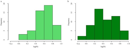
Figure 1. LNC distribution histogram. Original training data distribution (a). Training data distribution after ADASYNR (b).

2.4.3. Feature Selection

To address the severe multicollinearity observed among the 57 initially selected feature variables, a systematic variable screening strategy was employed (Figure 2). First, a preliminary selection was conducted using stepwise regression to reduce collinearity among variables. To minimize spurious correlations, the training dataset was evenly divided into two subsets. For each subset, five correlation analysis methods—Hilbert–Schmidt Independence Criterion (HSIC), Distance Correlation (DC), Copula Entropy (CE), Pearson correlation coefficient (Pearson), and Spearman’s rank correlation coefficient (Spearman)—were applied to evaluate the relationship between variables.

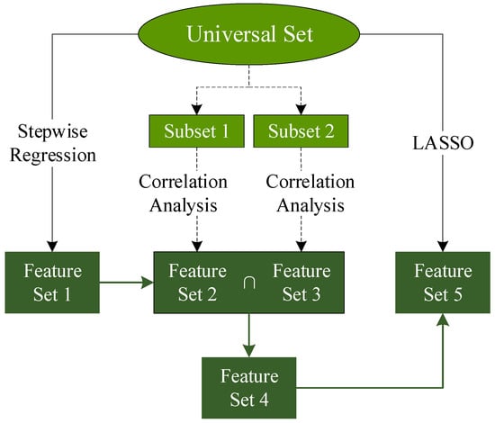
Figure 2. The flow chart of feature selection.

The intersection of the top 30 ranked variables from the two subsets was then extracted and further refined using Least Absolute Shrinkage and Selection Operator (LASSO) regression. This process yielded several sets of variables derived from different correlation-based methods (Table 3).

Table 3. Modeling formula for LNC.

Method	Formula	Number
HSIC	Log(N)~H + r + ExG + ExB + GMB + GB + RGBVI + MNGRBVI + DGBVI + DGCI + GMB_X + b*	12
DC	Log(N)~r + ExB + COM2 + GMB + GB + I_KAW + PCAI + DGCI + GMB_X + L* + b*	11
CE	Log(N)~S + V + r + b + GMB + PCAI + RGBVI + MNGRBVI + DGBVI + ExG_X	10
Pearson	Log(N)~R + S + V + b + ExB + GMB + GB + MRBVI + DGBVI + L*	10
Spearman	Log(N)~R + S + V + r + ExB + NDYI + GMB + MRBVI + TCVI + DGBVI + L* + b*	12

2.4.4. Model Construction and Parameter Optimization

Given that Support Vector Regression (SVR) models have demonstrated strong suitability for small-sample datasets [45,46], an SVR model was adopted to predict the LNC in this study. Parameter optimization was performed using leave-one-out cross-validation (LOOCV) in combination with a global search implemented through the Generalized Simulated Annealing (Gensa) algorithm. All modeling and analysis procedures were carried out in the R statistical environment (version 4.4.2; R Foundation for Statistical Computing, Vienna, Austria).

2.4.5. Model Evaluation

The coefficient of determination (R²), root mean square error (RMSE), and mean absolute error (MAE) were employed as evaluation metrics to assess model performance. The calculation formulas are as follows:

$${\mathrm{R}}^2=1-{\displaystyle \frac{{\sum }_{i=1}^n{(y_i-{\widehat{y}}_i)}^2}{{\sum }_{i=1}^n{(y_i-\overline{y})}^2}}$$

(4)

$$\mathrm{R}\mathrm{M}\mathrm{S}\mathrm{E}=\sqrt{{\displaystyle \frac{1}{n}}{\sum }_{i=1}^n{(y_i-{\widehat{y}}_i)}^2}$$

(5)

$$\mathrm{M}\mathrm{A}\mathrm{E}={\displaystyle \frac{1}{n}}{\sum }_{i=1}^n|y_i-{\widehat{y}}_i|$$

(6)

where $y_i$ and ${\widehat{y}}_i$ represent the observed and predicted values of the i-th sample, respectively; $\overline{y}$ denotes the average of all observed values; and n is the number of samples in the training or testing set.

3. Results

3.1. Feature Selection

In this study, feature dimensionality reduction was performed using a combined strategy integrating stepwise regression, correlation analysis, and LASSO regression. During the correlation analysis phase, five methods (CE, Pearson, Spearman, DC, and HSIC) were employed. Ultimately, 24 variables of relatively high importance were systematically identified (Figure 3). Specifically, the CE, Pearson, Spearman, DC, and HSIC methods selected 10, 10, 12, 11, and 12 variables, respectively (Table 3).

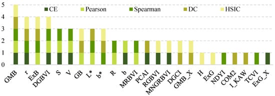
Figure 3. Variable set selected by five types of correlation.

A comparative analysis of the results revealed that the variable GMB was consistently selected by all five correlation-based methods, indicating its robustness and importance across multiple correlation metrics. In addition, eight other variables were selected by at least three of the five methods and were thus defined as high-frequency overlapping variables. Further statistical analysis showed that these eight high-frequency variables accounted for 50.00% (5/10), 70.00% (7/10), 66.67% (8/12), 54.54% (6/11), and 50.00% (6/12) of the variables selected by CE, Pearson, Spearman, DC, and HSIC, respectively, highlighting their consistent importance under diverse correlation measurement criteria.

3.2. Model Fitting

In this study, SVR models were combined with variables selected using various correlation analysis methods to predict LNC. The results showed that the variables selected by the Pearson and Spearman methods achieved strong predictive performance on both the training and testing datasets. Specifically, their testing performance was characterized by an R² > 0.8, RMSE < 0.3, and MAE < 0.24, indicating excellent generalization capability.

In contrast, the overall performance of the CE-, DC-, and HSIC-based models on the testing set was relatively lower. Among these three methods, the predicted performance on the testing set showed that the RMSE increased in the order of CE < HSIC < DC, the MAE increased in the order of DC < HSIC < CE, and the R² decreased in the order of DC > CE > HSIC. A comprehensive comparison of all evaluation metrics suggests that, although the DC-based model generalized better than those based on CE and HSIC, its performance remained inferior to the Pearson- and Spearman-based models. Moreover, the models derived from CE- and HSIC-selected variables exhibited evident underfitting on the testing dataset (Table 4).

Table 4. Model predicts performance for LNC.

Method	Training Set			Test Set
	RMSE	R2	MAE	RMSE	R2	MAE
HSIC	0.0768	0.9542	0.0286	0.3073	0.5844	0.2505
DC	0.0749	0.9576	0.0307	0.3097	0.7067	0.2461
CE	0.0846	0.9440	0.0339	0.3053	0.5878	0.2522
Pearson	0.0680	0.9675	0.0295	0.2959	0.8148	0.2308
Spearman	0.0422	0.9876	0.0195	0.2978	0.8117	0.2298

Further analysis of the distribution of selected variables (Figure 3) revealed that among the nine high-frequency overlapping variables, those screened by the Pearson and Spearman methods accounted for the highest proportion, followed by DC. At the same time, CE and HSIC have the lowest proportion. This distribution pattern was highly consistent with the model’s predictive performance, suggesting a potential association between the stability of variables and the model’s generalization capability.

Based on the above results, the Pearson and Spearman methods, which exhibited superior performance, were further selected for LNC inversion using scanned images collected during the third sampling campaign (October 2022). The LNC inverse was conducted separately for leaves from the upper, middle, and lower canopy positions. The inversion results from the three positions were then averaged and fitted against the measured nitrogen content (Figure 4).

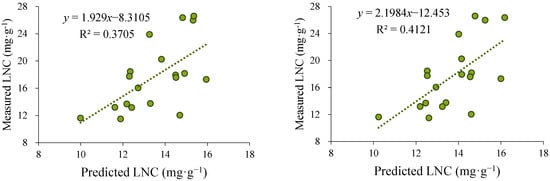
Figure 4. Comparison of the fitting results obtained using the Pearson and Spearman methods. The left panel presents the predicted values derived from the Pearson-based model, while the right panel displays those obtained from the Spearman-based model. Scatter plot of predicted versus observed leaf nitrogen concentration (LNC), with the solid line representing the fitted regression.

The results showed that the inversion outcomes obtained using the Spearman method exhibited a stronger correlation with the observed values, with an R² of 0.4121, which was higher than that of the Pearson method (0.3705). Therefore, the Spearman method was ultimately selected for LNC inversion across different canopy layers during the third sampling event, providing a reliable data foundation for subsequent analyses of the vertical nitrogen distribution pattern within the canopy.

3.3. Spatial Distribution of Leaf Color and LNC in C. hainanensis

3.3.1. Differences in Leaf Color Under Different Nitrogen Levels and Canopy Positions

This study explored the variation patterns of leaf color of C. hainanensis from two perspectives: nitrogen application levels and canopy positions. Analysis of variance (ANOVA) on LNC revealed limited variability among nitrogen treatments. Multiple comparison results indicated that only the N1 and N4 treatments differed significantly, while no significant differences were observed among the remaining treatments (Figure 5c). In contrast, leaf color exhibited more sensitive and complex responses to nitrogen application levels. Except for the B channel, significant differences were observed between N4 and N1, as well as between N4 and N2, across most color channels. However, the differences between N3 and the other treatments (N4, N1, N2) showed variations across color channels. Specifically, in the R channel of the RGB color space, N3 significantly differed from N2 but not from N4; in the H and a* channels, N3 significantly differed from N1 and N2 but not from N4; in the S, L*, and b* channels, N3 only significantly differed from N4; while in the V channel, no significant differences were found between N3 and any other treatment (Figure 5a).

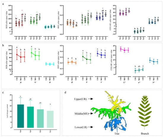
Figure 5. Differences in plant color under different nitrogen application levels. Error bars represent the standard errors of the means. Different letters indicate significant differences (p < 0.05), and unmarked letters indicate no significant differences. Differences in leaf color under different nitrogen application levels (a). Differences in leaf color among different leaf positions within the canopy (b). Differences in leaf nitrogen concentration under different nitrogen application levels (c). A schematic illustration of leaf positions within the canopy, which is not drawn to scale in (d). Leaf positions were determined by dividing the plant height into three equal sections: upper (UR), middle (ME), and lower (LR) parts of the plant. Abbreviations: N1, N2, N3, and N4 represent four nitrogen application levels: 0, 5, 10, and 15 g·plant⁻¹·month⁻¹, respectively; R (red), G (green), and B (blue) are the components of the RGB color space; H (hue), S (saturation), and V (value) are the components of the HSV color space; and L* (lightness), a*, and b* are the components of the CIELAB color space.

From the perspective of canopy structure, significant color differences were observed among different canopy layers of C. hainanensis in most color channels (except for B, L*, and b*), with the pronounced differences occurring between the upper and lower layers (Figure 5b). The differences between the middle layer and the upper or lower layers varied depending on the color channel: in the R, G, S, and V channels, the middle layer only differed significantly from the upper layer; in the H channel, it only differed significantly from the lower layer; and in the a* channel, no significant differences were observed with either layer. The canopy stratification rule and the spatial arrangement of leaves used in this study are illustrated in Figure 5d.

3.3.2. LNC Vertical Distribution Under Different Nitrogen Application Levels

Based on the inversion results for LNC obtained from the third sampling, this study systematically analyzed the variations in LNC under different nitrogen application levels and in different canopy layers. Overall, LNC increased with higher nitrogen levels, with a significant difference observed between the N1 and N3 treatments. Vertically, the LNC of the middle layer differed significantly from that of the upper layer (Figure 6a).

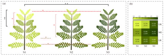
Figure 6. Differences in the vertical distribution of Cephalotaxus hainanensis canopies under different nitrogen application levels. (a) Visualization of the vertical canopy distribution of C. hainanensis under different nitrogen application levels. (b) Predicted nitrogen content of C. hainanensis leaves at different vertical positions under different nitrogen application levels. Note: Values are presented as mean ± standard error (mg·g⁻¹). Statistical significance was determined using one-way analysis of variance (ANOVA) followed by the least significant difference (LSD) test, with significance levels indicated as follows: p < 0.05 (*) and p < 0.01 (**). The color of the asterisks denotes the type of comparison: black asterisks indicate differences at the whole-plant level, whereas red asterisks indicate differences among nitrogen application levels or among plant parts. Nitrogen application levels include N1, N2, and N3, corresponding to 0, 5, and 10 g·plant⁻¹·month⁻¹, respectively. UR, ME, and LR represent the upper, middle, and lower canopy positions, respectively.

Further analysis revealed that nitrogen application level had a significant effect on the vertical distribution pattern of LNC. Across all nitrogen levels, the middle layer consistently exhibited the highest LNC. However, the difference in LNC between the upper and lower layers varied across treatments: in N1 and N2, the lower layer exhibited a higher LNC than the upper layer, whereas in N3, this trend was reversed, with the upper layer’s LNC exceeding that of the lower layer. Significance testing indicated that, under the N1 treatment, LNC differed significantly between the upper and middle layers; under N2, a significant difference was observed between the upper and lower layers, though not between either and the middle layer—likely due to higher data dispersion in the middle layer under this treatment (Figure 6b). No statistically significant differences were detected among canopy layers under the remaining nitrogen treatments.

To further examine the effects of nitrogen treatments in different layers of the plant canopy, a comprehensive comparison was performed. The results showed that LNC under the N1 treatment was consistently lower than that under other treatments across all canopy layers. Specifically, in the upper layer, LNC under N1 was significantly lower than under N3. In the lower layer, LNC under N1 was significantly lower than under both N2 and N3. In the middle layer, no significant differences were found among the treatments. The ranking of LNC across nitrogen levels varied by canopy layers: for the upper and middle layers, the order was N3 > N2 > N1, while for the lower layer, it was N2 > N3 > N1.

3.4. Growth Status of C. hainanensis Under Different Nitrogen Application Levels

Under the N1 and N2 treatments, ground diameter, plant height, and crown diameter of C. hainanensis seedlings exhibited a consistent increasing trend over time. In contrast, under the N3 treatment, both crown diameter and plant height showed a decline in the October 2022 survey. This decrease was primarily attributable to partial seedling mortality and the removal of individuals due to destructive sampling.

At the initial survey, seedling growth status was generally comparable among all nitrogen treatments. As the experiment progressed, seedlings under the N2 treatment exhibited the most favorable overall growth performance, followed by those under N1. Notably, during the October 2022 survey, larger differences in growth metrics were observed between the N2 treatment and the other treatments, although these differences were not statistically significant. By the final survey in May 2023, the growth differences between the N2 and N1 treatments had diminished; nevertheless, seedlings receiving N2 continued to demonstrate superior growth performance compared with those under N1 (Figure 7).

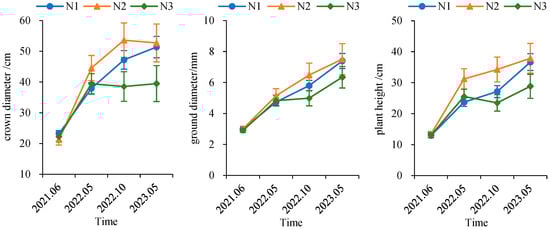
Figure 7. Temporal dynamics of seedling growth in Cephalotaxus hainanensis.

4. Discussion

4.1. Feature Variable Selection

Based on a comprehensive screening using five correlation analysis methods, nine high-frequency variables that were selected by at least three methods were identified. According to their color attributes and construction approaches, these variables can be systematically categorized into three groups. The first category comprises single-channel variables (S, V, L, and b), which exhibited significant differences among all nitrogen treatments (Figure 5), indicating that individual color dimensions possess strong discriminative ability for detecting changes in nitrogen levels. The second category includes composite variables derived from the G and B channels (GMB, GB, and ExB). Among them, GMB was selected by all five methods, suggesting a highly stable and reliable correlation with LNC, and further emphasizing the importance of combining the G and B channels in nitrogen monitoring. The third group comprises normalized color variables (r and DGBVI), both of which effectively reduced environmental interference through normalization and were jointly selected by four methods, demonstrating strong generalizability and practicality in LNC prediction. In summary, this set of high-frequency variables—covering diverse color construction approaches—provides a robust feature foundation for color-based inversion of leaf nitrogen concentration.

It is worth noting that the key variables identified in this study are highly consistent with those reported in previous studies, further confirming their reliability and general applicability. Kawashima and Nakatani [27] reported that r, GMB, and DGBVI are important color indices that are strongly correlated with chlorophyll content. Li et al. [40] further confirmed the significance of GMB in nitrogen response, supporting its suitability for vegetation nitrogen monitoring. Moreover, Agarwal and Dutta Gupta [47] identified r, GMB, DGBVI, and L* as key features in their selection of chlorophyll-related color variables for spinach, which overlaps substantially with the variables identified in the present study. The consistency across multiple studies reinforces the crucial role of these color parameters in plant nitrogen monitoring and demonstrates the effectiveness of the variable selection strategy adopted in this study, as well as its potential applicability across species.

In terms of model performance, the variables selected by the Pearson and Spearman correlation methods exhibited superior predictive accuracy and generalization capability in the SVR model, whereas those obtained by the DC, HSIC, and CE methods showed comparatively weaker generalization. This performance discrepancy may be attributed to the proportion of high-frequency variables retained by each method—Pearson and Spearman preserved a substantially higher proportion than DC, HSIC, and CE—further suggesting that the nine high-frequency variables identified in this study have stable and reliable correlations with LNC.

4.2. Canopy Color Variations

4.2.1. Differences in Canopy Color Characteristics Under Different Nitrogen Levels

Soil nitrogen content is a key environmental factor regulating LNC accumulation in plants [15]. The results of this study showed that LNC progressively increased with higher nitrogen application levels, indicating that the soil nitrogen supply plays a significant role in controlling leaf nitrogen accumulation.

Leaf nitrogen primarily consists of photosynthetic and non-photosynthetic nitrogen components [48], among which photosynthetic nitrogen is closely associated with pigment composition and leaf color characteristics. Therefore, changes in leaf color can serve as an effective indicator of the plant’s nitrogen status [7]. Based on the RGB, HSV, and CIELAB color spaces, this study systematically analyzed the response patterns of different color components to nitrogen application levels. The results revealed that, except for the H component, which exhibited the opposite trend, the variations in other color components were generally consistent with the changes in LNC. Significant differences were observed between N4 and N1 treatments in all color components except for B, suggesting that color parameters across multiple color spaces are effective indicators of nitrogen stress. Furthermore, from the perspective of high-frequency variable screening, single-channel color variables such as S, V, L*, and b* were identified as high-frequency variables, all showing significant differences between N4 and N1 treatments. This finding further verifies the strong correlations between these variables and LNC, highlighting their reliability and potential applicability for leaf nitrogen inversion.

C. hainanensis, as a coniferous species, possesses a relatively high leaf mass per unit area, which results in a greater proportion of total leaf nitrogen being allocated to non-photosynthetic proteins and amino acids, while the investment in photosynthetic nitrogen is comparatively lower [47,49]. This physiological characteristic may reduce the sensitivity of leaf color to nitrogen variation. Consistent with this interpretation, significant color differences were only observed between the N4 and N1 treatments, whereas the intermediate nitrogen treatments did not exhibit consistent or statistically significant color variations.

Although total nitrogen does not reflect the detailed allocation of nitrogen among different biochemical components, it remains a practical and informative indicator of plant nutritional status, particularly under constrained sensing conditions such as RGB image acquisition.

4.2.2. Vertical Heterogeneity of Canopy Color and LNC

According to the leaf economics spectrum, plants tend to allocate more nitrogen to upper canopy leaves to enhance their photosynthetic capacity, thereby promoting the accumulation of growth-related metabolites [13]. This nitrogen allocation strategy leads to pronounced spatial heterogeneity of nitrogen distribution within the canopy, which in turn results in spatial differentiation of color characteristics. The results of this study confirmed the regularity of the spatial color distribution across the canopy, as significant differences were observed between the upper and lower layers in several color components (Figure 5b).

However, the vertical distribution of LNC in C. hainanensis primarily showed differences between the upper and middle layers (Figure 6a), which was inconsistent with the color distribution pattern. This discrepancy may be attributed to several factors: Figure 5b was derived from multi-period observations, whereas Figure 6a was based on LNC inversion results from the final sampling data; dynamic nitrogen allocation during different growth stages and variations in environmental factors may contribute to the observed differences; and the delayed effect of soil nitrogen supply on leaf nitrogen accumulation may also contribute to the inconsistency between canopy color and LNC vertical distribution. Despite these differences, both results consistently demonstrated the spatial heterogeneity of LNC within the canopy.

4.2.3. Applicability of the Canopy-Averaged Nitrogen Estimation Model

When the established overall nitrogen estimation model was further applied to explore vertical nitrogen distribution, LNC was first predicted separately for different canopy positions and then aggregated to represent whole-plant leaf nitrogen. Under this aggregation-based approach, the correlation between predicted and measured nitrogen declined (R² = 0.41; Figure 4). Importantly, this reduction does not indicate a failure of the overall model; rather, it reflects the limited adaptability of a single canopy-averaged model when applied to vertically heterogeneous leaf positions with distinct structural, optical, and physiological characteristics. As uncertainties from position-specific predictions accumulate during aggregation, the overall predictive strength is inevitably reduced. Nevertheless, the model retains practical value for investigating vertical nitrogen distribution patterns, particularly in situations where direct measurement of LNC at individual canopy positions is not feasible.

4.2.4. Nitrogen Allocation Strategy of C. hainanensis Under Different Nitrogen Levels

Although plants generally exhibit a physiological strategy of preferentially allocating nitrogen to upper canopy leaves [50,51], the observations in this study differed from this pattern. In N1 and N2 treatments, upper canopy leaves exhibited the lowest LNC, whereas the middle layer showed the highest values. This phenomenon is closely related to the tropical characteristics of C. hainanensis, which lacks a distinct seasonal growth cycle. Under N1 and N2 conditions, new leaves continuously emerged at the shoot apex, leading to lower nitrogen content in upper leaves. In contrast, under the N3 treatment, excessive nitrogen application suppressed new leaf formation, resulting in upper canopies dominated by mature leaves with higher LNC values than the lower layers.

Across all nitrogen treatments, the middle layer consistently exhibited the highest LNC, suggesting that these mature leaves dominate the photosynthetic canopy and represent the primary sink for nitrogen allocation. Therefore, this study suggests that C. hainanensis follows a nitrogen allocation strategy that prioritizes mature leaves in the upper canopy rather than allocating nitrogen strictly based on vertical canopy position.

Previous studies have consistently demonstrated that nitrogen deficiency primarily affects the lower canopy leaves, whereas excessive nitrogen supply mainly impacts the upper leaves [52,53]. In the present study, it was observed that the LNC of lower leaves under the N1 treatment (low-nitrogen condition) was significantly lower than that under the N2 and N3 treatments. Conversely, under conditions of nitrogen excess (N3 treatment), overall plant growth was inhibited, and nitrogen distribution among canopy layers tended to become uniform, resulting in no significant differences in LNC among the upper, middle, and lower leaves. Moreover, the middle canopy leaves exhibited relatively low sensitivity to nitrogen variation, showing no significant fluctuation in LNC across different nitrogen treatments.

4.2.5. Implications for Nitrogen Diagnosis Based on Canopy Color Differences

Recent work by Shi et al. (2025) [45] demonstrated that color heterogeneity among leaves is more strongly correlated with LNC than mean color values. In this study, the small sample size motivated the use of a vertical canopy structure approach, which allowed us to explore the spatial heterogeneity of leaf nitrogen and reduce potential misinterpretation of nitrogen limitation. The present study found that color differences between upper and lower canopy layers provide an effective diagnostic signal of plant nitrogen status. A small color difference between canopy layers may indicate either nitrogen deficiency or excess; in such cases, the color characteristics of lower leaves can help distinguish between these conditions. In contrast, pronounced color differentiation typically reflects adequate nitrogen supply.

By integrating these strategies, this study provides a practical and reproducible framework for non-destructive nitrogen estimation in a rare conifer species, offering novel insights into leaf nitrogen allocation patterns and demonstrating methodological approaches that can be applied to other non-agricultural, endangered tree species. However, a limitation of this study is that the use of RGB images restricts the inversion to total nitrogen content and does not allow for the discrimination of nitrogen pools associated with different physiological components. Future studies integrating hyperspectral data or biochemical measurements may enable a more detailed partitioning of leaf nitrogen levels.

5. Conclusions

This study conducted a comprehensive statistical analysis for color features selected by five correlation methods and identified nine color feature variables that were highly correlated with LNC. Among them, GMB emerged as the only variable consistently selected across all five methods, demonstrating strong generality and stability in LNC prediction.

A comprehensive assessment across the RGB, HSV, and CIELAB color spaces indicated that color characteristics effectively captured the variation patterns of plant LNC. Under different nitrogen application levels, significant differences in color variables were primarily observed between the N1 and N4 treatments. Within the canopy, pronounced differentiation occurred between the upper and lower layers. Furthermore, by integrating the Spearman-selected variables into a SVR model, the study achieved accurate quantitative inversion of LNC across canopy layers. The results revealed that the vertical distribution of LNC varied among nitrogen treatments, yet the middle canopy consistently maintained the highest LNC. Lower leaves were the most sensitive to nitrogen deficiency, showing significantly lower LNCs under the N1 treatment, with no significant difference between upper and lower layers under this condition. Under excessive nitrogen supply, vertical LNC differences across the canopy diminished, resulting in a more homogeneous nitrogen distribution.

Overall, the N2 treatment represented the optimal nitrogen nutritional status for C. hainanensis. These findings confirm that color features provide a reliable basis for LNC inversion and highlight the diagnostic importance of vertical LNC distribution in evaluating plant nitrogen status.

References

- Abdelkafi, H.; Nay, B. Natural products from Cephalotaxus sp.: Chemical diversity and synthetic aspects. Nat. Prod. Rep. 2012, 29, 845. [Google Scholar] [CrossRef] [PubMed]
- Yu, M.; Huang, S.; Zhang, Y. Chemical constituents of alkaloids part of Cephalotaxus hainanensis. Chin. Tradit. Herbal Drugs 2019, 50, 1541–1545. [Google Scholar]
- Qi, S.; Dai, Z.; Si, C.; Lin, Y.; Yang, D.; Song, J.; Du, D. Study on population structure and resource value of Cephalotaxus mannii Hook. f., a rare and endangered anti-cancer plant in Hainan. For. Resour. Manag. 2010, 1, 53–58. [Google Scholar]
- Wang, R.; Nong, S.; Peng, W.; Wu, B.; Yang, J.; Liao, L. Tree species composition and interspecific associations of rare and endangered plant Cephalotaxus hainanensis community. Ecol. Environ. Sci. 2023, 32, 1741–1749. [Google Scholar]
- Tang, Z.; Xu, W.; Zhou, G.; Bai, Y.; Li, J.; Tang, X.; Chen, D.; Liu, Q.; Ma, W.; Xiong, G.; et al. Patterns of plant carbon, nitrogen, and phosphorus concentration in relation to productivity in China’s terrestrial ecosystems. Proc. Natl. Acad. Sci. USA 2018, 115, 4033–4038. [Google Scholar] [CrossRef]
- Shi, Z.; Tang, J.; Cheng, R.; Luo, D.; Liu, S. A review of nitrogen allocation in leaves and factors in its effects. Acta Ecol. Sin. 2015, 35, 5909–5919. [Google Scholar]
- Evans, J.R.; Clarke, V.C. The nitrogen cost of photosynthesis. J. Exp. Bot. 2019, 70, 7–15. [Google Scholar] [CrossRef]
- Guan, C.; Zhang, D.; Chu, C. Interplay of light and nitrogen for plant growth and development. Crop J. 2025, 13, 641–655. [Google Scholar] [CrossRef]
- Wen, B.; Li, C.; Fu, X.; Li, D.; Li, L.; Chen, X.; Wu, H.; Cui, X.; Zhang, X.; Shen, H.; et al. Effects of nitrate deficiency on nitrate assimilation and chlorophyll synthesis of detached apple leaves. Plant Physiol. Biochem. 2019, 142, 363–371. [Google Scholar] [CrossRef]
- Peng, S.; Bao, N.; Gu, N.; Qian, H.; Han, Z.; Zhou, B.; Chang, L. Enhanced assessment of chlorophyll-a and total nitrogen dynamics using unmanned aerial vehicle-based model and hyperspectral imagery in coastal wetland water. Environ. Technol. Innov. 2025, 40, 104521. [Google Scholar] [CrossRef]
- Sun, X.; Zhang, B.; Zhang, Z.; Jing, C.; Gu, L.; Zhen, W.; Gu, X. Coupling decision of water and nitrogen application in winter wheat via UAV hyperspectral imaging. Field Crops Res. 2025, 334, 110159. [Google Scholar] [CrossRef]
- Li, H.; Zhao, C.; Huang, W.; Yang, G. Non-uniform vertical nitrogen distribution within plant canopy and its estimation by remote sensing: A review. Field Crops Res. 2013, 142, 75–84. [Google Scholar] [CrossRef]
- Zhao, C.; Li, H.; Li, P.; Yang, G.; Gu, X.; Lan, Y. Effect of vertical distribution of crop structure and biochemical parameters of winter wheat on canopy reflectance characteristics and spectral indices. IEEE Trans. Geosci. Remote Sens. 2017, 55, 236–247. [Google Scholar] [CrossRef]
- Hikosaka, K.; Anten, N.P.R.; Borjigidai, A.; Kamiyama, C.; Sakai, H.; Hasegawa, T.; Oikaw, S.; Iio, A.; Watanabe, M.; Koike, T.; et al. A meta-analysis of leaf nitrogen distribution within plant canopies. Ann. Bot. 2016, 118, 239–247. [Google Scholar] [CrossRef]
- Walters, M.B.; Gerlach, J.P. Intraspecific growth and functional leaf trait responses to natural soil resource gradients for conifer species with contrasting leaf habit. Tree Physiol. 2013, 33, 297–310. [Google Scholar] [CrossRef]
- He, J.; Zhang, X.; Guo, W.; Pan, Y.; Yao, X.; Cheng, T.; Zhu, Y.; Cao, W.; Tian, Y. Estimation of vertical leaf nitrogen distribution within a rice canopy based on hyperspectral data. Front. Plant Sci. 2020, 10, 1802. [Google Scholar] [CrossRef]
- Qiu, Z.; Ma, F.; Li, Z.; Xu, X.; Ge, H.; Du, C. Estimation of nitrogen nutrition index in rice from UAV RGB images coupled with machine learning algorithms. Comput. Electron. Agric. 2021, 189, 106421. [Google Scholar] [CrossRef]
- Hamuda, E.; Glavin, M.; Jones, E. A survey of image processing techniques for plant extraction and segmentation in the field. Comput. Electron. Agric. 2016, 125, 184–199. [Google Scholar] [CrossRef]
- Lee, K.-J.; Lee, B.-W. Estimation of rice growth and nitrogen nutrition status using color digital camera image analysis. Eur. J. Agron. 2013, 48, 57–65. [Google Scholar] [CrossRef]
- Li, R.; Wang, D.; Zhu, B.; Liu, T.; Sun, C.; Zhang, Z. Estimation of nitrogen content in wheat using indices derived from RGB and thermal infrared imaging. Field Crops Res. 2022, 289, 108735. [Google Scholar] [CrossRef]
- Wang, Y.; Wang, D.; Zhang, G.; Wang, J. Estimating nitrogen status of rice using the image segmentation of G-R thresholding method. Field Crops Res. 2013, 149, 33–39. [Google Scholar] [CrossRef]
- Xu, Y.; Wang, X.; Sun, H.; Wang, H.; Zhan, Y. Study of monitoring maize leaf nutrition based on image processing and spectral analysis. In Proceedings of the 2010 World Automation Congress, Kobe, Japan, 19–23 September 2010; pp. 465–468. [Google Scholar]
- Li, S.; Yuan, F.; Ata-UI-Karim, S.T.; Zheng, H.; Cheng, T.; Liu, X.; Tian, Y.; Zhu, Y.; Cao, W.; Cao, Q. Combining color indices and textures of UAV-based digital imagery for rice LAI estimation. Remote Sens. 2019, 11, 1763. [Google Scholar] [CrossRef]
- Woebbecke, D.M.; Meyer, G.E.; Von Bargen, K.; Mortensen, D.A. Color indices for weed identification under various soil, residue, and lighting conditions. Trans. ASAE 1995, 38, 259–269. [Google Scholar] [CrossRef]
- Sulik, J.J.; Long, D.S. Spectral considerations for modeling yield of canola. Remote Sens. Environ. 2016, 184, 161–174. [Google Scholar] [CrossRef]
- Gitelson, A.A.; Kaufman, Y.J.; Stark, R.; Rundquist, D. Novel algorithms for remote estimation of vegetation fraction. Remote Sens. Environ. 2002, 80, 76–87. [Google Scholar] [CrossRef]
- Kawashima, S.; Nakatani, M. An algorithm for estimating chlorophyll content in leaves using a video camera. Ann. Bot. 1998, 81, 49–54. [Google Scholar] [CrossRef]
- Louhaichi, M.; Borman, M.M.; Johnson, D.E. Spatially located platform and aerial photography for documentation of grazing impacts on Wheat. Geocarto Int. 2001, 16, 65–70. [Google Scholar] [CrossRef]
- Bendig, J.; Yu, K.; Aasen, H.; Bolten, A.; Bennertz, S.; Broscheit, J.; Gnyp, M.L.; Bareth, G. Combining UAV-based plant height from crop surface models, visible, and near infrared vegetation indices for biomass monitoring in barley. Int. J. Appl. Earth Obs. Geoinf. 2015, 39, 79–87. [Google Scholar] [CrossRef]
- Guo, Y.; Xiao, Y.; Li, M.; Hao, F.; Zhang, X.; Sun, H.; Beurs, K.; Fu, Y.H.; He, Y. Identifying crop phenology using maize height constructed from multi-sources images. Int. J. Appl. Earth Obs. Geoinf. 2022, 115, 103121. [Google Scholar] [CrossRef]
- Woebbecke, D.M.; Meyer, G.E.; Von Bargen, K.; Mortensen, D.A. Plant species identification, size, and enumeration using machine vision techniques on near-binary images. In Proceedings of the Applications in Optical Science and Engineering, Boston, MA, USA, 16 November 1992; DeShazer, J.A., Meyer, G.E., Eds.; SPIE: Bellingham, WA, USA, 1993; pp. 208–219. [Google Scholar] [CrossRef]
- Hague, T.; Tillett, N.D.; Wheeler, H. Automated crop and weed monitoring in widely spaced cereals. Precis. Agric. 2006, 7, 21–32. [Google Scholar] [CrossRef]
- Meyer, G.E.; Neto, J.C. Verification of color vegetation indices for automated crop imaging applications. Comput. Electron. Agric. 2008, 63, 282–293. [Google Scholar] [CrossRef]
- Qi, J.; Chehbouni, A.; Huete, A.R.; Kerr, Y.H.; Sorooshian, S. A Modified soil adjusted vegetation index. Remote Sens. Environ. 1994, 48, 119–126. [Google Scholar] [CrossRef]
- Meyer, G.E.; Neto, J.C.; Jones, D.D.; Hindman, T.W. Intensified fuzzy clusters for classifying plant, soil, and residue regions of interest from color images. Comput. Electron. Agric. 2004, 42, 161–180. [Google Scholar] [CrossRef]
- Kataoka, T.; Kaneko, T.; Okamoto, H.; Hata, S. Crop growth estimation system using machine vision. In Proceedings of the 2003 IEEE/ASME International Conference on Advanced Intelligent Mechatronics (AIM 2003), Kobe, Japan, 20–24 July 2003; IEEE: New York, NY, USA, 2003; pp. b1079–b1083. [Google Scholar] [CrossRef]
- Guijarro, M.; Pajares, G.; Riomoros, I.; Herrera, P.J.; Burgos-Artizzu, X.P.; Ribeiro, A. Automatic segmentation of relevant textures in agricultural images. Comput. Electron. Agric. 2011, 75, 75–83. [Google Scholar] [CrossRef]
- Burgos-Artizzu, X.P.; Ribeiro, A.; Guijarro, M.; Pajares, G. Real-time image processing for crop/weed discrimination in maize fields. Comput. Electron. Agric. 2011, 75, 337–346. [Google Scholar] [CrossRef]
- Guerrero, J.M.; Pajares, G.; Montalvo, M.; Romeo, J.; Guijarro, M. Support Vector Machines for crop/weeds identification in maize fields. Expert. Syst. Appl. 2012, 39, 11149–11155. [Google Scholar] [CrossRef]
- Li, D.; Li, C.; Yao, Y.; Li, M.; Liu, L. Modern imaging techniques in plant nutrition analysis: A review. Comput. Electron. Agric. 2020, 174, 105459. [Google Scholar] [CrossRef]
- Saberioon, M.M.; Amin, M.S.M.; Anuar, A.R.; Gholizadeh, A.; Wayayok, A.; Khairunniza-Bejo, S. Assessment of rice leaf chlorophyll content using visible bands at different growth stages at both the leaf and canopy scale. Int. J. Appl. Earth Obs. Geoinf. 2014, 32, 35–45. [Google Scholar] [CrossRef]
- Jiang, J.; Cai, W.; Zheng, H.; Cheng, T.; Tian, Y.; Zhu, Y.; Ehsani, R.; Hu, Y.; Niu, Q.; Gui, L.; et al. Using digital cameras on an unmanned aerial vehicle to derive optimum color vegetation indices for leaf nitrogen concentration monitoring in winter wheat. Remote Sens. 2019, 11, 2667. [Google Scholar] [CrossRef]
- Kazmi, W.; Garcia-Ruiz, F.J.; Nielsen, J.; Rasmussen, J.; Andersen, H.J. Detecting creeping thistle in sugar beet fields using vegetation indices. Comput. Electron. Agric. 2015, 112, 10–19. [Google Scholar] [CrossRef]
- Li, J.; Zhang, F.; Qian, X.; Zhu, Y.; Shen, G. Quantification of rice canopy nitrogen balance index with digital imagery from unmanned aerial vehicle. Remote Sens. Lett. 2015, 6, 183–189. [Google Scholar] [CrossRef]
- Shi, M.; Wang, T.; Lin, L.; Li, Q.; Chen, Z.; Chen, X.; Wang, P.; Wang, X. Regression-based leaf nitrogen concentration estimation of young Cephalotaxus hainanensis in small and imbalanced samples. Smart Agric. Technol. 2025, 12, 101195. [Google Scholar] [CrossRef]
- Chen, Z.; Wang, X.; Sun, S. Estimating the total nitrogen content of Aquilaria sinensis leaves based on a hybrid feature selection algorithm and image data from a modified digital camera. Biosyst. Eng. 2022, 213, 89–104. [Google Scholar] [CrossRef]
- Agarwal, A.; Dutta Gupta, S. Assessment of spinach seedling health status and chlorophyll content by multivariate data analysis and multiple linear regression of leaf image features. Comput. Electron. Agric. 2018, 152, 281–289. [Google Scholar] [CrossRef]
- Li, D.; Chen, J.M.; Yan, Y.; Zheng, H.; Yao, X.; Zhu, Y.; Cao, W.; Cheng, T. Estimating leaf nitrogen content by coupling a nitrogen allocation model with canopy reflectance. Remote Sens. Environ. 2022, 283, 113314. [Google Scholar] [CrossRef]
- Luo, X.; Keenan, T.F.; Chen, J.M.; Croft, H.; Colin Prentice, I.; Smith, N.J.; Walker, A.P.; Wang, H.; Wang, R.; Xu, C.; et al. Global variation in the fraction of leaf nitrogen allocated to photosynthesis. Nat. Commun. 2021, 12, 4866. [Google Scholar] [CrossRef] [PubMed]
- Li, L.; Jákli, B.; Lu, P.; Croft, H.; Prentice, I.C.; Smith, N.G.; Walker, A.P.; Wang, H.; Wang, R.; Xu, C.; et al. Assessing leaf nitrogen concentration of winter oilseed rape with canopy hyperspectral technique considering a non-uniform vertical nitrogen distribution. Ind. Crops Prod. 2018, 116, 1–14. [Google Scholar] [CrossRef]
- Xiao, X.; Zang, H.; Liu, Y.; Zhang, Z.; Liu, Y.; Ejaz, I.; Du, C.; Wang, Z.; Sun, Z.; Zhang, Y. Promoting winter wheat sustainable intensification by higher nitrogen distribution in top second to fourth leaves under water-restricted condition in North China Plain. Agric. Water Manag. 2023, 289, 108551. [Google Scholar] [CrossRef]
- Zhao, X.; Liu, Z.; Jin, G. Effects of nitrogen addition and leaf age on needle traits and the relationships among traits in Pinus koraiensis. Environ. Exp. Bot. 2024, 223, 105795. [Google Scholar] [CrossRef]
- Huang, W.; Yang, Q.; Pu, R.; Yang, S. Estimation of nitrogen vertical distribution by bi-directional canopy reflectance in winter wheat. Sensors 2014, 14, 20347–20359. [Google Scholar] [CrossRef]
Disclaimer/Publisher’s Note: The statements, opinions and data contained in all publications are solely those of the individual author(s) and contributor(s) and not of MDPI and/or the editor(s). MDPI and/or the editor(s) disclaim responsibility for any injury to people or property resulting from any ideas, methods, instructions or products referred to in the content. |
© 2026 by the authors. Licensee MDPI, Basel, Switzerland. This article is an open access article distributed under the terms and conditions of the Creative Commons Attribution (CC BY) license.