You are currently viewing a new version of our website. To view the old version click .
Forests
  • Article
  • Open Access

11 November 2025

Urban Greening Strategies and Ecosystem Services: The Differential Impact of Street-Level Greening Structures on Housing Prices

,
,
,
,
,
,
,
and
1
School of Architecture, Tianjin Chengjian University, Tianjin 300380, China
2
International Centre for Bamboo and Rattan, Beijing 100102, China
3
Key Laboratory of National Forestry and Grassland Administration, Beijing for Bamboo & Rattan Science and Technology, Beijing 100102, China
4
International School of Engineering, Tianjin Chengjian University, Tianjin 300380, China
This article belongs to the Special Issue Urban Forests and Greening for Sustainable Cities

Abstract

Street greening is widely recognized as influencing resident well-being and housing prices, and street-view imagery provides a fine-grained data source for quantifying urban microenvironments. However, existing research predominantly relies on single indicators such as the Green View Index (GVI) and overall green coverage/volume lacking a systematic analysis of how the hierarchical structure of trees, shrubs, and grass relates to housing prices. This study examines the high-density block context of Tianjin’s six urban districts. Using the Street Greening Space Structure (SGSS) dataset to construct greening structure configurations, we integrate housing-price data, neighborhood attributes, and 13,280 street-view images from the study area. We quantify how “visibility and hierarchical ratios” are capitalized on in the housing market and identify auditable threshold ranges and contextual gating. We propose an urban–forest structural system centered on visibility and hierarchical ratios that links street-level observability to ecosystem services. Employing an integrated framework combining Geographical-XGBoost (G-XGBoost) and SHapley Additive exPlanations (SHAP), we move beyond average effects to reveal structural detail and contextual heterogeneity in capitalization. Our findings indicate that tree visibility G_TVI is the most robust and readily capitalized price signal: when G_TVI increases from approximately 0.06 to 0.12–0.16, housing prices rise by about 8%–10%. Hierarchical structure is crucial: balanced tree–shrub ratios and moderate shrub–grass ratios translate “visible green” into functional green. Capitalization effects are environmentally conditioned—more pronounced along corridors with high centrality and accessibility—and are likewise common in dense East Asian metropolises (e.g., Beijing, Shanghai, Seoul, and Tokyo) and rapidly motorizing cities (e.g., Bangkok and Jakarta). These patterns suggest parametric prescriptions that prioritize canopy-corridor continuity and keep ratios within actionable threshold bands. We translate these findings into urban greening strategies that prioritize canopy continuity, under-canopy permeability, and maintainability, providing sustainability-oriented, parameterized guidance for converting urban greening structure into ecological capital for sustainable cities.

1. Introduction

In recent years, urban housing prices have been widely used to characterize residential preferences and spatial quality [,,]. Against the backdrop of concurrent rapid greenfield development and stock renewal, supply–demand imbalances alone are insufficient to explain the spatial heterogeneity of housing prices [,]. Urban expansion not only intensifies supply–demand conflicts but also raises expectations for residential environmental quality. Beyond supply and demand, microenvironmental quality is emerging as a critical dimension shaping heterogeneous residential pricing []. A large body of research shows that street greening is positively associated with welfare indicators such as thermal environment, air quality, walkability, and resident health and satisfaction [,]; from an economic perspective, these perceived and functional improvements translate into higher willingness to pay and are capitalized into housing prices [,,], with effects further amplified by layout and structural optimization. Although these associations have been repeatedly documented, existing evidence primarily focuses on aggregate green coverage or a single Green View Index (GVI), with insufficient attention to the hierarchical structure and proportion of street greenery [,]. Accordingly, clarifying how the hierarchical structure and proportional composition of street greenery relate to housing prices has become a topic requiring systematic examination. Focusing on the secondary apartment listing market in Tianjin’s six urban districts, this study systematically investigates how street greenery is capitalized in the housing market from the structural perspective of “visibility and hierarchical proportion”.
Housing prices are typically determined by multiple factors, including structural characteristics, locational conditions, and neighborhood attributes [,]. In recent years, an increasing number of studies have incorporated street greening into heterogeneous pricing frameworks, generally finding that higher greening levels are associated with stronger capitalization []. Existing evidence primarily relies on quantitative indicators such as canopy cover, vegetation indices, or tree counts [,], as well as visible green metrics derived from street-view imagery and remote sensing, revealing the association between “visible greenery” and market pricing []. However, these metrics predominantly focus on aggregate quantities, with insufficient attention to the hierarchical structure and proportional composition of trees, shrubs, and grass. Moreover, their estimated significance varies across spatial and temporal contexts, suggesting that aggregate metrics alone cannot explain price differentials [] nor clarify under which structural configurations and contexts green spaces are more fully capitalized [,]. Ecological and landscape studies further indicate that continuous tree canopies significantly reduce pedestrian-side mean radiant temperature and alleviate heat stress through shading and evapotranspiration; moderate shrub layers enhance near-ground landscape hierarchy and perceived safety, whereas overly dense shrubbery increases aerodynamic drag, weakens ventilation and under-canopy permeability, and poses visibility and safety risks; grass layers exhibit relatively limited direct cooling effects but enhance infiltration and retention, improving site accessibility and recreational value [,,]. Thus, street-greenery structures comprehensively improve microclimate, visual landscapes, and social-interaction environments, influencing residents’ perceptions and housing prices [,,]. Therefore, systematically examining how street greenery is capitalized in the housing market from a structural and proportional perspective is essential for refining the evidence base and informing planning practices. To facilitate systematic comparison and positioning relative to the closest prior studies, Table 1 summarizes the differences in indicators, models, and key findings between this research and related work.
To identify the market role of street-greenery structure and composition, it is essential to establish a quantitative framework that can stably characterize visibility and hierarchical structure at the urban scale []. Traditional questionnaires and field surveys are costly and struggle to achieve citywide coverage []. In recent years, the large-scale availability of Street View imagery (SVI), combined with mature machine learning and deep-learning techniques, has markedly enhanced spatiotemporal scalability []. The most common approach is to compute the Green View Index (GVI) to capture visible greenery from the pedestrian perspective. Meanwhile, computer-vision methods for canopy segmentation in Street View imagery have substantially improved the accuracy and scalability of such metrics [,,]. Street-view big data has also spurred specialized datasets: (i) large-scale GVI datasets that validate street-level visible greenery against NDVI [,]; and (ii) deep-learning semantic-segmentation datasets for urban vegetation (e.g., trees and grass) used for greening monitoring []. At the metric level, tree visibility can serve as a proxy for shade–ventilation compatibility, helping to consistently demonstrate how ecosystem services are recognized by the housing market and reflected in prices [,]. The emergence of finely annotated street-greening datasets in recent years enables hierarchical identification and structured quantification. For example, the Street Greening Space Structure (SGSS) dataset developed by Zhang et al. [] subdivides vegetation into trees, shrubs, and grass with pixel-level annotations. This fills a gap in street-scale greening structure data, provides high-quality support for subsequent analyses of hierarchical street-greening configurations (tree–shrub–grass combinations), and establishes both methodological and data foundations for investigating how such structures are capitalized in the housing market.
In terms of research methodology, the Hedonic Price Model (HPM) is widely employed to infer residents’ willingness to pay for different housing attributes. This approach treats real-estate prices as a function of the combined value of quantifiable attributes and decomposes them into structural, neighborhood, and locational components []. To more comprehensively assess the influence of urban environmental factors on housing prices, researchers have begun incorporating street-level variables into HPMs for integrated analysis. For example, McCord [] reports a significant price premium associated with blue–green spaces, while Ye [] finds that street greening and accessibility are positively correlated with housing prices, with street greening standing out among environmental covariates. Traditional empirical studies predominantly employ OLS estimation for its simplicity and interpretability, yet its linearity assumptions limit the modeling of nonlinear relationships and variable interactions []. To capture spatial variation, some studies adopt GWR to reveal spatially varying coefficients []; however, its performance is sensitive to bandwidth and kernel choices and it struggles to accommodate complex nonlinear structures within a unified framework. This need is particularly pronounced for microclimate-related benefits: shading and ventilation effects are jointly modulated by road orientation, street-canyon (street-valley) morphology, accessibility, and centrality, exhibiting location-dependent nonlinear gating []. Therefore, a unified framework is required to capture nonlinearity and spatial non-stationarity simultaneously, avoiding the dilution of mechanism-specific differences into a single averaged effect. Consistent with this direction, recent work combines machine learning with spatial modeling (e.g., Geo-RF and Geo-XGBoost) to overcome linear-model limitations and more effectively capture nonlinear interactions, higher-order effects, and heterogeneous distributions [,]. Concurrently, GeoShapley equips machine learning models with interpretability tools for quantifying geographic influence []. Building on this foundation, this paper unifies model learning, result interpretation, and scenario diagnosis within the same framework, reducing biases arising from tensions between global and local effects while explicitly translating microclimate-related structural thresholds and location gating into actionable metrics.
In summary, this study leverages the Street Greening Space Structure (SGSS) dataset and deep learning to precisely extract hierarchical structural features of street greenery. Within a unified framework that integrates Geographical-XGBoost v1.0.9(G-XGBoost) with SHapley Additive exPlanations v0.48(SHAP), we construct a quantitative indicator system for street greenery visibility and hierarchical ratios and explicitly link it to housing-price capitalization. In doing so, we address gaps in the literature on micro-scale green structure and housing prices, specifically the absence of structure sensitive indicators and insufficient threshold analysis, and we systematically examine how visibility and hierarchical ratios are capitalized by the market. We also propose a city scale framework for analyzing the relationship between green structure and housing prices, providing implementable threshold bands and priorities for street segment micro upgrades aimed at enhancing thermal comfort and safety. By moving beyond quantity only metrics (for example, NDVI and GVI) and systematically introducing the hierarchical analysis of trees, shrubs, and grass, the study offers a more comprehensive perspective for housing-price research. Based on urban scale empirical evidence, this study identifies actionable structural signals and contextual variation. It provides executable quantitative foundations for street segment micro renewal and valuation practice, supporting thermal comfort and public health, sustainable mobility, climate adaptation and resilience, and equitable access to green space. This enables residents to enjoy more comfortable street experiences in daily commutes and leisure activities, while robustly translating the ecological and social benefits of urban–forest structure into spatial quality and market value. Building on these contributions, the paper focuses on the following urban scale objectives:
(O1)
Identify and quantify the relationships between multi level visibility and proportional composition and housing prices, clarifying the direction and magnitude of capitalization after controlling for structural, neighborhood, and locational attributes.
(O2)
Reveal nonlinear thresholds, scenario dependence, and spatial heterogeneity in the relationship between greening structure and prices.
(O3)
Translate threshold ranges and contextual conditions of street-greening structure into implementation guidelines for street segment micro upgrades.
Table 1. Comparative review of related studies on street-view vegetation metrics, models, and findings.
StudyAreaGreen MetricModel
Zhang []Beijing (parcel/segment)GVI from SVI (single number)Hedonic OLS (global)
What’s new: Move from single GVI to a visibility plus hierarchy framework; use explicit canopy-understory ratios; learn thresholds and spatial nonstationarity within one model.
Wu []Multi-city (CN)Visual contact / ML features from SVIML + Hedonic (integrated)
What’s new: Define actionable structure ratios (G_TBR, G_BGR) and quantify effective bands.
Su []Shanghai (street)Daily accessed greenery (exposure)Hedonic (linear regression)
What’s new: Distinguish canopy from near-ground layering and show context-gated returns.
Lin []NYC (building)Tree abundance / management proxiesSpatial hedonic (SAR/SEM)
What’s new: Provide visibility indices and ratio structure; identify nonlinear thresholds using local SHAP maps.
Xu []Chinese cityML greenness + urban visual intelligenceRandom Forest (global) + AHP
What’s new: Apply Geographical-XGBoost to learn nonlinearity and spatial nonstationarity with interpretable SHAP.
Donovan []Portland (US)Street trees (counts/presence)Hedonic (price) + TOM model
What’s new: Translate results into SVI visibility bands and ratio thresholds for segment-level upgrades.
Sander []Twin Cities (US)Tree canopy cover (TCC)Hedonic (SAR error)
What’s new: Reveal plateaus and penalties, and show how near-ground layering modifies gains.

2. Study Area and Data

2.1. Research Framework

Figure 1 outlines the workflow of this study, including data collection, data processing, housing-price modeling, and analysis. First, we assembled a multi-source dataset comprising housing-price information, street-view imagery, and points of interest (POIs). Second, we filtered and spatially overlaid the housing-price and POI data in ArcMap. Using Baidu Maps street-view imagery, we applied image segmentation with the DeepLabv3+ (https://github.com/VainF/DeepLabV3Plus-Pytorch, accessed on 26 May 2025) model (convolutional neural network) to extract street-level greenery structure features. These features were then incorporated into the housing-price modeling. Finally, we used OLS as the baseline housing-price model and conducted Moran’s I and Lagrange multiplier tests on the OLS residuals to demonstrate spatial autocorrelation and spatial heterogeneity. We then adopted the Geographical-XGBoost v1.0.9 (G-XGBoost) algorithm and used SHAP v0.48 (SHapley Additive exPlanations) for interpretation to explore the spatial relationships between housing prices, greenery structures, and related factors, and to compare the effects and roles of different greenery structures on housing prices.
Figure 1. Study workflow from multi-source data to model interpretation.

2.2. Study Area

This study selects the central urban districts of Tianjin (the six urban districts: Heping, Hexi, Nankai, Hedong, Hebei, and Hongqiao) as the empirical area, as seen in Figure 2. Tianjin is located on the northern North China Plain 116 43 118 04 E , 38 34 40 15 N and serves as a major port city and a municipality directly under the central government in northern China. In 2020, the city’s land area was approximately 11 , 966 km 2 , its permanent resident population was about 13.82 million, and the urbanization rate reached 82.57%. The six urban districts constitute the earliest-developed and most functionally concentrated built-up areas, exhibiting typical old-city characteristics such as high density, mixed-use development, and fine-grained alleyways. In recent years, the rapid expansion of the rail-transit network has created pronounced accessibility and price gradients along its corridors. Climatically, Tianjin has a warm-temperate monsoon climate with high thermal loads in summer; shade from street trees and ventilation corridors are therefore critical for thermal comfort. In terms of street-greening structure, the central urban area commonly features relatively narrow green belts enclosed by street trees and shrubs; traditional historic districts and lane-style neighborhoods tend to have even narrower belts dominated by enclosed trees and shrubs. By contrast, waterfront thoroughfares and major urban arteries more readily form strip-like, continuous layered configurations of trees, shrubs, and grass, supplemented by pocket parks and corner green spaces. These granular differences in strip width, continuity, and layering provide quasi-natural controls for quantifying green structure and comparing its relationship with housing prices. Building on this context, we employ street-view imagery (SVI) alongside housing-price data. By integrating the SGSS dataset with deep-learning semantic segmentation, we extract tree–shrub–grass elements at the street scale and construct greening structure indicators. These indicators allow us to identify scenario-specific variations in the relationship between greening structure and housing prices across the central urban area, thereby providing a robust research framework and data foundation for the subsequent empirical analysis.
Figure 2. Overview of study area for the present study. (a) Tianjin is located in the north of China. (b) Overview of Tianjin. (c) Names of districts in the study area, CBD locations.

2.3. Data

Table 2 summarizes the multi-source datasets used in this study. Second-hand housing listing and transaction data were obtained from Anjuke (https://tj.fang.anjuke.com/ accessed on 26 May 2025), which covers most major Chinese cities and is among the country’s most widely used real-estate platforms. Within the study area, we collected 3180 neighborhood-level public listing records via web scraping, with coverage up to 2024. Variable selection and definitions were based on practical needs while considering data availability and relevant literature [,]. The variables include property type (s_property), building age (s_age), year built (s_yearbuilt), floor area ratio (s_far), green coverage ratio (s_greenrate), building type (s_bldgtype), and property management fee (s_mgmtfee). We then cleaned the raw data by removing missing and duplicate records, standardizing the price unit to RMB yuan per square meter, and conducting basic outlier screening. During preprocessing, the housing-price variable was log-transformed to mitigate skewness for subsequent modeling. Categorical fields—such as property type (e.g., ordinary residence, apartment residence) and building type (e.g., low-rise, mid-rise, and high-rise)—were encoded as dummy variables using one-hot encoding to avoid information loss or model bias stemming from categorical variables. Finally, we used Baidu Maps geocoding services to complete geocoding and coordinate system conversion (standardized to WGS 84), and merged structural attributes with the housing-price dataset. Following the “15-min living circle” principle, we constructed a 1 km buffer centered on each residential community as the spatial analysis unit to represent the range of routine walking accessibility for residents; neighborhood and environmental characteristics were then extracted within this buffer [].
Table 2. Descriptive statistics of all variables (units and coding clarified).
Additionally, neighborhood-attribute data primarily originate from point-of-interest (POI) records on the AutoNavi (AMap) platform. The data come from the 2024 Tianjin POI dataset and were obtained via the AMap API. Based on HPM modeling requirements for neighborhood environments, the original POI categories were mapped by typecode to four groups (Hospital/School/Commercial/Transport), deduplicated, and valid points were retained Table 3. For each residential point, we extracted the shortest network distance to the nearest subway station or bus stop (t_transport), as well as counts of schools (school_n), hospitals (hospital_n), and recreational facilities (recreation_n) within a 500 m radius. These indicators characterize neighborhood accessibility and public-service levels. We also report a consolidated transit-access measure, HubDist, defined as the shortest network distance to the nearest mass-transit node (subway station or bus stop) Table 3. For locational attributes, we introduce the shortest network distance from each residence to the central business district (CBD) as a spatial-centrality indicator. Tianjin’s CBD is defined as the Xiaobailou Commercial District in Heping District, which concentrates financial, commercial, and high-end office functions and represents the city’s primary functional core. The shortest network distance (t_CBD) from each residential point to the CBD was calculated in QGIS 3.34 using the road network from OpenStreetMap (OSM, https://download.geofabrik.de/ accessed on 26 May 2025) via a shortest-path algorithm Figure 3.
Table 3. POI major types and selected Amap (Gaode) subcategories; coverage is computed within each major type.
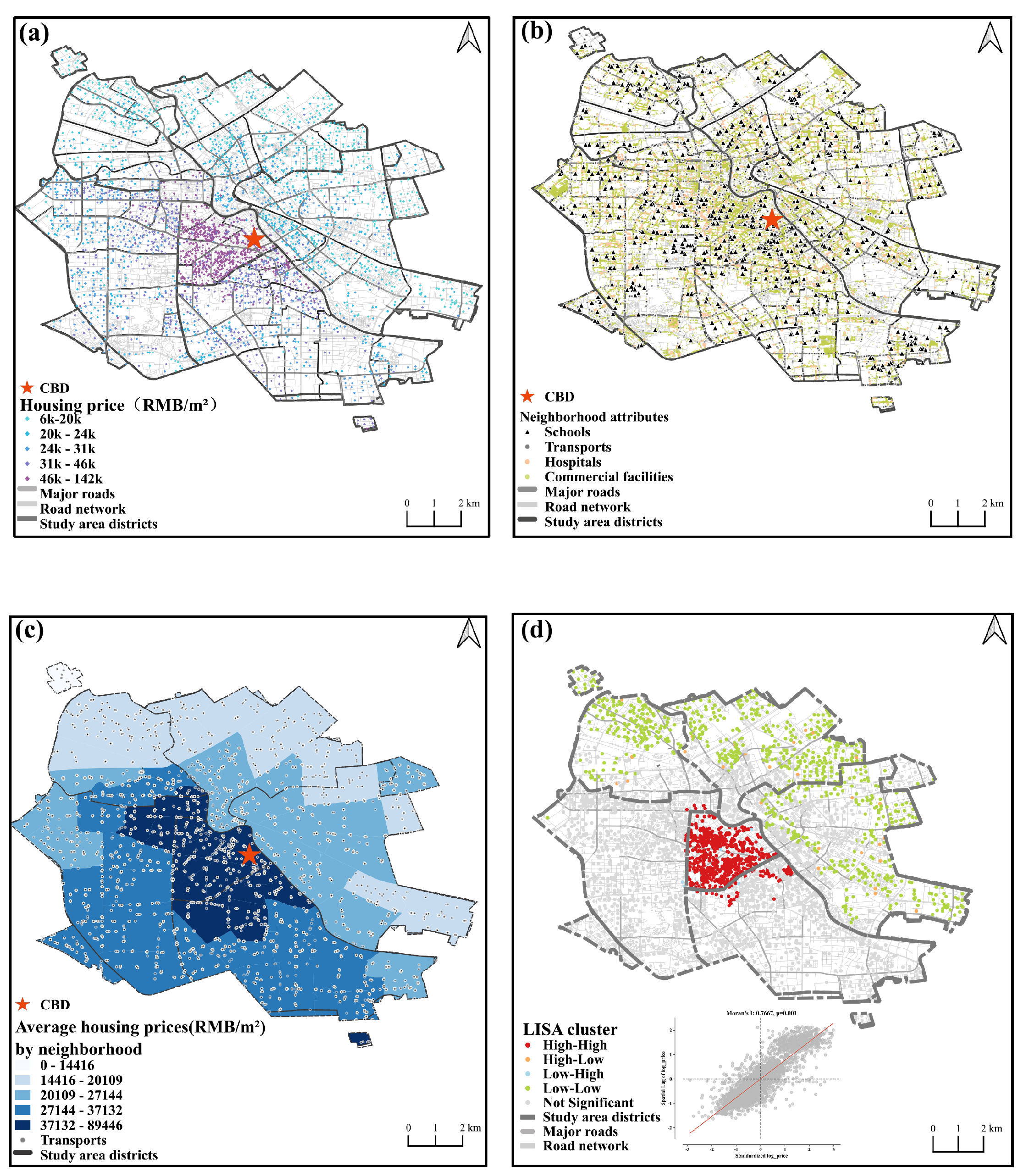
Figure 3. Spatial distribution of (a) residential transaction prices, (b) community attributes (including points of interest for amenities and services, underground stations, employment opportunities, and secondary school distribution), (c) average property prices by street (RMB per square meter), and (d) LISA clustering analysis of logarithmic prices (hotspot distribution).
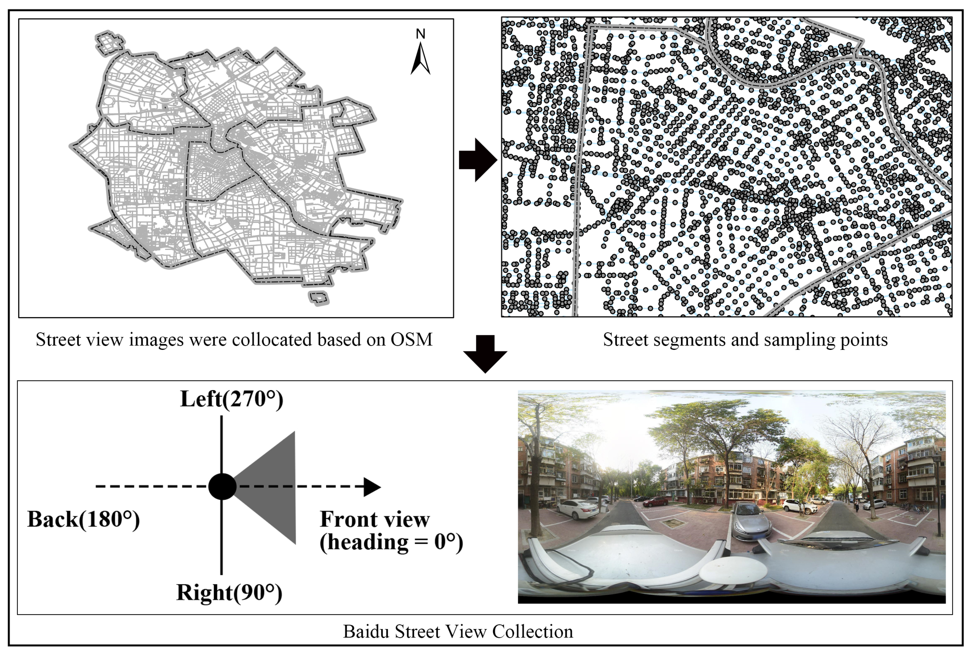
The street-view imagery used in this study was obtained via the Baidu Maps Panorama API v3.0. As a leading map-service provider in China, the platform offers an application programming interface (API) that enables programmatic, batched retrieval of street-view images, as illustrated in Figure 4. We first acquired the road network for the study area (UTM coordinates) using the OSMnx v2.0.6 library in Python 3.8 and placed points at 100 m intervals along road centerlines. Using a KDTree-based nearest neighbor search, we deduplicated points that were closer than 100 m to one another, yielding 16,638 candidate sampling locations. WGS 84 coordinates were converted to Baidu Mercator (BD09MC) via the Baidu geocoding API. For each sampling location, we requested panoramic tiles at four azimuths ( 0 , 90 , 180 , 270 ) with uniform settings (field of view = 90°, pitch = 0°, resolution 2048 × 1024 ) to reduce unilateral occlusion bias. Images were retained only when complete metadata were available, with the target year standardized to 2021; where multiple vintages existed for the same location, the target-year image or the closest available vintage was selected. To minimize the impact of leaf-off conditions on greenery identification, we restricted the growing season to April through October. Scenes under tunnels or overpasses, severely blurred images, and low-light images were excluded, and resolution was standardized to 2048 × 1024 . In total, 13,280 panoramic street-view images were collected.
Figure 4. The process of Baidu 360° panoramic collection.
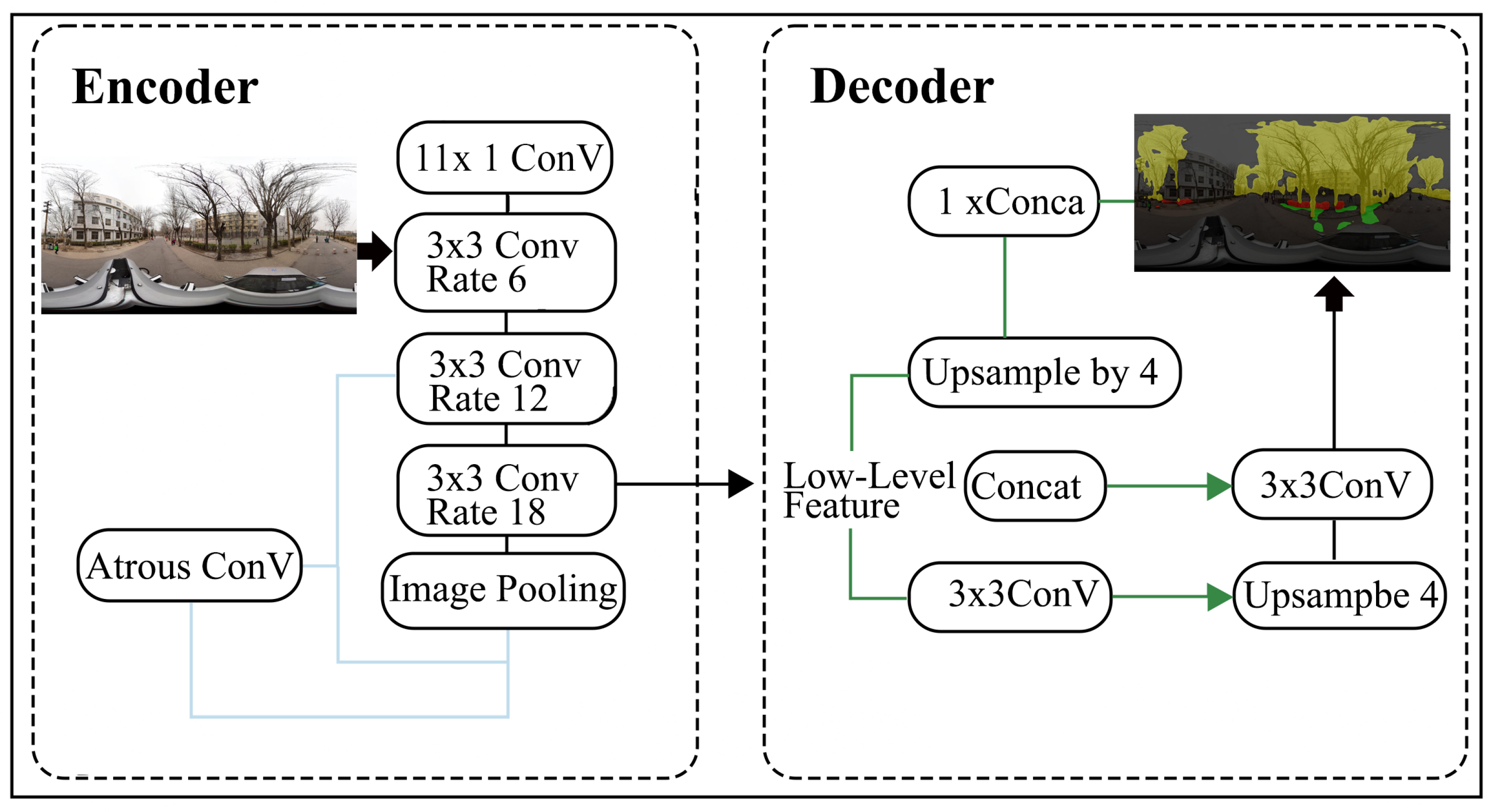
To construct greening structure variables at the street scale, we apply DeepLabv3+ [] for semantic segmentation of street-view images. The architecture uses atrous convolutions and atrous spatial pyramid pooling (ASPP) to capture multi-scale contextual information, while a decoder with learnable upsampling refines object boundaries to achieve high-precision, pixel-level predictions. Compared with mainstream segmentation baselines such as PSPNet and SegNet, as well as traditional classifiers (e.g., SVMs and random forests), DeepLabv3+ typically delivers higher segmentation accuracy and robustness in complex urban scenes, making it well suited to our need to identify fine-grained vegetation strata Figure 5. For data and training, we use the Street Greening Space Structure (SGSS) dataset developed by Zhang et al. [] as the pretraining corpus. Designed for street-scale greening measurement, SGSS integrates urban landscape scenes, Google Street View panoramas, and real-world photos, spanning urban, rural, campus, and residential contexts to enhance model transferability and generalization across street types. After 2000 training iterations, the model achieves validation metrics of mIoU = 0.630 , mPA = 0.7287 , Recall = 0.720 , and Precision = 0.807 . These results indicate that both inter-class separability and overall recognition accuracy meet the requirements for subsequent quantitative analysis.
Figure 5. DeepLabV3+ neural network structure.

3. Methodology

3.1. Street-Greening Structure Indicators

Street-greening structure indicators are computed from semantic-segmentation results on street-view imagery, using a DeepLabv3+ [] model trained on the SGSS dataset specifically optimized for urban greening measurement. Based on the segmentation outputs, we construct three fundamental view indices: the Tree View Index (G_TVI), the Bush View Index (G_BVI), and the Grass View Index (G_GVI). These indices measure, for each street-view image, the percentage of pixels visually occupied by trees, shrubs, and grass, respectively, as defined in Equation (1):
V I o b j , i = A r e a o b j , i A r e a t o t a l , i × 100 % , o b j { tree , bush , grass } .
Here, A r e a o b j , i denotes the number of pixels in the i-th image that are assigned by semantic segmentation to category o b j (where o b j = tree, bush, or grass), and A r e a t o t a l , i is the total number of pixels in that image. This yields the tree, shrub, and grass visual-coverage indices (G_TVI), (G_BVI), and (G_GVI), respectively.
Compared with the coverage rate of a single vegetation type, ratio-based structural indicators can reveal configuration relationships across vegetation strata. Accordingly, we compute the composite index of trees–shrubs–grass (G_TBG), the tree-to-shrub ratio (G_TBR), and the shrub-to-grass ratio (G_BGR). G_TBG captures the overall level of trees, shrubs, and grass, reflecting the comprehensive degree of street greening; G_TBR emphasizes the proportional balance between trees and shrubs, indicating coordination in the vertical stratum; and G_BGR reflects pairing at the near-ground stratum between shrubs and grass. As in related studies, ratio metrics can be distorted when denominators are very small []. To avoid this, we exclude low-denominator samples when computing G_TBR and G_BGR, ensuring stable indicator distributions. Considering the strong algebraic correlation between the tree–grass ratio (G_TGR) and the two ratios above, which could introduce multicollinearity in model estimation, we do not include G_TGR in the final indicator set. In practice, G_TBR and G_BGR sufficiently represent configuration in the vertical and near-ground strata, meeting the measurement needs for street-greening structure. Importantly, these ratio-based indicators are also managerially translatable: G_TBR (tree-to-shrub) aligns with maintenance mixes for upper and near-ground layers, such as appropriate tree spacing, crown raising, and continuous pruning; G_BGR (shrub-to-grass) maps to operations constraints, including shrub density, the share of permeable turf, and the width of sight corridors; G_TBG (total) provides an upper bound and marginal reference for overall greenery. Thus, the indicators measure not only “how much green” is present but also “how to configure maintainable structural combinations,” facilitating implementation as parameterized rules in planning, design, and maintenance, as defined in Equation (2).
G _ T B G = G _ T V I + G _ B V I + G _ G V I , G _ T B R = G _ T V I G _ B V I , G _ B G R = G _ B V I G _ G V I .
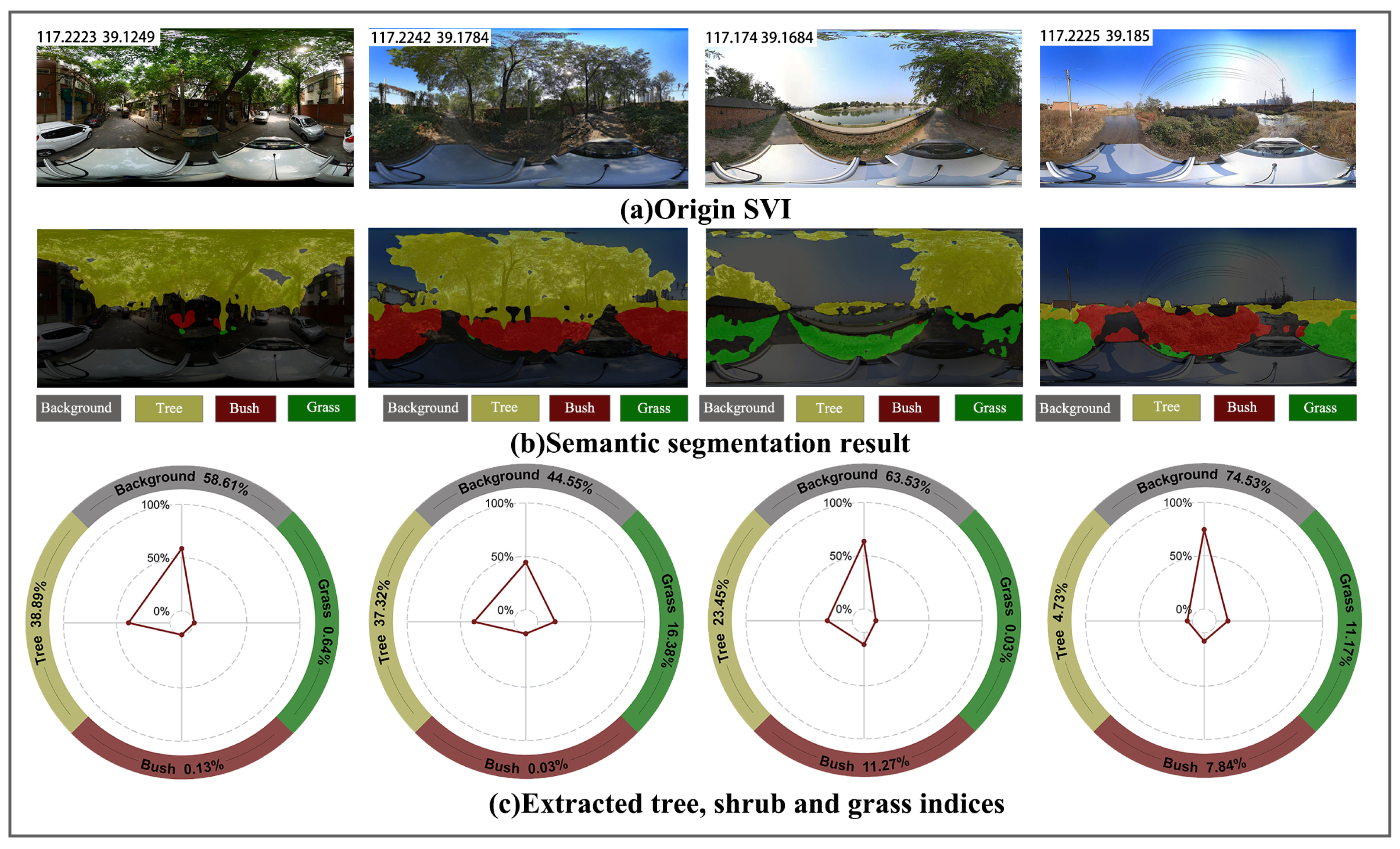
To validate the effectiveness of the semantic-segmentation results, we randomly selected four representative street-view images (SVIs) and plotted each image’s original photo, its segmentation output, and the distributions of the three vegetation indices (G_TVI, G_BVI, G_GVI). Manual comparison confirmed the reliability of the constructed greening structure indicators. We then diagnosed full-sample distributions and outliers for each indicator using standardized boxplots. For ratio-based indicators susceptible to very small denominators, we applied threshold-based exclusion and truncation to prevent disproportionate influence from a tiny amount of shrubs or grass (i.e., ratio blow-ups) that could adversely affect subsequent models. To further assess validity, we computed Pearson correlation coefficients between greening metrics and housing prices to explore potential linear associations and to inform subsequent nonlinear modeling. To visualize the spatial distribution of greening structure—and to reflect residents’ exposure within everyday activity ranges—we overlaid a regular 200 m × 200 m grid across the study area and mapped indicator values from each street-view sampling point to its corresponding grid cell. We then calculated cell-level averages for each indicator to reveal fine-scale spatial variation. The 200 m scale approximates a 2–3 min walking range, balancing detail and pattern readability in maps. Note that this gridding step is used solely for visualization in the results section and does not define the global spatial unit for model estimation. Aggregation was implemented in ArcGIS 10.8 and Python 3.8, and visualizations employed two-dimensional choropleth mapping and three-dimensional bar charts to illustrate the spatial distribution characteristics of the greening structure indicators.

3.2. Housing-Price Model

Following classical hedonic pricing theory, housing is treated as a heterogeneous good composed of measurable attributes, and its price is determined by three sets of variables: structural, locational, and neighborhood attributes []. Based on homebuyers’ preferences for specific housing characteristics, structural attributes describe the physical features of the dwelling, whereas locational attributes describe its position within the city. These are included as control variables to net out inherent housing differences and thereby enable more reliable identification of street-environment effects. Neighborhood attributes characterize the density and accessibility of key facilities and services. To distinguish conceptually from traditional neighborhood variables (amenity density and accessibility) and to highlight the structural-scale effects of street greenery, we treat street-view attributes as a separate category. Given our objective of systematically quantifying street-greening structure, the street-view attributes include three indicators—trees, shrubs, and grass—operationalized via the composite Tree–Shrub–Grass index (G_TBG), the Tree–Shrub ratio (G_TBR), and the Shrub–Grass ratio (G_BGR), which together clarify the contribution of greening configurations Equation (3).
PRICE = α + β 1 STRU + β 2 LOCA + β 3 NEIG + β 4 STRE + ε .
Here, α is the constant term; STRU, LOCA, NEIG, and STRE denote vectors of structural, locational, neighborhood, and street-greening structure attributes, respectively; β 1 β 4 are the corresponding coefficient vectors; and ε is the error term.
To assess the explanatory power of street-greening structures for housing prices, we first conducted preliminary tests by adding four categories of variables to separate OLS specifications to gauge their individual contributions. We then built a baseline model consisting of structural, locational, and neighborhood attributes, and subsequently introduced street-greening structure variables to test whether their inclusion improves the housing-price model. Note that urban spatial data commonly exhibit spatial dependence, which violates a core OLS assumption and may lead to biased coefficient estimates [,]. Accordingly, global OLS is used solely as a benchmark to examine the incremental contribution of street-greening structure to price determination. To mitigate potential multicollinearity arising from strong correlations among regressors, we performed variance inflation factor (VIF) diagnostics on the housing-price variable and all candidate covariates prior to model estimation to ensure the robustness of regression results. For instance, total green coverage (G_TBG) exhibits high collinearity with tree, shrub, and grass visibility; therefore, we separately assessed the incremental contributions of green visibility and hierarchical structure to the housing-price model []. To detect potential spatial effects, OLS residuals were subjected to Moran’s I and Lagrange multiplier tests to verify spatial autocorrelation and spatial dependence.

3.3. Geographical-XGBoost

Although the OLS model provides a baseline reference for the marginal effects of street-greening structures, it struggles to accommodate nonlinear relationships and spatial heterogeneity among variables. Geographically weighted regression (GWR) and its semiparametric extension (SGWR) are effective for revealing spatial non-stationarity; however, because they rely on linear specifications, they are limited in capturing nonlinear effects and higher-order interactions, which constrains their ability to model complex spatial relationships []. To overcome these limitations and to capture both overall trends and local spatial heterogeneity in the determinants of property prices, a more comprehensive assessment of street-greening impacts is required. This paper employs the Geographical-XGBoost (G-XGBoost) model proposed by Grekousis [], which combines XGBoost’s nonlinear learning capacity with geographically weighted local regression. By introducing spatial weights, fitting local submodels, and assembling a global–local prediction framework, G-XGBoost characterizes spatially heterogeneous response patterns and relationships. Within G-XGBoost, standard XGBoost serves as the global learner to capture the overall trend in housing prices. Its predicted values are expressed in Equation (4):
y ^ i gl = k = 1 K f k ( x i ) , f k F .
Among these, y ^ i gl denotes the global prediction for sample i; f k is the k-th CART regression tree; K is the total number of trees; and F is the space of admissible regression trees. At the street scale, residents’ perceptions and accessibility propagate along road networks rather than straight lines. For example, two locations separated by a river or a railway may be close in Euclidean terms yet remain inaccessible on foot. To align the modeling neighborhood with this practical mechanism, we measure geographic proximity using the shortest distance along the road network, as in Equation (5):
d i j net = dist sp i , j G ,
Here, G denotes the road graph derived from the OSM road network, and dist sp represents the shortest-path length on this graph. Building on this, we transform network distance into a decaying weight via an adaptive kernel K ( · ) with location-specific bandwidth b i Equation (6):
w i j = K d i j net b i , K bisq ( u ) = ( 1 u 2 ) 2 I ( u < 1 ) or K gauss ( u ) = exp 1 2 u 2 ,
The former assigns zero weight outside u 1 (compact support with a clearly defined neighborhood), whereas the latter decays smoothly (thus distant samples exert minimal influence). To obtain an unbiased evaluation of local fit and to avoid self-reinforcement, and given the coexistence of dense road networks in the old city and relatively sparse corridors on the periphery, the neighborhood size should not be fixed. We set w i i = 0 so that the focal observation serves as an out-of-bag (OOB) sample; optionally, imposing j i w i j = 1 enables comparability across locations. Bandwidth employs a k-nearest-neighbor adaptive rule (e.g., k = 80 ): let d i ( k ) net denote the network distance from point i to its k-th nearest neighbor, and define bandwidth selection as in Equation (7):
b i = d i ( k ) net , k = arg min k K CV ( k ) ,
Global hyperparameters are tuned via nested cross-validation combined with grid search and then applied to the local models to mitigate overfitting. Here, K denotes the candidate neighbor set (e.g., { 50 , 75 , , 250 } ). In nested cross-validation (Nested CV), the inner CV searches for optimal hyperparameter combinations, while the outer CV evaluates their generalization performance. The selection of k proceeds by minimizing the cross-validated mean squared error in Equation (8):
CV ( k ) = 1 n i = 1 n y i y ^ i loc ( k ) 2 ,
Here, y ^ i loc ( k ) denotes the local prediction obtained by training with b i = d i ( k ) net . Unlike GWR, where residuals are weighted in a weighted-least-squares objective, the weights here enter the gradient and Hessian, thereby affecting node-split gains and enabling nonparametric learning of nonlinearities and interactions under spatial heterogeneity. Based on this weighting scheme, we embed w i j directly into XGBoost’s first- and second-order derivatives to obtain the geographically weighted local objective in Equation (9):
L i loc = j = 1 n i g j w i j f t ( x j ) + 1 2 h j w i j f t 2 ( x j ) + Ω f t ,
Here, g j and h j denote the first- and second-order gradients, respectively; f t ( x j ) is the prediction of the t-th regression tree for sample j; and Ω ( f t ) is the regularization term. Unlike standard XGBoost, G-XGBoost embeds spatial weights directly into the gradient (and Hessian) computations, enabling the model to emphasize nearby samples that contribute more to the prediction error during training. Concretely, the local model introduces spatial weights when computing feature importance by applying a weighted adjustment to XGBoost’s gain metric, thereby yielding spatially weighted local feature importance. This quantifies how the contribution of each feature varies across locations. In contrast to the permutation-based importance used in Geographical Random Forests (GRFs), this approach directly reflects how spatial heterogeneity modulates feature contributions within the boosting process. Finally, G-XGBoost dynamically fuses global and local predictions using a weighting coefficient α i [ 0 , 1 ] , which preserves local detail while controlling variance instability in sparse neighborhoods. The ensemble prediction is a convex combination of the two components, as shown in Equation (10):
y ^ i ens = α i y ^ i loc + ( 1 α i ) y ^ i gl .
Here, α i [ 0 , 1 ] can be fixed or adaptively adjusted based on the residual magnitude between the local and global predictions. When the local model underperforms, increasing the global weight improves overall accuracy; conversely, assigning a larger weight to the local model captures fine-grained spatial variation. This design enforces neighborhood definitions consistent with actual reachability, supports robust bandwidth selection under uneven network density, and automatically increases the global weight in information-sparse regions. In this way, the approach balances global stability and local heterogeneity without relying on linear assumptions.
This study integrates the SHAP interpretability framework with the XGBoost model to analyze the contribution and impact of individual features on predictions, thereby enhancing interpretability. SHAP increases the transparency of “black-box” models by quantifying each feature’s marginal contribution to the model output, offering global and local perspectives on feature importance. Each feature is treated as a “contributor” to the prediction; its SHAP value reflects the positive or negative effect of that feature for a given instance, providing an intuitive and quantitative interpretive mechanism []. For data partitioning, the dataset was split into a 70% training set and a 30% test set to ensure robustness and generalization.During training, nested cross-validation combined with grid search was used to tune G-XGBoost hyperparameters (n_estimators = 600, learning_rate = 0.01, max_depth = 7, min_child_weight = 5, gamma = 0, subsample = 0.6) to mitigate overfitting risk, improving adaptability and predictive performance in complex feature spaces. Spatial visualization of SHAP values from the local G-XGBoost models substitutes for traditional GWR coefficient maps, directly quantifying each variable’s positive or negative contribution to predictions. This approach avoids interpretability pitfalls of linear models under standardization or multicollinearity and addresses GWR’s limitations in modeling nonlinear spatial processes stemming from its linear assumptions.
Regarding model interpretation, this study analyzes the mechanisms of street-greening structure at three levels: global, local, and interactive. First, the global G-XGBoost model is used to produce SHAP beeswarm plots, providing a comprehensive comparison of feature importance and visually situating the contribution of greening structure relative to structural, locational, and neighborhood attributes in predicting housing prices. Second, Partial Dependence Plots (PDPs) are generated to reveal the nonlinear effects of individual features on predicted prices and to identify potential thresholds. Finally, SHAP interaction plots are employed to examine synergistic or substitutive relationships among variables, thereby uncovering the complex interplay between greenery structure and other determinants of housing prices.

4. Results

4.1. Validation and Spatial Analysis of Street-Greening Indicators

As shown in Figure 6, cross-validation supports the reliability of the semantic segmentation. The outputs successfully distinguish trees, shrubs, and grass across different street-view images. For example, the first two images depict street segments with dense tree canopies, whereas the third and fourth images show more open scenes with more prominent shrub and grass coverage. These visual impressions are accurately reflected in both the semantic-segmentation results (Figure 6b) and the extracted greening indices (Figure 6c). Radar charts provide further quantitative validation: in tree-dominated environments (the first two samples), G_TVI is 38.89 % and 37.32 % ; the corresponding G_BVI values are 0.13 % and 0.03 % , and G_GVI values are 0.64 % and 16.38 % . By contrast, the third and fourth samples show reduced tree coverage— 23.45 % and 4.73 % —with marked increases in shrubs and grass G_BVI = 11.27% and 7.84%; G_GVI = 0.03% and 11.78%. This shift from tree-dominated to more balanced tree–shrub–grass distributions aligns with the visual characteristics of more open landscapes, demonstrating that the DeepLabv3+ model not only identifies primary greenery elements but also captures structural differences between street scenes at a quantitative level.
Figure 6. Samples of (a) origin SVI, (b) semantic segmentation result, (c) extracted tree, shrub and grass indices. The radar chart shows the scores from 0% to 100% from the inside out.
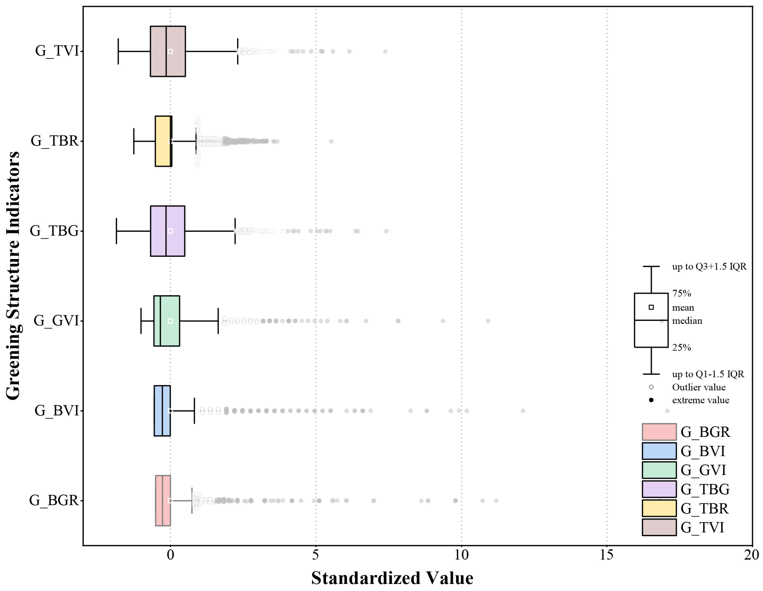
To further reveal the overall distributional characteristics and differences among greening structure indicators, standardized boxplots, shown in Figure 7, present the statistics for six indicators in the study area. The pattern conforms to a typical “tree-dominated, shrub–grass sparse, long-tailed ratios” distribution []. Among the basic view indices, G_TVI has the highest median and a relatively wide interquartile range (IQR), indicating widespread tree presence but substantial variability in exposure. By contrast, G_BVI and G_GVI have medians close to zero with narrow IQRs, and only a few high-value outliers on select segments, reflecting limited shrub and grass configurations with spatially concentrated occurrence. Among structural indicators, the distribution of G_TBG closely mirrors that of G_TVI, implying that overall visible greenery is primarily driven by the tree layer. Notably, the ratio indices G_TBR and G_BGR display pronounced long-tailed distributions with numerous extremes, revealing marked imbalances between tree–shrub or shrub–grass strata on certain segments. Overall, the boxplots highlight core features of Tianjin’s street greening: trees constitute the dominant element, shrub and grass layers are generally underprovided, and some segments exhibit significant stratification imbalances.
Figure 7. Standardized boxplots of six greening structure indicators.
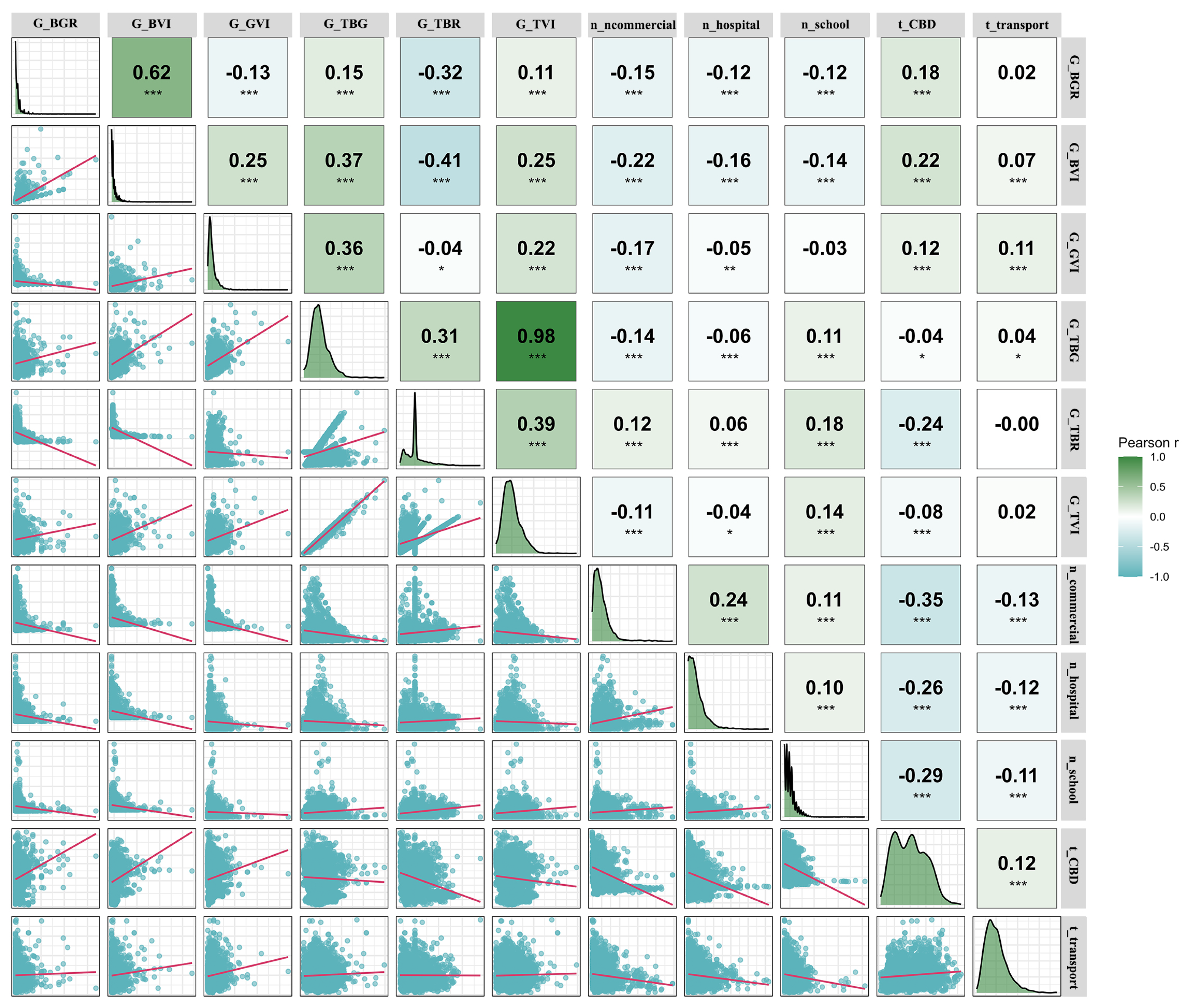
Coefficients are shown in Figure 8. Overall, correlations within the greening indicators are generally strong, whereas correlations with housing-price-related variables are weak, with most | r | values below 0.4. Within the greening set, a clear pattern emerges: the tree layer dominates overall visible greenery. In particular, G_TVI and G_TBG are nearly perfectly correlated ( r = 0.98 ), indicating that overall greening is primarily determined by trees. By contrast, G_TBR is negatively correlated with shrub and grass indicators, reflecting a trade-off between ratio-based and ground cover measures.Relative to housing-price variables, greenery indicators exhibit weaker correlations. Most indicators show slight negative correlations with non commercial POIs and medical facilities; correlations with school counts are close to zero. Distance to the CBD shows weak positive correlations with tree and composite greening indicators ( r 0.2 ), but weak negative correlations with ratio-based indicators. Correlations between traffic accessibility and all greening indicators are near zero. Taken together, the Pearson results indicate strong internal correlation within greening structure, especially the decisive role of trees in overall visible greenery, yet only limited linear association with housing-price-related variables [,].
Figure 8. Pearson correlation matrix of six greening indicators and housing-related variables. Values indicate correlation coefficients, with significance levels marked (* p < 0.1; ** p < 0.05; *** p < 0.01). Diagonal plots show variable distributions, and lower panels show pairwise scatter plots with fitted regression lines.
Figure 9 displays the spatial distribution of greening structure indicators across six street categories within Tianjin’s six urban districts at a 200 m × 200 m grid resolution. Overall, notable spatial heterogeneity is evident, with clear differentiation in indicator values between core and peripheral zones and discernible clusters of high and low values. For tree-related indicators (G_TVI, G_TBG), higher values are continuously observed in central districts such as Heping, Hexi, and Nankai, forming banded patterns that are consistent with documented mature street-tree systems in core areas [,]. In contrast, Hebei, Hedong, and Hongqiao tend to show lower levels overall, with scattered high-value units on only a few segments []. For shrub and grass indices (G_BVI, G_GVI), a low-value background is prevalent, with only dispersed clusters of higher values in open spaces or along peripheral waterfronts. The limited continuity of the shrub–grass layer aligns with the concentrated distributions and long-tailed outliers seen in the boxplots, and it is consistent with prior findings on relatively monotonous street-greening structures []. Among ratio-based indicators, higher G_TBR values are scattered across central and northern urban areas, suggesting local imbalances in tree-to-shrub ratios, whereas higher G_BGR values appear more often in peripheral areas, suggesting shrub dominance relative to grass. Taken together, the six urban districts exhibit a spatial pattern characterized by tree dominance in central zones, sparser shrub–grass coverage in peripheral zones, and dispersed ratio-based indicators, indicating pronounced spatial heterogeneity in greenery stratification.
Figure 9. Three-dimensional and planar spatial distribution of six greening structure indicators across Tianjin. (a) Greening Visibility Index, (b) Greening Stratification Structure Index.

4.2. Spatial Housing-Price Modeling Results

As shown in Figure 3, housing prices in Tianjin’s six urban districts display pronounced spatial clustering. In general, prices form a gradient that decreases from the central business district (CBD) toward the periphery, with higher values concentrated in core urban areas and lower values more prevalent in marginal zones. The global Moran’s I statistic ( Moran s I = 0.76 , p < 0.001 ) indicates strong positive spatial autocorrelation in housing prices, that is, both high-value and low-value properties tend to cluster. The LISA clustering map (Figure 3d) further reflects this pattern: higher-priced blocks are concentrated in districts near the CBD, such as Heping, Nankai, and Hexi, whereas lower-priced areas cluster in peripheral districts including Hebei, Hongqiao, and Hedong. Overall, this spatial arrangement is consistent with Tianjin’s traditional center–periphery urban structure.
Table 4 reports OLS fitting performance and diagnostics for the four attribute groups. Overall, locational attributes show the highest explanatory power (adjusted R 2 = 0.497 ), followed by neighborhood attributes (0.356), green-structure attributes (0.254), and structural attributes (0.244). Residuals from all models exhibit significant spatial autocorrelation, with Moran’s I z-scores exceeding 85 ( p < 0.01 ) , indicating that linear OLS specifications inadequately capture spatial dependence. Robust Lagrange multiplier tests further indicate significant spatial effects in both lag and error components (e.g., structural attributes: LM–lag = 588.935 , LM–error = 15.325 ; neighborhood attributes: LM–lag = 361.010 , LM–error = 373.068 ), suggesting that spatial processes are non-negligible across attribute-specific models. Although all four attribute groups are statistically associated with housing prices, the OLS spatial diagnostics motivate explicit spatial modeling. Accordingly, subsequent analyses incorporate structural, neighborhood, and locational attributes into a baseline model that serves as the reference framework for comparisons with green-structure specifications and G-XGBoost.
Table 4. Regression performance and diagnostic results across different OLS models.
Within this spatial context, structural, locational, and neighborhood attributes were first incorporated into an initial OLS specification to construct the baseline model (Model 0). This model explains approximately 55.1 % of the variation in housing prices. Subsequently, the total greening indicator and the hierarchical structure indicator were introduced into the regression framework, yielding expanded models (Model 1 and Model 2) to test the incremental marginal effect of overall greening on housing-price modeling. The regression results (Table 5) show that Model 2 increases explanatory power to 57.2 % , an improvement of 0.021 over the baseline, indicating that incorporating green-structure variables enhances predictive performance. This is consistent with evidence on tree cover and housing prices reported by Lin []. Moreover, Moran’s I and robust Lagrange multiplier diagnostics on OLS residuals indicate significant spatial autocorrelation. For both the baseline and the green-structure-augmented models, Moran’s I tests are highly significant ( p < 0.01 ) , suggesting that residuals retain strong spatial clustering. Robust LM tests also indicate significant spatial lag and spatial error components (e.g., Model 0: LM–lag = 251.649 , LM–error = 106.400 ; Model 1: LM–lag = 341.987 , LM–error = 122.081 ), implying that spatial processes are non-negligible. Taken together, these diagnostics suggest that the relationship between housing prices and street-greening structure is not spatially homogeneous but exhibits notable spatial non-stationarity, motivating the use of spatial regression and nonlinear models for further analysis [].
Table 5. Regression results and diagnosis. Regression performance and diagnosis for all OLS, and G-XGBoost models.
To address the limitations of OLS in handling spatial dependence and nonlinear effects, this study adopts the Geographical-XGBoost (G-XGBoost) framework. During training, the optimal bandwidth was selected via cross-validation as k = 156 , and an adaptive kernel was used to weight estimates across locations. Table 6 reports predictive performance for the global and local G-XGBoost models. For the global model, R 2 = 0.634 and adjusted R 2 = 0.625 , improving upon the OLS baseline ( R 2 = 0.551 ) ; meanwhile, MAE and RMSE decrease to 0.254 and 0.325 , and MAPE declines to 2.46 % . These results indicate that incorporating nonlinear learning better captures the complex associations between greening structure and housing prices. In comparison, the local G-XGBoost model shows further gains in fit. With spatial weighting via the adaptive kernel, the local model attains overall R 2 = 0.780 and adjusted R 2 = 0.774 , with additional reductions in prediction error (MAE = 0.186 , RMSE = 0.252 , MAPE = 1.79 % ). This pattern is consistent with spatial variation in the relationships within the six urban districts, which the local specification captures more precisely. Overall, interpretability and out-of-sample accuracy increase progressively from OLS to global G-XGBoost to local G-XGBoost, suggesting that combining nonlinear learning with spatial localization is effective for representing spatial differences reflected in the model.
Table 6. Comparison of prediction performance between global and local G-XGBoost models.
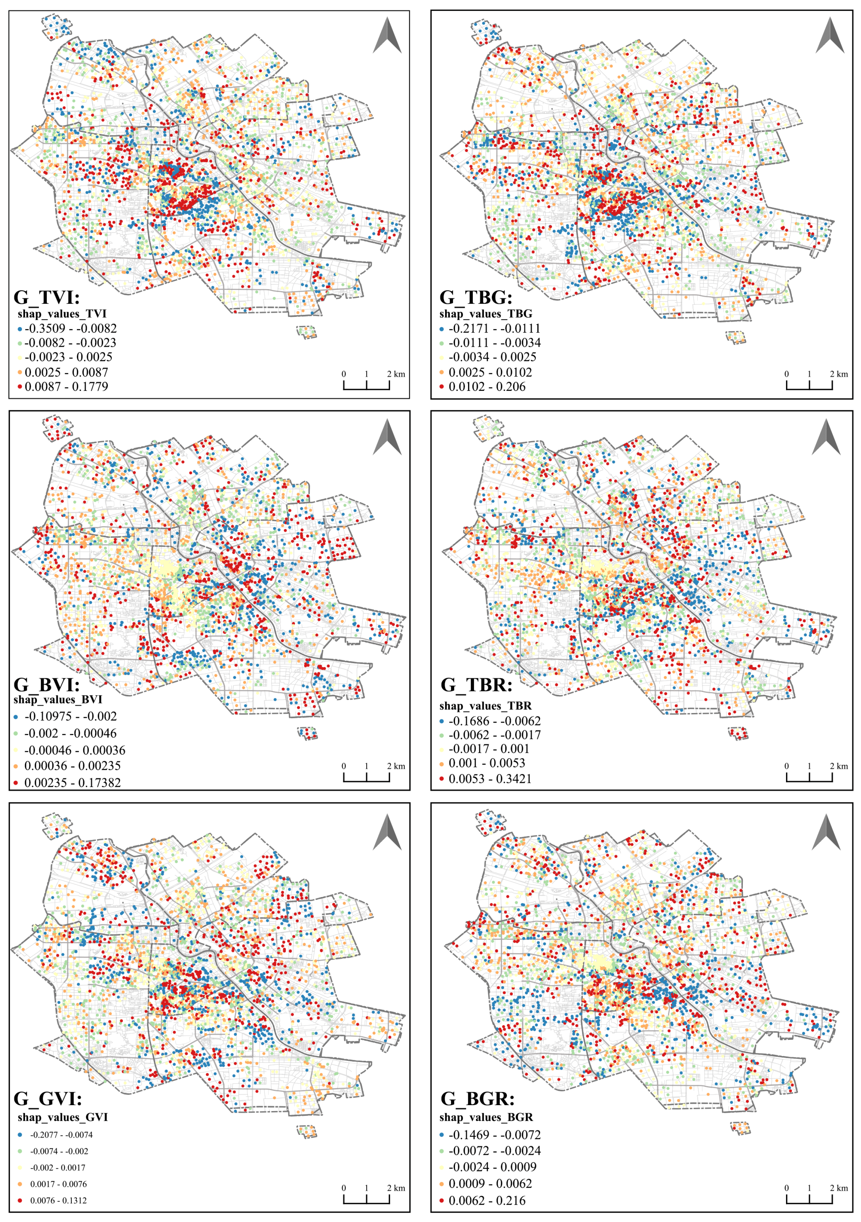
To visualize spatial heterogeneity in the relationship between greenery structure and housing prices—and to obtain a display functionally comparable to GWR’s local coefficient maps within the G-XGBoost framework—we use SHAP values from the local G-XGBoost model to map the spatial patterns of six greenery structure indicators, as shown in Figure 10. Analogous to how traditional GWR employs local regression coefficients to summarize direction and magnitude, SHAP values provide point-level indications of each indicator’s positive or negative contribution to predicted prices and its relative strength: warm colors denote positive contributions, cool colors denote negative contributions, and color intensity represents magnitude. This visualization highlights differences in direction and intensity across areas within the six urban districts and thus makes spatial heterogeneity more apparent.The resulting “contribution–space” patterns display notable non-stationarity with zoned clustering. Tree-related indicators (G_TVI, G_TBG) show highly consistent spatial distributions. This pattern aligns with the high exposure and banded canopy distributions observed in central areas, where tree visibility and the composite greenery it dominates are more often associated with positive contributions; in peripheral areas, marginal contributions are less stable and contribution signs vary. Shrub and grass indices (G_BVI, G_GVI) generally present weak backgrounds, with localized positive clusters near urban fringes or open spaces, while core areas more often exhibit weak negative or negligible contributions. The two ratio indicators (G_TBR, G_BGR) differ markedly from the base indices: contributions are both positive and negative and are highly dispersed, appearing as patches or points rather than continuous bands. G_TBR shows positive patches on some central–northern segments and negative contributions elsewhere; G_BGR’s positive patches are more frequently observed in peripheral areas, whereas core zones tend to exhibit weak or negative contributions. Overall, across the six indicators, the contribution–space relationship exhibits pronounced spatial non-stationarity: tree-dominated indicators (G_TVI, G_TBG) concentrate in stable positive clusters in core areas; shrub and grass indicators (G_BVI, G_GVI) show localized positive contributions around peripheral or open environments with weaker or negative values in cores; and ratio indicators (G_TBR, G_BGR) are characterized by dispersed, bidirectional patches, reflecting localized thresholds and contextual dependence in allocation structures.
Figure 10. Spatial distribution of SHAP values from the local G-XGBoost model for six greening indicators. Warm (cool) colors denote positive (negative) contributions to predicted housing prices; color intensity indicates magnitude.

4.3. Contributions and Interaction Effects of Street-Greening Structure on Housing Prices

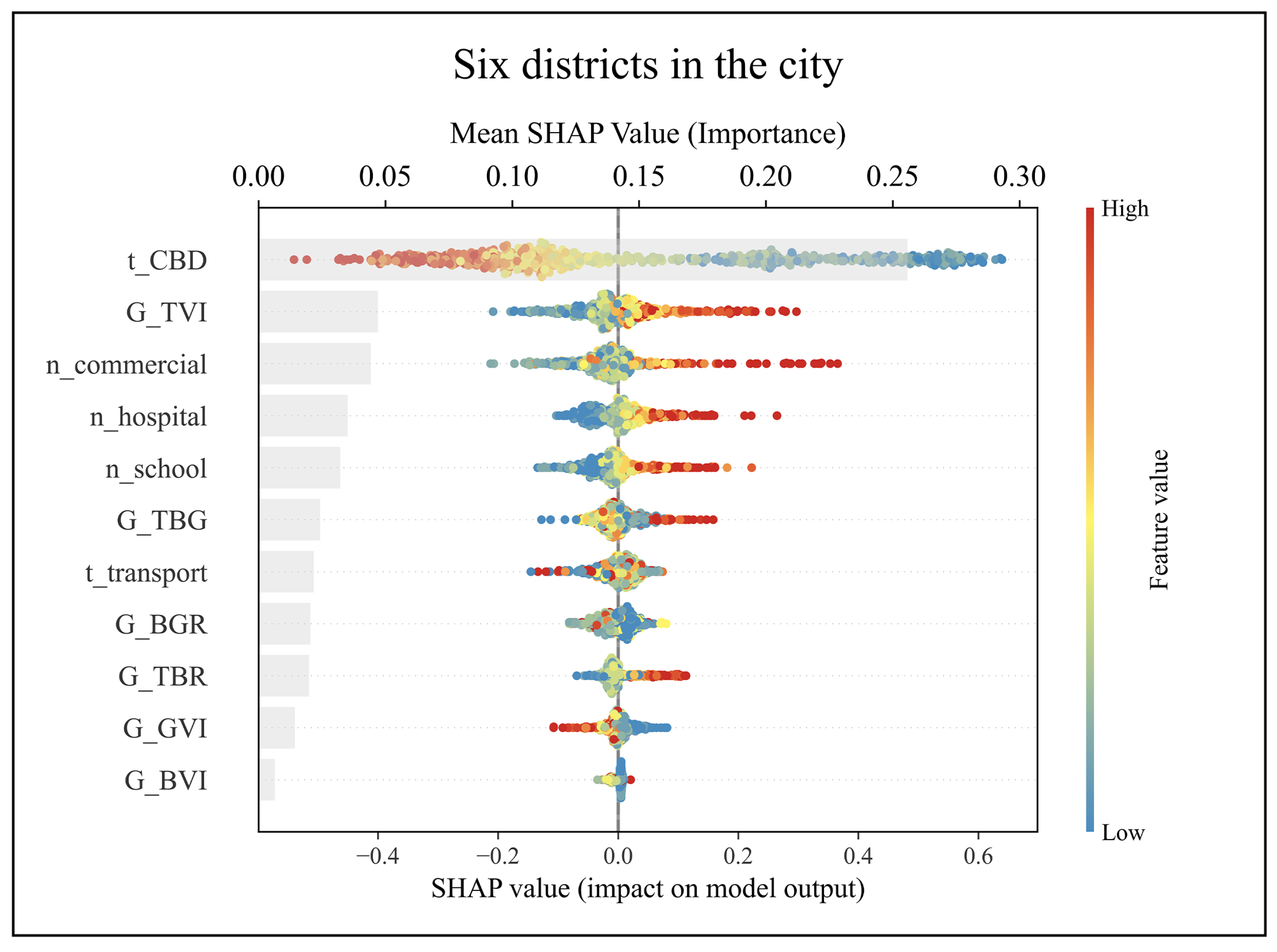
To quantify the share, directional influence, and importance of street-greening structures within the housing-price model, we compute SHAP values using the global G-XGBoost and plot a SHAP summary (beeswarm) diagram, as shown in Figure 11. The diagram simultaneously visualizes variable importance, directionality, and impact distribution: background gray bars represent mean absolute SHAP values (global contribution); the horizontal axis shows SHAP values, indicating each variable’s positive or negative effect and its magnitude on predicted prices; the vertical axis ranks variables by importance from top to bottom; scattered colors encode feature values from low (light) to high (dark). Overall, among locational factors, distance to the CBD (t_CBD) ranks first and shows a clear monotonic pattern: shorter distances are associated with more positive effects on predicted prices, whereas greater distances (high values, red) align with negative effects. Among greening variables, the Tree View Index (G_TVI) exhibits the highest mean contribution, with most high-value points on the positive side. The composite greening measure (G_TBG) shows a similar but weaker distribution, suggesting that highly visible and structurally stable tree canopies are more readily reflected in the model as price gains. Although correlated with G_TVI, key aspects of overall greenness are largely represented by G_TVI. Together with neighborhood facilities (commercial establishments, schools, hospitals), these variables form the second tier of contributors. Shrub and grass indicators (G_BVI, G_GVI) display weaker average contributions at the global scale; some high-value points trend slightly negative, which is consistent with limited price relevance in dense built environments. Ratio metrics (G_TBR, G_BGR) have shorter gray bars, indicating lower global mean contributions; their point clouds disperse on both sides of zero, with high values (red) appearing on both positive and negative sides, without the unidirectional gradient seen for G_TVI. This “low mean plus mixed sign” pattern suggests heterogeneous marginal contributions across samples that may depend on thresholds or context, which can be offset at the global scale.In sum, the beeswarm plot highlights tree-related indicators (G_TVI, followed by G_TBG) as the most informative greening signals for price prediction across the six districts. By contrast, shrub and grass exposure and ratio configurations contribute more weakly overall, while exhibiting mixed directions and threshold or context sensitivity. These observations guide the next section’s analysis: prioritize nonlinear response curves for G_TVI and G_TBG, and investigate thresholds and scenario dependence through pairwise interaction analysis for G_TBR and G_BGR.
Figure 11. SHAP beeswarm of the global G-XGBoost model. Predictors are ordered by mean absolute SHAP (gray bars); points show observation-level SHAP (x-axis: impact on predicted price; color: feature value; SHAP value log price, ln RMB/m2).
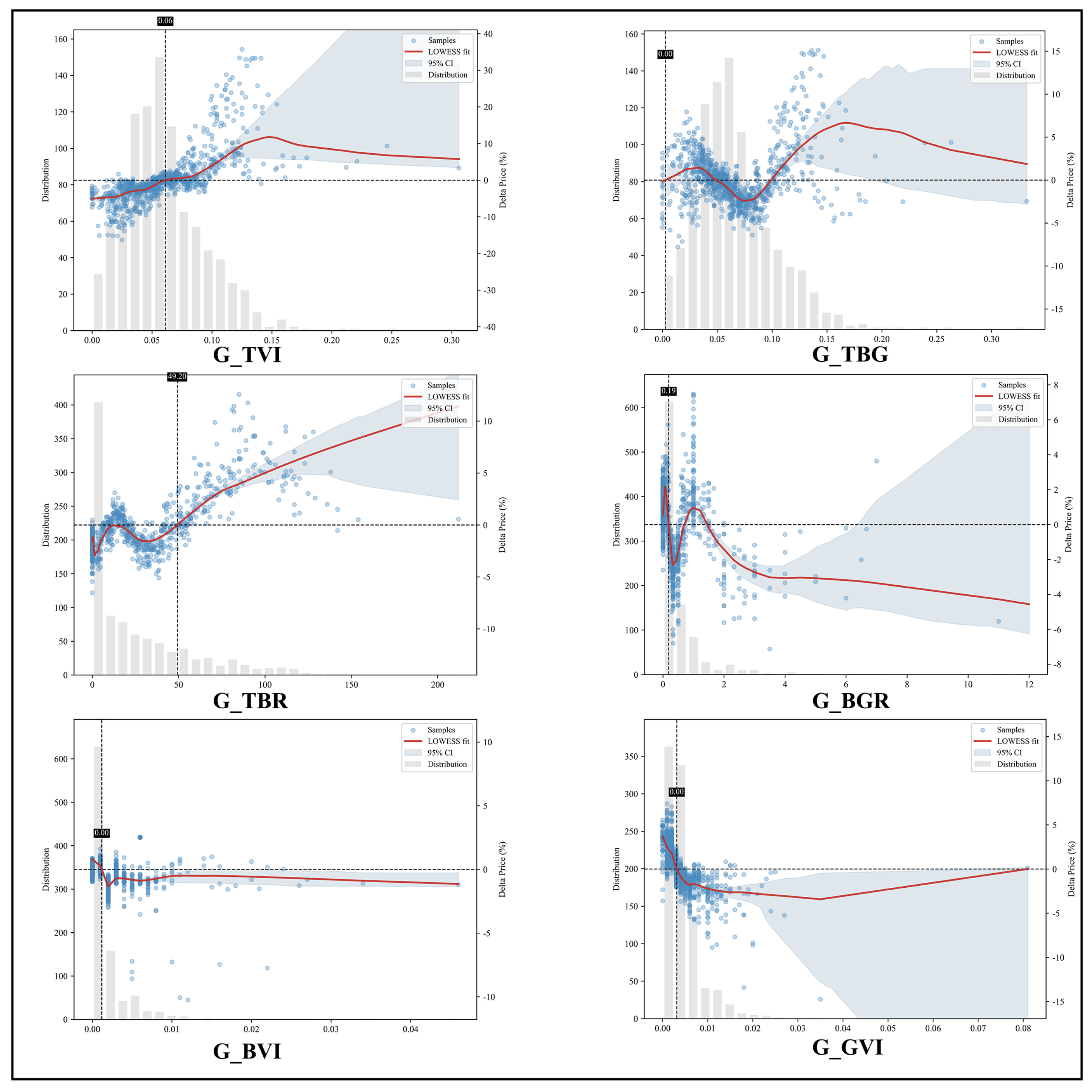
To assess the marginal impacts of six greening indicators on housing prices and examine nonlinear effects of street-greening structure, we use the global G-XGBoost model to plot nonlinear marginal response curves, as shown in Figure 12. The horizontal axis reports original indicator values; the right y-axis shows logarithmic contributions to housing prices converted to percentage changes; the gray histogram (left y-axis) depicts feature-value frequencies. For the tree-related indicator G_TVI, increases from about 0.06 to 0.12–0.16 are associated with price uplifts of roughly 8%–10%. Beyond 0.18, gains stabilize and taper, maintaining an uplift of approximately 6%–8%. G_TBG shows an effective gain band between 0.12 and 0.20, with an uplift of about 6%–8%; above 0.20, additional gains slow to roughly 2%–4%. These patterns indicate that highly visible, continuous tree layers are most readily reflected as price premia, with diminishing marginal gains at high exposure. Structural ratio indicators. The tree–shrub ratio (G_TBR) exhibits negative associations with price at low ratios; at around 30 it switches toward positive values and then increases, with an optimal range at 70–150 that corresponds to uplifts of 10%–12%. Above 150, the uplift plateaus and uncertainty increases. The shrub–grass ratio (G_BGR) shows a brief positive interval between 0.3 and 0.8; it turns negative above 1.0 and becomes more negative as the ratio rises, corresponding to reductions of about 3%–4% around 8–12. Overall, configurations in which trees dominate without excessively crowding shrubs appear most favorable, whereas strong shrub dominance over grass aligns with weaker price performance.For individual shrub/grass indicators, the net global effects are modest: G_BVI (shrub visibility) and G_GVI (grass visibility) show weak or insignificant global-level impacts. This suggests that isolated increases in shrubs or grass seldom yield consistent price gains; their influence is expressed primarily through proportional relationships and at extreme ranges.The marginal curves that indicate “moderate G_TBR performing best and excessive G_BGR being penalized” align with price signals and also suggest potential ecological implications: moderate tree–shrub ratios are more likely to form multi-layered canopies and traversable ground layers, which can support functional biodiversity and microclimate buffering to some extent; when G_BGR exceeds 1 (i.e., shrubs dominate grass), greater enclosure at ground level may increase wind resistance and compress corridors that serve both ecological and pedestrian functions, thereby weakening ecological connectivity and street accessibility, a tendency that corresponds economically to a discount.
Figure 12. SHAP dependence for six street-greening indicators (nonlinear marginal effects; log-price model; right axis = price change %, points = SHAP, red = LOWESS, shading = 95% CI).
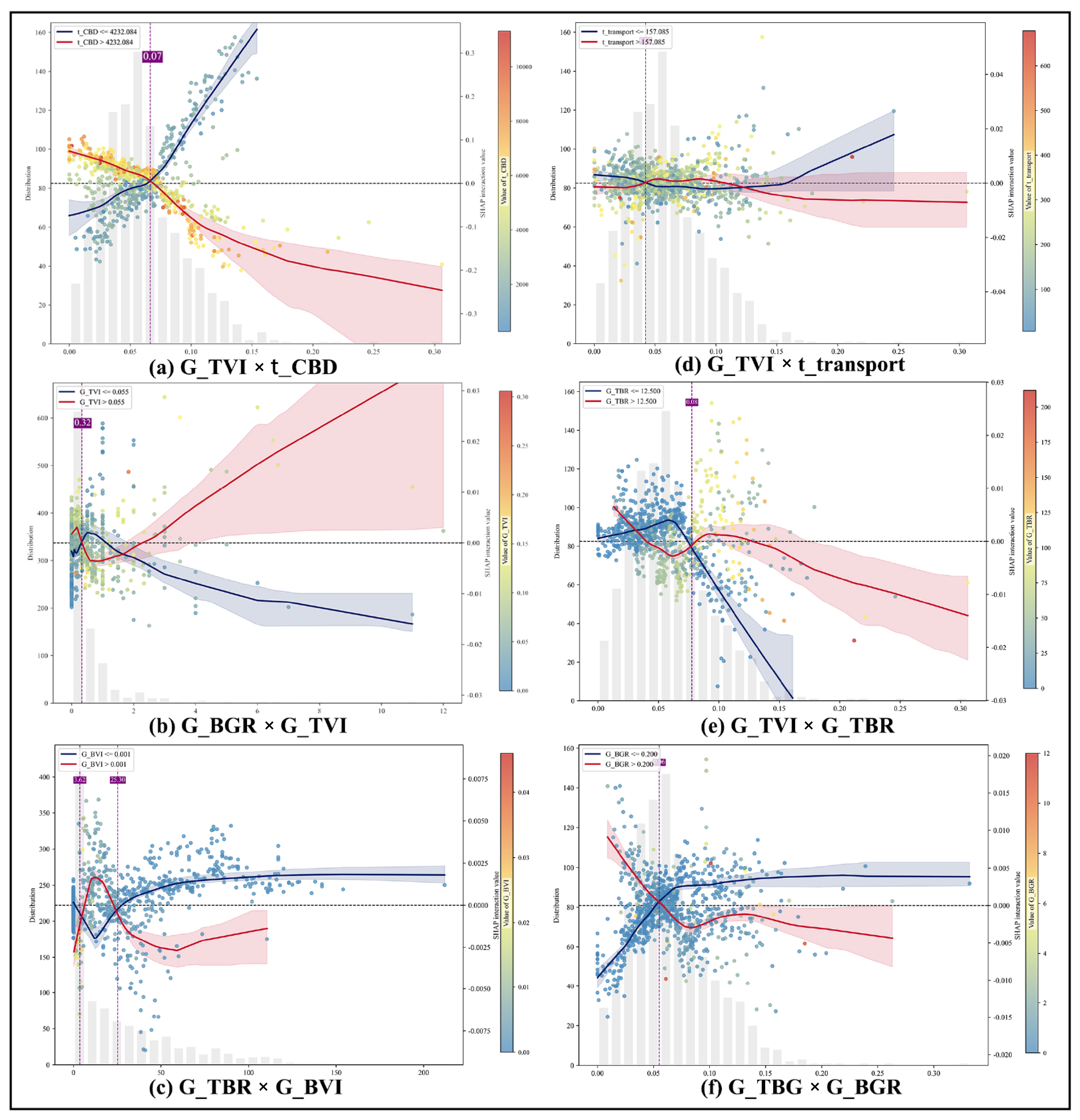
After confirming nonlinear marginal responses and critical thresholds, it is further necessary to assess their conditional stability and the direction of modulation by exogenous contexts from an interaction perspective. Accordingly, SHAP interaction values were computed using the global G-XGBoost model and plotted in a six-panel interaction dependency diagram, which reveals the “threshold–context” linkage mechanism and supports the extrapolation of prior conclusions, as shown in Figure 13. The x-axis shows original values of the primary variables, the right y-axis shows SHAP interaction values, and the left y-axis indicates sample frequency; scatter points are colored by the values of the interacting variable. Blue and red lines indicate locally smoothed trends for the low- and high-score groups, respectively (shaded areas denote uncertainty ranges). The purple dashed line marks the empirical threshold from the previous section. This configuration maintains focus on the research question, reduces informational redundancy and instability from many-to-many combinations, and preserves non-duplicative mechanisms with planning readability. We calculated interaction strengths for all pairwise combinations of “Green Structure × Location/Accessibility/Near-Ground Layer/Structural Ratio.” The results suggest a progressive pattern: Location and Accessibility first delimit the upper bound of potential gains, which are then modulated by the near-ground layer structure, and finally the internal structural ratios determine whether gains are stably activated. In near-CBD or transit-proximate contexts, exceeding the G_TVI threshold aligns with greater and more persistent price appreciation. For example, increasing G_TVI from approximately 0.06 to 0.12–0.16 corresponds to gains of about 10% near the CBD and about 6% farther from the CBD, as shown in Figure 13a,d. Second, the underlying stratigraphic structure relates to whether penalties are offset. When shrubs predominate over grass (i.e., BGR exceeds approximately 1) and G_TVI is low, property values show a slight decline in the high-BGR segment. Increasing G_TVI to around 0.10 largely neutralizes this negative tendency, as shown in Figure 13b. Finally, the internal structure exhibits a “premise–activation/erosion” relationship: TBR provides the premise, G_TVI functions as the activation term, and G_BGR/G_BVI constitute erosion terms. Elevated shrub visibility (G_BVI) compresses the optimal tree–shrub zone: at low BVI, TBR is associated with strong positive gains of roughly 10%; at higher G_BVI, gains within the same range are minimal and plateau earlier, as shown in Figure 13c. A similar pattern holds for composite greenery (G_TBG): only when G_BGR is low (around 0.20 or below) does the medium-to-high range of TBG stably correspond to price gains; when G_BGR is elevated, gains tend to flatten or turn negative, as shown in Figure 13e,f. In summary, on street segments with higher centrality or accessibility, enhancing tree visibility (G_TVI) corresponds to greater price returns. When G_BGR or G_BVI is elevated, shrub enclosure relates to weaker returns. Returns are most stable, with milder diminishing marginal effects, when the tree-to-shrub ratio (G_TBR) is moderate and configurations that avoid shrubs exceeding grass are employed.
Figure 13. SHAP interaction dependence plots for street-greening structure. Right Y-axis: Equivalent price change (%).

5. Discussion

5.1. Effects of Street-Greening Structure on Housing Prices

This study builds on prior research that measured street greening only by “green volume” or a single GVI metric. We propose decomposing greening structure into two observable dimensions: (i) visibility (G_TVI, G_BVI, G_GVI) and (ii) hierarchical proportion (G_TBR, G_BGR, G_TBG). Using G-XGBoost together with global and local SHAP, we jointly capture nonlinearity and spatial heterogeneity, thereby advancing the structure–price relationship beyond average effects to explain which structures act, where they matter, and how they influence prices, as shown in Figure 11, Figure 12 and Figure 13. First, tree visibility (G_TVI) remains robust across models and subsamples, consistent with multi-city evidence centered on canopy cover and green visibility rate [,]. Hierarchical structure involves more than the capitalization of “visual” assets; it also functions as a critical management variable linked to long-term performance, including thermal–wind buffering, stormwater infiltration, habitat connectivity, and maintenance workload [,]. Shade, wayfinding, and interface order are repeatedly perceived during daily travel and dwelling, which makes them more readily capitalized [,]. Once canopy continuity already satisfies passage and staying needs, further increases in exposure may conflict with pedestrian clear width, interface transparency, and daylighting, yielding diminishing marginal returns and plateau phases (Figure 11 and Figure 12). Empirical cases point in the same direction while our analysis offers a finer structural explanation. In Portland, street trees are associated with higher home prices and reduced time in the market, with neighborhood spillovers []; in Minneapolis and St. Paul, canopy coverage likewise shows positive capitalization with housing prices []. The findings here align with these conclusions while clarifying the structural pathways—visibility and hierarchical proportion—through which capitalization is more likely to occur.
Second, the hierarchical allocation determines whether returns can materialize under identical green-quantity conditions and whether repeatable thresholds are present. Our evidence indicates that G_TBR is associated with higher prices in the middle range and weakens at both lower and higher levels, whereas elevated G_BGR is associated with discounts (Figure 12 and Figure 13). This suggests that the organization of the near-ground layer matters more than quantity alone. Wang [], using a nationwide survey, shows that higher visible greenery is not necessarily better, revealing an inverted-U preference threshold. Moderate shrub layers can provide edge security and visual detail; however, when shrubs substantially dominate the grass layer, they may introduce visual obstruction, encroach on effective pedestrian width, increase corner blind spots, and raise maintenance burdens []. In other words, a structure dominated by trees and supplemented by moderate shrubs plus permeable, water-retaining grass is more likely to translate “visible greenery” into “well-utilized greenery”. From the perspective of functional biodiversity and ecological connectivity, the framework of “visibility, proportion, and context” also offers a mechanistic reading: higher tree visibility corresponds to the shadow continuity and wind-guiding continuity provided by continuous canopy cover [], which supports the formation of stable microclimate buffers and market recognition; moderate tree–shrub ratios balance vertical heterogeneity with ground-level passability, helping to build multifunctional corridors for pedestrians and urban wildlife []; by contrast, high shrub–grass ratios signal overly dense thickets that constrain ventilation, visibility, and accessibility, diminishing both ecological and functional benefits. These ecological and microclimatic underpinnings constitute a precondition for the stable manifestation of price capitalization.Structural effects are also gated by spatial contexts and differentiated through interactions: the urban–forest effect on pedestrian thermal comfort exhibits situational dependence and is jointly regulated by planting density, configuration patterns, block orientation, and prevailing wind direction []. This resonates with our market findings: in areas of higher centrality, strong accessibility corridors, and active interfaces, capitalization of unit G_TVI tends to be more complete and persistent; in peripheral or open zones, if near-ground organization is weak, the discount associated with higher G_BGR tends to be amplified (Figure 10). Further interaction results indicate that moderately increasing G_TVI can partially offset the discount associated with high G_BGR; conversely, inappropriate shrub–grass combinations can erode tree-related gains. This aligns with the view that the coupling of visual exposure intensity and land-use function jointly shapes capitalization strength [,]. Taken together, the threshold structure of hierarchical ratios and the gating role of spatial context help explain varying strengths—and even directional shifts—in the greenness–price relationship across streets and functional zones. More importantly, by integrating main effects, modulating effects, and contextual effects within a unified modeling framework, we identify nonlinearity and spatial heterogeneity while reducing the risk of interpreting “weak or insignificant quantity effects” as ineffective. This provides an operationally grounded, mechanism-oriented perspective for subsequent research.
Evidence from Table 4, Table 5 and Table 6 and Figure 10, Figure 11, Figure 12 and Figure 13 indicates that the incremental value of selecting G-XGBoost lies not merely in improved fit but in simultaneously characterizing nonlinear thresholds, spatial heterogeneity, and contextual interactions within a single framework. This aligns with the limitations of existing approaches: linear frameworks (e.g., OLS/GWR) emphasize spatial non-stationarity, whereas tree-based models focus on nonlinearity and thresholds. The two generally belong to distinct systems, making it difficult to juxtapose and mutually validate them within the same chain of evidence []. In engaging with existing methods, we do not advocate replacing traditional models with G-XGBoost; rather, we promote a complementary division of labor: OLS provides a highly comparable baseline for average effects, GWR reveals spatial heterogeneity under linear assumptions, and G-XGBoost integrates nonlinear thresholds and spatial heterogeneity into an actionable output on structure and context. This sequential chain of evidence helps avoid conflating “weak or insignificant” with “ineffective”, because threshold effects and directional shifts []—often averaged out in global linear frameworks—are explicitly revealed by G-XGBoost’s interaction diagnostics and local decomposition (Figure 13). To mitigate “black-box” concerns, we implement cross-validation within the SHAP framework: swarm plots and dependency graphs project nonlinear responses into readable marginal effects (Figure 11 and Figure 12); local SHAP maps provide point-level contributions analogous to GWR’s “local coefficient plots” without linear-shape assumptions (Figure 10); and interaction SHAPs visually depict context dependencies (e.g., “near t_CBD/t_transport × G_TVI” incentives; “high G_BGR × low G_TVI” erosion; Figure 13). Building on this, we integrate street-view imagery with the above interpretable framework into a toolkit workflow: it stably outputs block-/grid-scale maps of visibility and ratios for trees, shrubs, and grass [], and generates annotations for “gap-to-threshold” and “trigger conditions” using threshold bands and scenario gating. Periodic acquisition of street views at the same locations enables consistent segmentation and quality control, forming time series of growth/degradation that serve as monitoring indicators and alert thresholds. This facilitates the identification of spatial or temporal segments showing structural improvement or potential degradation, providing quantitative bases for routine maintenance scheduling, performance tracking, and investment prioritization, thereby supporting management oriented toward well-being, sustainable mobility, climate adaptation, and equitable accessibility []. Accordingly, planning prescriptions should shift from increasing quantity to optimizing specific locations and structural combinations. In high-centrality or highly accessible corridors, prioritize canopy continuity and maintain an appropriate tree–shrub ratio; in peripheral, open street segments, first constrain the upper bound of shrub–grass ratios and avoid excessive near-ground enclosure, while enhancing tree visibility as a compensatory measure [].

5.2. Comparing Street-Greening Structure Effects

Compared with studies that rely solely on overall GVI or canopy coverage, this research juxtaposes “visibility, proportion, and context” within a unified framework. On this basis, it proposes a hierarchical indicator system and a diagnostic sequence: first, determine whether trees are “visible”; second, examine whether tree–shrub and shrub–grass ratios are “orderly and not overly enclosed”; and finally, consider “increasing total green coverage”. This sequence explains why increasing overall green volume alone may fail to translate into price gains in certain scenarios and, at the same time, offers actionable pathways for differentiated interventions across distinct street segments (Figure 10, Figure 11, Figure 12 and Figure 13). Overall, visibility-related factors—particularly trees—exhibit stable main effects and high predictability. Across all street-greening indicators examined, tree visibility (G_TVI) consistently exerts a stronger independent association with housing prices than either total green coverage or any single ground-level indicator []. By contrast, structural composition plays a secondary yet decisive role through threshold mechanisms that either amplify or erode effects. Concretely, we observe an effective band for trees (approximately 0.12 to 0.16 ), an “optimal zone” for the tree–shrub ratio (approximately 70 to 150), and a “penalty zone” for the shrub–grass ratio (approximately 8 to 12) []. This indicates that a visible tree layer functions as the most stable price signal, while the orderliness of the canopy structure and the absence of excessive enclosure in the understory determine whether this signal can be stably interpreted and realized in the market. Ratio-based variables (G_TBR, G_BGR) display pronounced threshold sensitivity and context dependence [].This division of labor is directionally consistent with prior work using tree canopy cover (TCC) or overall GVI [,]. We further find that the “visibility main effect” is frequently modulated by “ratio effects”: for example, moderately increasing G_TVI can partially offset the discount associated with high G_BGR, whereas inappropriate tree–shrub configurations erode the positive returns to visibility (Figure 13). This aligns with perspectives emphasizing the coupling of subjective perception and objective conditions: the degree to which streetscapes are capitalized depends on the frequency and duration of visual exposure, together with the match to functional use [,]. Consequently, variables that appear “weak” or “insignificant” in global regressions often assume modulating roles in interaction terms or local models; their policy relevance lies less in “how much to add” and more in “what to avoid”. Unlike studies that report only sample-average effects, our local SHAP analysis reveals the coexistence of positive and negative contributions within the study area (Figure 10). In areas of high centrality, strong connectivity corridors, and active interfaces, the marginal returns to visibility are larger and more persistent. In peripheral or highly open areas, if ground-level organization is insufficient, the discounting effect associated with shrub–grass imbalance is amplified, consistent with aerodynamic shading and crowding mechanisms []. This spatial heterogeneity—together with the bidirectional scenario dependence under thermal, wind, and morphological interactions—accords with Rodriguez et al. [] and further suggests that street type, width-to-height ratio, and mixed-traffic intensity are critical contextual factors governing whether threshold ratios are triggered.

5.3. Mechanisms and Planning Implications

This study holds methodological significance at the academic level and offers direct practical insights for urban development, fiscal investment and financing, and street design. Its policy and practice value primarily address four stakeholder groups: real-estate developers, policymakers, urban designers and planners, and academic researchers. For these groups, the research-derived “tree-visibility-driven hierarchical ratio” framework not only clarifies how street-greening structures are commodified by market forces but also provides actionable pathways to enhance streetscape quality across diverse spatial contexts.
At the real-estate development level, the economic value of micro-scale street interfaces is often underestimated. Beyond canopy coverage inside residential compounds, it is crucial to establish moderately visible tree layers and orderly hierarchical ratios within the pedestrian field of view. Along transit corridors and major bus routes, visibility should be prioritized within effective ranges. Through crown lifting, pruning, and appropriate tree spacing, accessibility and transparency can be maintained, making interface investments more readily recognized and priced by the market. At the same time, this approach advances urban sustainability goals: continuous canopy cover and navigable near-ground spaces improve thermal comfort and public health, support walkable and transit-oriented mobility, and enhance resilience during heatwaves and heavy rainfall.
At the policy and governance level, cities are responsible for the design, construction, and maintenance of streetscapes, while developers capture benefits from improved environments—producing an asymmetry between public investment and private gains. Incorporating streetscape quality metrics based on visibility and structural ratio ranges into fiscal instruments or revenue-recovery mechanisms (e.g., streetscape maintenance fees or differentiated value capture) can compensate public budgets and foster sustainable provision []. At the urban design and research level, the target ranges identified in this study can be translated into operational parameters: target ranges for tree visibility, optimal shrub-to-tree ratios, and upper limits for shrub-to-grass ratios can be mapped to constraints such as tree spacing, crown-elevation height, canopy clearance, shrub density, and visual-corridor width. In highly enclosed street segments, prioritize reducing shrub density, improving sightlines, and reducing enclosure. In low-visibility sections, elevate tree canopies, replant where necessary, and control spacing to establish a distinct tree layer. Data-driven streetscape analytics and interpretable machine learning can be embedded in routine maintenance evaluations to identify indicators most sensitive to price and use, thereby improving cross-district comparability. In suitable cities, subjective perception surveys can be integrated with the visibility and stratum-ratio framework developed here to support integrated, multi-objective assessments and decision-making on property values, mobility, microclimate, and safety.

5.4. Limitations and Future Research

This study has several limitations. First, in methodological terms, the cross-sectional design identifies correlations rather than strict causal chains. Future research could exploit natural experiments—such as street-tree renewal, green-belt improvements, or transportation infrastructure construction—to implement Difference-in-Differences (DiD), instrumental-variable (IV), or event-study frameworks, thereby strengthening causal inference. Second, data timeliness and multi-source cross-validation are limited. The street-view and transaction datasets used here may exhibit temporal and seasonal mismatches. Subsequent work could integrate multitemporal street-view imagery and remote-sensing indicators (e.g., LST/NDVI) to further validate the mediating pathway from “visibility” to “microclimate” to “price”. Third, the indicator system remains biased toward two-dimensional visibility and ratios, without explicitly incorporating three-dimensional structural and species attributes (e.g., tree height, crown spread, canopy clearance, and evergreen/deciduous characteristics). This omission constrains direct mapping from a “visible hierarchy” to a “functional impact”. Future efforts should advance a unified framework that links structural parameters to functional effects. Additionally, spatial and contextual heterogeneity are under-examined. This study focuses on a single urban case, and the transferability of its findings requires cross-city and multi-period validation. Future work could incorporate pedestrian-network structure and spatiotemporal accessibility metrics to quantify the combined effects of “centrality and visibility”, while calibrating threshold and plateau effects across different city contexts. Finally, although prior studies have attempted to integrate subjective streetscape perceptions with objective metrics, such integration remains underdeveloped in the present framework. Moreover, high-priced neighborhoods often simultaneously exhibit superior municipal services, recent street renovations, and historical landscape resources—characteristics that are difficult to observe comprehensively. Future research should expand perception surveys to more diverse respondent groups and broader spatial scales, and enhance reliability through cross-validation (e.g., field audits or comparison with machine learning predictions). Doing so can provide more actionable parametric guidance for urban design and policy. Gradual refinements along these lines will improve both the robustness and the policy relevance of the results.

6. Conclusions

This paper addresses the core question of how green structure influences housing prices and their spatial variation. Using Tianjin’s six urban districts as a case study, we propose a street-level, semantic-segmentation-based “Visibility and Hierarchical Proportion” indicator system that captures (i) the visual exposure of trees, shrubs, and grass and (ii) the organizational relationships of near-ground layers. We combine Geographical-XGBoost (G-XGBoost) with SHAP to simultaneously capture nonlinear thresholds and spatial heterogeneity. Compared with traditional linear models and purely global models, this framework delivers structured diagnostics—main effects, thresholds, and contexts—within a single chain of evidence, providing more stable explanations of housing-price variation and clearly revealing the spatial dependence of structure–price relationships.
The results indicate that visibility is a stable main effect. In particular, tree visibility is most readily recognized by the market and converted into residential premiums, outperforming reliance on total green coverage alone. Once connectivity satisfies daily needs, further increases exhibit diminishing marginal returns. Accordingly, maintaining connectivity rather than pursuing high single-structure density is key to price capitalization. Hierarchical ratios display reproducible threshold structures. Moderate tree–shrub configurations are more likely to correspond to price premiums, whereas excessive shrub dominance over grassland tends to produce visual obstruction and crowding, correlating with price discounts. A near-ground organization dominated by trees, complemented by moderate shrubs and grass that support infiltration and retention, more readily transforms “visible green” into “usable green”. Context serves as a gating mechanism. In highly central and accessible corridors and along active interfaces, the marginal returns to visibility are larger and more persistent. In peripheral or highly open areas, inadequate ground-level organization amplifies the penalties associated with imbalanced ratios. Overall, the mechanism can be summarized as follows: visibility provides the main effect; ratios determine the threshold range; and context modulates the slope and bounds of returns. Local SHAP maps show that this pattern is spatially heterogeneous. Thresholds should therefore be set locally, and ratios calibrated segment by segment, to reliably translate “visible green” into “well-utilized green”. The G-XGBoost + SHAP workflow, coupled with street-level imagery, provides quantitative evidence for urban–forest maintenance scheduling, performance evaluation, and funding allocation, supporting sustainable management focused on well-being, low-carbon mobility, climate adaptation, and equitable accessibility. These findings not only enrich empirical evidence on the relationship between urban greening and property prices but also offer parameterized guidance for governments, developers, and planners, helping to convert “visible green” into “well-utilized green” more effectively.
Overall, this paper reframes the discussion of “greening and pricing” as evidence that hierarchical structure functions as a lever for sustainable management: visibility provides a stable main effect, ratios define actionable thresholds, and context sets priorities. This perspective transforms street greening from an aesthetic or market element into a structural instrument oriented toward long-term ecological performance and operational efficiency. In short, a hierarchically ordered and visually transparent street-greening structure is not only consistently recognized by the market but also aligns with sustainable objectives (enhanced well-being, sustainable mobility, climate adaptation, and equitable accessibility) by providing corresponding implementation pathways.

Author Contributions

Conceptualization, S.Z., Q.J., L.Z., and J.W.; Data curation, S.Z., Y.Z., and L.W.; Formal analysis, S.Z., Q.J., and L.Z.; Funding acquisition, Y.M.; Investigation, S.Z., L.Z., J.W., and Y.Z.; Methodology, S.Z. and Q.J.; Project administration, Q.J. and L.W.; Resources, L.Z. and J.W.; Software, S.Z. and Q.J.; Supervision, Q.J., J.W., Y.M., and F.T.; Validation, S.Z., Q.J., and J.W.; Visualization, S.Z., Y.Y., J.W., and L.Z.; Writing—original draft, S.Z. and Q.J.; Writing—review and editing, Q.J., J.W., L.Z., and Y.Y. All authors have read and agreed to the published version of the manuscript.

Funding

This research was funded by Fundamental Research Funds of the International Centre for Bamboo and Rattan (Grant No.1632024018) and Tianjin Art Science Planning General Project (Grant No.A22039).

Data Availability Statement

The original contributions presented in the study are included in the article; further inquiries can be directed to the corresponding author.

Conflicts of Interest

The authors declare that they have no known competing financial interests or personal relationships that could have appeared to influence the work reported in this paper.

References

  1. Zhang, Y.; Dong, R. Impacts of Street-Visible Greenery on Housing Prices: Evidence from a Hedonic Price Model and a Massive Street View Image Dataset in Beijing. ISPRS Int. J.-Geo-Inf. 2018, 7, 104. [Google Scholar] [CrossRef]
  2. Biljecki, F.; Ito, K. Street view imagery in urban analytics and GIS: A review. Landsc. Urban Plan. 2021, 215, 104217. [Google Scholar] [CrossRef]
  3. Liu, R.; Li, T.; Greene, R. Migration and inequality in rental housing: Affordability stress in the Chinese cities. Appl. Geogr. 2020, 115, 102138. [Google Scholar] [CrossRef]
  4. Geng, B.; Bao, H.; Liang, Y. A study of the effect of a high-speed rail station on spatial variations in housing price based on the hedonic model. Habitat Int. 2015, 49, 333–339. [Google Scholar] [CrossRef]
  5. Su, S.; He, S.; Sun, C.; Zhang, H.; Hu, L.; Kang, M. Do landscape amenities impact private housing rental prices? A hierarchical hedonic modeling approach based on semantic and sentimental analysis of online housing advertisements across five Chinese megacities. Urban For. Urban Green. 2021, 58, 126968. [Google Scholar] [CrossRef]
  6. Donovan, G.H.; Landry, S.; Winter, C. Urban trees, house price, and redevelopment pressure in Tampa, Florida. Urban For. Urban Green. 2019, 38, 330–336. [Google Scholar] [CrossRef]
  7. Stubbings, P.; Peskett, J.; Rowe, F.; Arribas-Bel, D. A Hierarchical Urban Forest Index Using Street-Level Imagery and Deep Learning. Remote Sens. 2019, 11, 1395. [Google Scholar] [CrossRef]
  8. Kang, Y.; Zhang, F.; Gao, S.; Lin, H.; Liu, Y. A review of urban physical environment sensing using street view imagery in public health studies. Ann. Gis 2020, 26, 261–275. [Google Scholar] [CrossRef]
  9. Siriwardena, S.D.; Boyle, K.J.; Holmes, T.P.; Wiseman, P.E. The implicit value of tree cover in the U.S.: A meta-analysis of hedonic property value studies. Ecol. Econ. 2016, 128, 68–76. [Google Scholar] [CrossRef]
  10. Mell, I.C.; Henneberry, J.; Hehl-Lange, S.; Keskin, B. To green or not to green: Establishing the economic value of green infrastructure investments in The Wicker, Sheffield. Urban For. Urban Green. 2016, 18, 257–267. [Google Scholar] [CrossRef]
  11. Wu, C.; Du, Y.; Li, S.; Liu, P.; Ye, X. Does visual contact with green space impact housing prices? An integrated approach of machine learning and hedonic modeling based on the perception of green space. Land Use Policy 2022, 115, 106048. [Google Scholar] [CrossRef]
  12. Dai, J.; Lv, P.; Ma, Z.; Bi, J.; Wen, T. Environmental risk and housing price: An empirical study of Nanjing, China. J. Clean. Prod. 2020, 252, 119828. [Google Scholar] [CrossRef]
  13. Grum, B.; Govekar, D.K. Influence of Macroeconomic Factors on Prices of Real Estate in Various Cultural Environments: Case of Slovenia, Greece, France, Poland and Norway. Procedia Econ. Financ. 2016, 39, 597–604. [Google Scholar] [CrossRef]
  14. Chen, L.; Yao, X.; Liu, Y.; Zhu, Y.; Chen, W.; Zhao, X.; Chi, T. Measuring Impacts of Urban Environmental Elements on Housing Prices Based on Multisource Data—A Case Study of Shanghai, China. ISPRS Int. J. -Geo-Inf. 2020, 9, 106. [Google Scholar] [CrossRef]
  15. Kovacs, K.; West, G.; Nowak, D.J.; Haight, R.G. Tree cover and property values in the United States: A national meta-analysis. Ecol. Econ. 2022, 197, 107424. [Google Scholar] [CrossRef]
  16. Li, W.; Saphores, J.D.M.; Gillespie, T.W. A comparison of the economic benefits of urban green spaces estimated with NDVI and with high-resolution land cover data. Landsc. Urban Plan. 2015, 133, 105–117. [Google Scholar] [CrossRef]
  17. Xu, Y.; Chen, R.; Du, H.; Chen, M.; Fu, C.; Li, Y. Evaluation of green space influence on housing prices using machine learning and urban visual intelligence. Cities 2025, 158, 105661. [Google Scholar] [CrossRef]
  18. Lin, J. Developing a composite indicator to prioritize tree planting and protection locations. Sci. Total Environ. 2020, 717, 137269. [Google Scholar] [CrossRef] [PubMed]
  19. McPherson, E.G.; Xiao, Q.; van Doorn, N.S.; de Goede, J.; Bjorkman, J.; Hollander, A.; Boynton, R.M.; Quinn, J.F.; Thorne, J.H. The structure, function and value of urban forests in California communities. Urban For. Urban Green. 2017, 28, 43–53. [Google Scholar] [CrossRef]
  20. Kumar, P.; Debele, S.E.; Khalili, S.; Halios, C.H.; Sahani, J.; Aghamohammadi, N.; de Fatima Andrade, M.; Athanassiadou, M.; Bhui, K.; Calvillo, N.; et al. Urban heat mitigation by green and blue infrastructure: Drivers, effectiveness, and future needs. Innovation 2024, 5, 100588. [Google Scholar] [CrossRef]
  21. Łowicki, D.; Fornal-Pieniak, B.; Schwerk, A. Urban greenery services for noise attenuation, pollutant filtration, and temperature lowering: Supply potential, demand, and budgets in Poznań, Poland. Ecosyst. Serv. 2025, 73, 101713. [Google Scholar] [CrossRef]
  22. Cheng, K.Y.; Lau, K.; Shek, Y.T.; Liu, Z.; Ng, E. Evaluation on the performance of tree view factor in a high-density subtropical city: A case study in Hong Kong. Build. Environ. 2023, 239, 110431. [Google Scholar] [CrossRef]
  23. Sander, H.; Polasky, S.; Haight, R.G. The value of urban tree cover: A hedonic property price model in Ramsey and Dakota Counties, Minnesota, USA. Ecol. Econ. 2010, 69, 1646–1656. [Google Scholar] [CrossRef]
  24. Seiferling, I.; Naik, N.; Ratti, C.; Proulx, R. Green streets – Quantifying and mapping urban trees with street-level imagery and computer vision. Landsc. Urban Plan. 2017, 165, 93–101. [Google Scholar] [CrossRef]
  25. Gupta, K.; Kumar, P.; Pathan, S.; Sharma, K. Urban Neighborhood Green Index–A measure of green spaces in urban areas. Landsc. Urban Plan. 2012, 105, 325–335. [Google Scholar] [CrossRef]
  26. Xia, Y.; Yabuki, N.; Fukuda, T. Development of a system for assessing the quality of urban street-level greenery using street view images and deep learning. Urban For. Urban Green. 2021, 59, 126995. [Google Scholar] [CrossRef]
  27. Qiu, W.; Zhang, Z.; Liu, X.; Li, W.; Li, X.; Xu, X.; Huang, X. Subjective or objective measures of street environment, which are more effective in explaining housing prices? Landsc. Urban Plan. 2022, 221, 104358. [Google Scholar] [CrossRef]
  28. Zhang, W.; Zeng, H. Spatial differentiation characteristics and influencing factors of the green view index in urban areas based on street view images: A case study of Futian District, Shenzhen, China. Urban For. Urban Green. 2024, 93, 128219. [Google Scholar] [CrossRef]
  29. Panduro, T.E.; Veie, K.L. Classification and valuation of urban green spaces—A hedonic house price valuation. Landsc. Urban Plan. 2013, 120, 119–128. [Google Scholar] [CrossRef]
  30. Czembrowski, P.; Kronenberg, J. Hedonic pricing and different urban green space types and sizes: Insights into the discussion on valuing ecosystem services. Landsc. Urban Plan. 2016, 146, 11–19. [Google Scholar] [CrossRef]
  31. Zhang, L.; Wang, L.; Wu, J.; Li, P.; Dong, J.; Wang, T. Decoding urban green spaces: Deep learning and google street view measure greening structures. Urban For. Urban Green. 2023, 87, 128028. [Google Scholar] [CrossRef]
  32. Rosen, S. Hedonic Prices and Implicit Markets: Product Differentiation in Pure Competition. J. Political Econ. 1974, 82, 34–55. [Google Scholar] [CrossRef]
  33. McCord, M.; McCord, J.; Lo, D.; Brown, L.; MacIntyre, S.; Squires, G. The value of green and blue space: Walkability and house prices. Cities 2024, 154, 105377. [Google Scholar] [CrossRef]
  34. Ye, Y.; Xie, H.; Fang, J.; Jiang, H.; Wang, D. Daily Accessed Street Greenery and Housing Price: Measuring Economic Performance of Human-Scale Streetscapes via New Urban Data. Sustainability 2019, 11, 1741. [Google Scholar] [CrossRef]
  35. Zhu, J.; Gong, Y.; Liu, C.; Du, J.; Song, C.; Chen, J.; Pei, T. Assessing the Effects of Subjective and Objective Measures on Housing Prices with Street View Imagery: A Case Study of Suzhou. Land 2023, 12, 2095. [Google Scholar] [CrossRef]
  36. Julius, M.; Sanderson, A.; Le Roux, P.; Matsvai, S.; Mahlangu, Z. Effects of Environmental Quality on Urban Housing Prices: A Hedonic Multiple Linear Regression Model Approach. J. Environ. Assess. Policy Manag. 2020, 22, 2250003. [Google Scholar] [CrossRef]
  37. Willberg, E.; Fink, C.; Klein, R.; Heinonen, R.; Toivonen, T. ‘Green or short: Choose one’-A comparison of walking accessibility and greenery in 43 European cities. Comput. Environ. Urban Syst. 2024, 113, 102168. [Google Scholar] [CrossRef]
  38. Xie, Y.; Nhu, A.N.; Song, X.P.; Jia, X.; Skakun, S.; Li, H.; Wang, Z. Accounting for spatial variability with geo-aware random forest: A case study for US major crop mapping. Remote Sens. Environ. 2025, 319, 114585. [Google Scholar] [CrossRef]
  39. Ye, M.; Zhu, L.; Li, X.; Ke, Y.; Huang, Y.; Chen, B.; Yu, H.; Li, H.; Feng, H. Estimation of the soil arsenic concentration using a geographically weighted XGBoost model based on hyperspectral data. Sci. Total Environ. 2023, 858, 159798. [Google Scholar] [CrossRef]
  40. Chen, Y.; Ye, Y.; Liu, X.; Yin, C.; Jones, C.A. Examining the nonlinear and spatial heterogeneity of housing prices in urban Beijing: An application of GeoShapley. Habitat Int. 2025, 162, 103439. [Google Scholar] [CrossRef]
  41. Lin, J.; Huang, B.; Wang, Q.; Chen, M.; Lee, H.F.; Kwan, M.P. Impacts of street tree abundance, greenery, structure and management on residential house prices in New York City. Urban For. Urban Green. 2024, 94, 128288. [Google Scholar] [CrossRef]
  42. Wang, Z.; Xia, N.; Zhao, X.; Gao, X.; Zhuang, S.; Li, M. Evaluating Urban Vitality of Street Blocks Based on Multi-Source Geographic Big Data: A Case Study of Shenzhen. Int. J. Environ. Res. Public Health 2023, 20, 3821. [Google Scholar] [CrossRef] [PubMed]
  43. Zhang, Y.; Zhao, H.; Long, Y. CMAB: A Multi-Attribute Building Dataset of China. Sci. Data 2025, 12, 430. [Google Scholar] [CrossRef] [PubMed]
  44. Teixeira, J.F.; Silva, C.; Seisenberger, S.; Büttner, B.; McCormick, B.; Papa, E.; Cao, M. Classifying 15-min Cities: A review of worldwide practices. Transp. Res. Part A Policy Pract. 2024, 189, 104234. [Google Scholar] [CrossRef]
  45. Chen, L.C.; Zhu, Y.; Papandreou, G.; Schroff, F.; Adam, H. Encoder-Decoder with Atrous Separable Convolution for Semantic Image Segmentation. In Proceedings of the European Conference on Computer Vision (ECCV), Munich, Germany, 8–14 September 2018; pp. 801–818. [Google Scholar]
  46. Li, B.; Xing, H.; Cao, D.; Yang, G.; Zhang, H. Exploring the Effects of Roadside Vegetation on the Urban Thermal Environment Using Street View Images. Int. J. Environ. Res. Public Health 2022, 19, 1272. [Google Scholar] [CrossRef] [PubMed]
  47. LeSage, J.P.; Pace, R.K. The Biggest Myth in Spatial Econometrics. Econometrics 2014, 2, 217–249. [Google Scholar] [CrossRef]
  48. Elhorst, J.P. Applied Spatial Econometrics: Raising the Bar. Spat. Econ. Anal. 2010, 5, 9–28. [Google Scholar] [CrossRef]
  49. Cheng, J.; Sun, J.; Yao, K.; Xu, M.; Cao, Y. A variable selection method based on mutual information and variance inflation factor. SPectrochimica Acta Part Mol. Biomol. Spectrosc. 2022, 268, 120652. [Google Scholar] [CrossRef] [PubMed]
  50. Yang, D.; Lin, Q.; Li, H.; Chen, J.; Ni, H.; Li, P.; Hu, Y.; Wang, H. Unraveling Spatial Nonstationary and Nonlinear Dynamics in Life Satisfaction: Integrating Geospatial Analysis of Community Built Environment and Resident Perception via MGWR, GBDT, and XGBoost. ISPRS Int. J. -Geo-Inf. 2025, 14, 131. [Google Scholar] [CrossRef]
  51. Grekousis, G. Geographical-XGBoost: A new ensemble model for spatially local regression based on gradient-boosted trees. J. Geogr. Syst. 2025, 27, 169–195. [Google Scholar] [CrossRef]
  52. Li, Z.; He, W.; Cheng, M.; Hu, J.; Yang, G.; Zhang, H. SinoLC-1: The first 1 m resolution national-scale land-cover map of China created with a deep learning framework and open-access data. Earth Syst. Sci. Data 2023, 15, 4749–4780. [Google Scholar] [CrossRef]
  53. Li, X.; Zhang, C.; Li, W.; Ricard, R.; Meng, Q.; Zhang, W. Assessing street-level urban greenery using Google Street View and a modified green view index. Urban For. Urban Green. 2015, 14, 675–685. [Google Scholar] [CrossRef]
  54. Zhang, T.; Tang, F.; Hu, Y.; Zhang, L.; Guo, Y. Shaping greener mobility: Impact of urban greening structure on time-dependent bike-sharing usage. Transp. Res. Part D Transp. Environ. 2025, 141, 104657. [Google Scholar] [CrossRef]
  55. Carlo, O.S.; Fellini, S.; Palusci, O.; Marro, M.; Salizzoni, P.; Buccolieri, R. Influence of obstacles on urban canyon ventilation and air pollutant concentration: An experimental assessment. Build. Environ. 2024, 250, 111143. [Google Scholar] [CrossRef]
  56. Alivio, M.B.; Radinja, M.; Šraj, M.; Bezak, N. An evaluation of the stormwater runoff reduction of two distinct tree species to support urban greening as nature-based solutions. Urban For. Urban Green. 2025, 107, 128792. [Google Scholar] [CrossRef]
  57. Shashua-Bar, L.; Hoffman, M. Vegetation as a climatic component in the design of an urban street: An empirical model for predicting the cooling effect of urban green areas with trees. Energy Build. 2000, 31, 221–235. [Google Scholar] [CrossRef]
  58. Donovan, G.H.; Butry, D.T. Trees in the city: Valuing street trees in Portland, Oregon. Landsc. Urban Plan. 2010, 94, 77–83. [Google Scholar] [CrossRef]
  59. Wang, Y.; Wang, D.; Zhang, X. Higher greenery visibility is not necessarily better: A quantitative approach to evaluating window view quality in residential buildings. Build. Environ. 2025, 285, 113563. [Google Scholar] [CrossRef]
  60. Kilani, O.; Gouda, M.; Weiß, J.; El-Basyouny, K. Safety Assessment of Urban Intersection Sight Distance Using Mobile LiDAR Data. Sustainability 2021, 13, 9259. [Google Scholar] [CrossRef]
  61. Liu, J.; Slik, F. Are street trees friendly to biodiversity? Landsc. Urban Plan. 2022, 218, 104304. [Google Scholar] [CrossRef]
  62. Rodriguez, A.; Wood, S.; Carmeliet, J.; Kubilay, A.; Derome, D. Local impact of trees on thermal comfort of pedestrians in streets. Urban Clim. 2025, 61, 102417. [Google Scholar] [CrossRef]
  63. Chen, Y.; Jones, C.A.; Dunse, N.A.; Li, E.; Liu, Y. Housing Prices and the Characteristics of Nearby Green Space: Does Landscape Pattern Index Matter? Evidence from Metropolitan Area. Land 2023, 12, 496. [Google Scholar] [CrossRef]
  64. Wheeler, D.; Tiefelsdorf, M. Multicollinearity and Correlation among Local Regression Coefficients in Geographically Weighted Regression. J. Geogr. Syst. 2005, 7, 161–187. [Google Scholar] [CrossRef]
  65. Apley, D.W.; Zhu, J. Visualizing the Effects of Predictor Variables in Black Box Supervised Learning Models. J. R. Stat. Soc. Ser. B Stat. Methodol. 2020, 82, 1059–1086. [Google Scholar] [CrossRef]
  66. Lu, Y.; Ferranti, E.J.S.; Chapman, L.; Pfrang, C. Assessing urban greenery by harvesting street view data: A review. Urban For. Urban Green. 2023, 83, 127917. [Google Scholar] [CrossRef]
  67. Morakinyo, T.E.; Lam, Y.F. Simulation study on the impact of tree-configuration, planting pattern and wind condition on street-canyon’s micro-climate and thermal comfort. Build. Environ. 2016, 103, 262–275. [Google Scholar] [CrossRef]
  68. Gromke, C.; Jamarkattel, N.; Ruck, B. Influence of roadside hedgerows on air quality in urban street canyons. Atmos. Environ. 2016, 139, 75–86. [Google Scholar] [CrossRef]
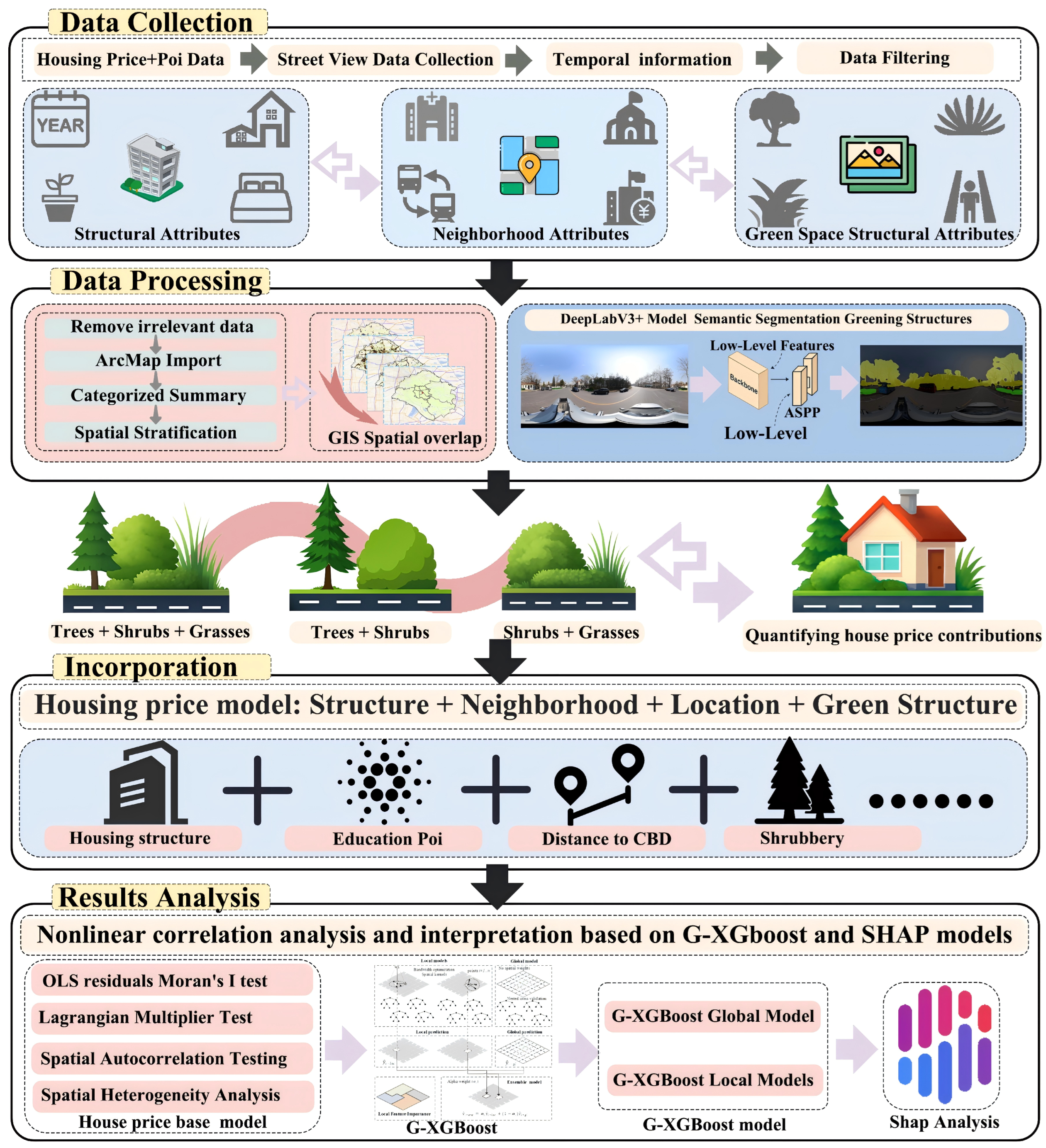
Disclaimer/Publisher’s Note: The statements, opinions and data contained in all publications are solely those of the individual author(s) and contributor(s) and not of MDPI and/or the editor(s). MDPI and/or the editor(s) disclaim responsibility for any injury to people or property resulting from any ideas, methods, instructions or products referred to in the content.

Article Metrics

Citations

Article Access Statistics

Multiple requests from the same IP address are counted as one view.