Spatial and Efficient Channel Attention for Multi-Scale Smoke Detection

Abstract

Attention mechanism-based deep learning has played an important role in vision-based smoke detection in forest fire early warning systems. However, the lack of consideration of the specific characteristics of smoke may render existing attention mechanisms ineffective, e.g., in detecting small areas of smoke, particularly in the complex forest smoke scenes involving multiple points of ignition or varying scales. To enhance the accuracy and the interpretability of smoke detection, we propose a Spatial and Efficient Channel Attention mechanism, termed SECA, and integrate SECA into deep models to incorporate the characteristics of smoke diffusion. Technically, multi-kernel 1-dimensional (1D) convolution is utilized for multi-scale smoke-capturing, to replace single-kernel 2D or 3D convolution in existing methods. In implementation, our SECA mechanism can also be used as a common module and easily plugged into a backbone network. To accelerate our model, a DSConv-Haar Wavelet Downsampling technique called DHWD is also provided. Extensive experiments were conducted on public datasets and self-collected datasets. Compared to existing methods, our method can achieve a better or at least a comparable performance in smoke detection in terms of smoke detection accuracy, computational efficiency, and ease of use. For example, it surpasses baseline methods, demonstrating average improvements of 4.2% in mAP₅₀ and of 3.7% in mAP_50-95, respectively.

1. Introduction

Forest fire is one of the most serious threats to forest resources, ecosystems, and human society. In recent years, the rise in human activities, coupled with the deteriorating global environment, has greatly contributed to an increase in forest fire incidents [1]. Due to its large-area coverage, all-weather operation, low cost, and especially its ability to monitor accidental fires caused by human behaviors, vision-based fire and smoke detection techniques have been increasingly predominant in forest surveillance systems [2,3]. In this work, our primary focus is on smoke detection rather than fire detection, because smoke is usually viewed as an earlier sign of a fire incident.

In the literature, existing smoke detection methods can be roughly divided into three types: (1) classification of video frames, image blocks, or pixels into a smoke class or non-smoke class, (2) estimating bounding boxes of smoke objects in an image for smoke localization and detection, and (3) image region segmentation of smoke objects [4]. For these three types, supervised learning is a fundamental component, applied in smoke detection, recognition, localization, and segmentation. In the mode of machine learning, earlier smoke detection was supervised and can be traced back to Gubbi’s work [5], where both classes of samples were manually featured as 60-dimensional vectors, obtained from three-level wavelet decomposition on 32 $\times$ 32 image blocks. Then, a Support Vector Machine (SVM) was trained to classify these samples into two classes: smoke and non-smoke. From then on, the focus of smoke detection was on both directions: feature construction and model selection. In general, a smoke detection task commonly consists of three steps [6]. First, smoke features are constructed on smoke images or video frames to form vector-pattern samples. Second, a shallow learning model, such as SVM, AdaBoost, or random forest, is selected and trained on the featured samples. Finally, an unseen sample is identified by the trained model. For the shallow learning models, the main shortcomings lie in two aspects. One shortcoming concerns feature construction. The needed features are usually hand designed, heavily relying on the prior knowledge of the feature designer. Moreover, this over-reliance may exhibit poor scalability for smoke detectors. The other shortcoming refers to the limited representation capacity of shallow models. For example, shallow learning may be effective for a small dataset, owing to the handcrafted features, while on a large dataset, handcrafted features may fail to characterize the intricate characteristics of smoke due to the limited representation ability. To alleviate these issues, various deep models were later introduced into smoke detection. For example, Luo et al. [7] proposed a convolutional neural network (CNN)-based smoke detector, where suspected smoke regions were first detected, and then the features of these regions could be extracted automatically by this CNN. To integrate feature extraction, candidate box extraction, and classification, Cheng [8] introduced a fast R-CNN (Regional CNN) for smoke image recognition. Compared to the shallow learning model, both deep methods can improve the accuracy rate of smoke video detection. Additionally, considering the transparency characteristics of smoke, Zhan et al. [9] designed a variant ResNet (Residual Network) named ARGNet, in which two identical ResNet50-vd models were used for feature extraction. Specifically, high-level features were extracted by the first ResNet50-vd and transmitted to the second ResNet50-vd. Then, together with the low-level features extracted by the second ResNet50-vd, ARGNet was designed to enhance the ability to represent smoke, e.g., to capture the transparency of smoke objects. Experimental results on the constructed dataset named UAV-IoT (Unmanned Aerial Vehicle–Internet of Things) demonstrated that ARGNet had achieved a higher accuracy rate in UAV aerial forest fire smoke detection, as well as in identifying smoke-like objects, long-distance smoke, and the performance on the smoke positioning in complex smoke scenarios. In contrast, a deep network model is superior to the shallow one. One explanation is that the deep model has more powerful capabilities in semantic feature extraction. Here, semantic information typically encompasses low-level features such as the color, texture, or position of a smoke object, as well as high-level features like semantic fragment, contour, or smoke-object region [10]. Thanks to their powerful computation capacity in handling vast amounts of data, deep networks and their related variants, including lightweight versions [11,12,13], have achieved great success in smoke detection. Here we only name a few.

On the other hand, due to the black-box nature of complex network architecture, deep networks usually lack interpretability [14]. In this view, the attention mechanism provides a means to interpret the opaque behavior of neural architectures, which is valuable for vision-based tasks such as smoke detection [15,16]. Because the concept of saliency is more consistent with the visual attention mechanism of human beings, a salient smoke detection method in shallow learning was proposed in Ref. [17]. Although this method can detect most of the instances of smoke, it also achieves a high error warning rate. In the direction of smoke attention, most methods adhered to the paradigm of deep learning in the literature. To clarify, here we give some examples. In Ba et al.’s work, a model named SmokeNet [18] was proposed to enhance feature representation for smoke objects appearing in satellite imagery, by combining both spatial and channel information. However, it can be viewed as a failure, because SmokeNet was still prone to excessive error warnings. To reduce error warnings, He et al. [19] introduced another attention-based CNN model and attempted to identify smoke from a fog environment, where a lightweight feature-level and decision-level fusion was used to improve the identification of smoke, fog, and other objects. On the other hand, self-attention is another common mechanism in smoke detection. There have been multiple versions proposed for different purposes. For example, Jiang et al. [20] designed a Self-Attention Network for Smoke Detection named SAN-SD and applied it in industrial settings to detect smoke from low-resolution images where smoke was produced by straw burning. Considering transparency and variability, Wang et al. [21] advised a self-attention-based YOLO model named SASC-YOLO, where the self-attention mechanism is intended to emphasize smoke features, but its performance was evaluated on synthetic smoke datasets. Additionally, Wang et al. proposed a Multi-level Feature Fusion Network (MFFNet) [22], where the module named Attention Feature Enhancement was used to refine multi-scale features. However, this network was specifically utilized for smoke-screening satellite remote sensing images. In summary, these methods may be efficient in their individual scenarios; however, they cannot be used directly for our forest smoke detection concerns for the following reasons: (1) The used-attention mechanism is just a simple application of computer vision algorithms, with little or even no consideration of the characteristics of smoke. (2) They may be efficient for a simple scenario, e.g., one in which a single and large-scale smoke object appears. However, they will fail to detect complex smoke objects, e.g., smoke from a complex forest involving multiple points of ignition or varying scales.

In this work, our ambition is to propose a novel interpretable attention mechanism for multi-scale smoke detection. We highlight our contributions as follows.

(1)

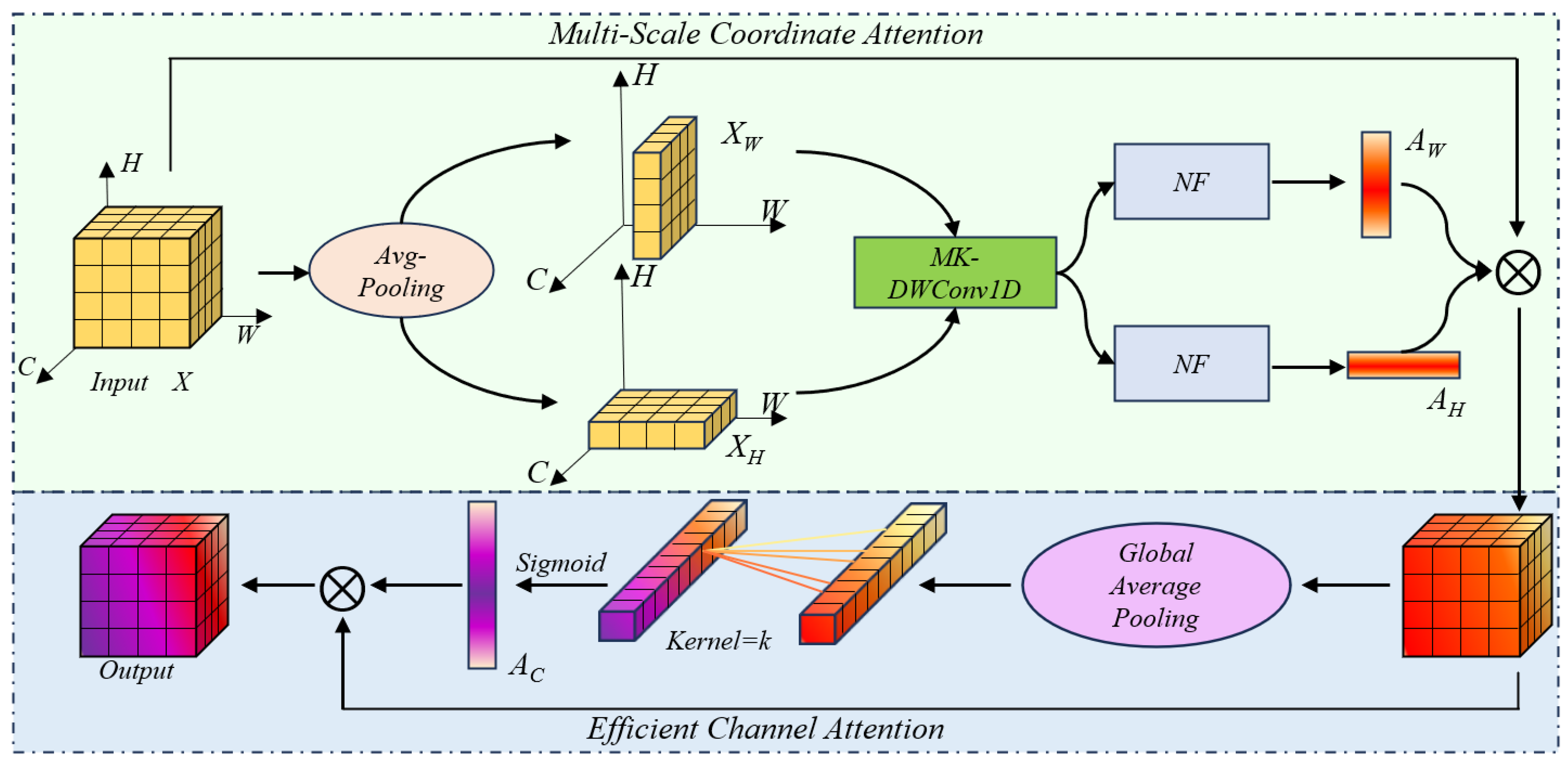
We propose a novel attention mechanism called Spatial and Efficient Channel Attention, abbreviated as SECA, for forest smoke detection.

(2)

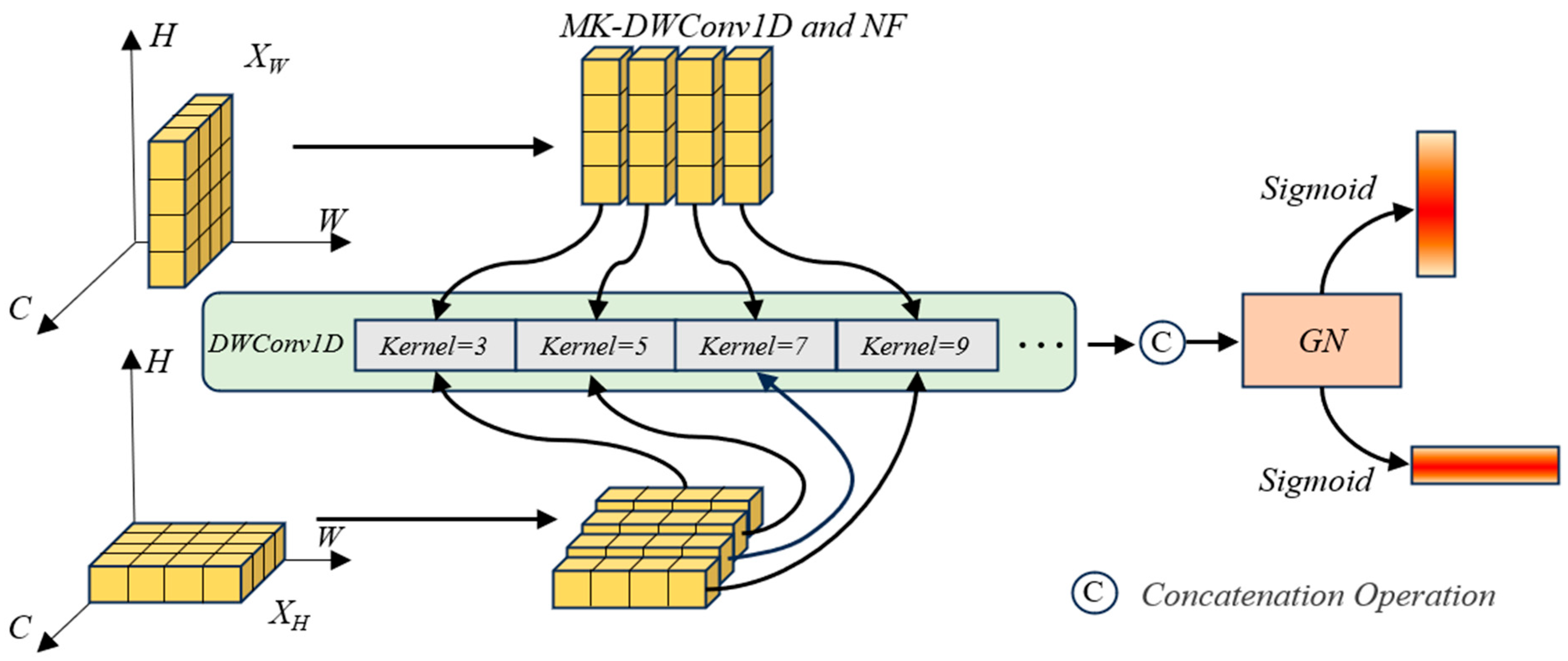
To improve the accuracy of multi-scale smoke detection, we construct feature maps via multi-kernel one-dimensional (1D) convolutions rather than single-kernel 2D or 3D convolutions in existing methods.

(3)

For interpretability, the channel features, also generated from 1D convolutions, can be explained as the weights to emphasize the importance of spatial features along the channel direction.

(4)

In terms of ease of use, our SECA can be used either as two isolated modules or as a unified module, and it can be easily plugged into a base network for smoke detection.

(5)

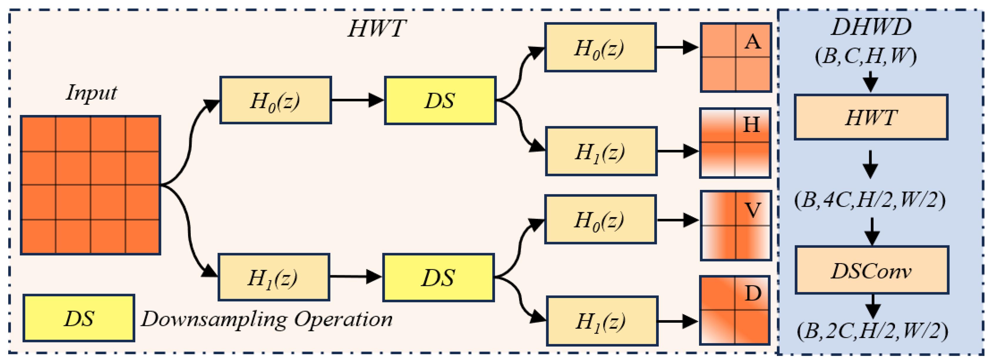
We also provide an acceleration strategy for model training, e.g., by leveraging a DSConv-Haar Wavelet Downsampling technique.

The remaining structure of this paper is organized as follows. In Section 2, we review some works that are the most related to ours. In Section 3, we detail our SECA mechanism, the resulting network, and the aforementioned acceleration strategy. Section 4 is dedicated to an extensive experimental evaluation, wherein a comparative analysis is conducted between our method and the state-of-the-art (SOTA) methods. Finally, we draw a conclusion in Section 5.

2. Related Work

This section briefly reviews the related work on smoke feature extraction. To clarify, it is divided into three subsections: traditional shallow feature extraction, spatial and channel attention mechanisms, and hybrid attention mechanisms.

2.1. Shallow Saliency

Treating smoke detection as a saliency detection problem is a prevalent approach in shallow learning, e.g., as seen in Jia’s work [17]. Inspired by the attention mechanism of the human visual system, Jia et al. considered the characteristics of smoke on two dimensions: color features and motion features. In terms of color features, the authors enhanced the color representation of smoke by analyzing the brightness changes. As for the motion features, they introduced optical flow motion analysis to capture the diffusion characteristics of dynamic smoke. By combining these two features, saliency maps of different dimensions were then calculated. Subsequently, the Bayesian estimation and the Otsu algorithm were employed to identify smoke and conduct pixel-level segmentation. This method has two limitations: (1) The computational efficiency of this method was found to be low, e.g., ten or more seconds per image for smoke detection processing; (2) The smoke identification was determined by a fixed threshold, which may limit its adaptability to environmental changes.

2.2. Spatial and Channel Attention Mechanisms

Channel attention and spatial attention represent two fundamental forms of attention mechanisms. On one hand, as discussed in Ref. [23], the first attention mechanism typically targets object-level features, while the second, in contrast, focuses on pixel-level semantic details. On the other hand, some experimental results have concluded that integrating attention into mainstream networks can enhance the ability of the model to understand fine-grained features [16]. As for the existing methods, Ba et al. [18] introduced a channel attention mechanism into smoke detection, where SENet (Squeeze-and-Excitation Network) [24] was leveraged for channel-wise feature recalibration to enhance discriminative channels. Through squeeze-excitation operations, the smoke features in the channel direction (e.g., color, texture) were adaptively emphasized, thereby effectively mitigating false positives, e.g., caused by smoke-like background objects. To enhance spatial localization, they cascaded a spatial attention module after the SE block and subsequent Fully Connected (FC) layers. However, the FC layers may generate computational redundancy and thus result in an insufficiency of spatial modeling capability [25]. Furthermore, they may also lead to suboptimal solution to multi-scale smoke identification. To mitigate this limitation, He et al. [19] suggested a spatial-channel co-attention framework in which 3 × 3 convolutions are employed to generate spatial weights alongside a SENet-inspired channel attention. Nonetheless, the fixed-sized convolutional kernels may be insufficient to capture the wide variations in complex forest smoke scenes.

2.3. Hybrid Attention Mechanisms

To capture the multi-scale nature of smoke, such as the varying shapes and scales of smoke objects, researchers have developed various attention-based hybrid architectures. For example, Wang et al. [21] adapted CBAM (Convolutional Block Attention Module [26]) for smoke detection. In contrast, CBAM presented an extension of SENet and constructed a dual-branch architecture by combining average pooling and max pooling to enhance local salient features in dense smoke regions. However, since smoke morphology can range from fine details to widespread dispersion in a real scene, conventional spatial attention mechanisms may struggle to represent this entire continuum. Likewise, Jiang et al. [20] proposed a multi-branch design for the GA-Block, expanding its architecture to a triple-branch framework inspired by Query-Key-Value interactions in self-attention mechanisms. The GA-Block may be effective in suppressing background-induced false positives. However, the intrinsic relationship between smoke characteristics and the triplet (Query-Key-Value) in self-attention appears to remain a question that requires further explanation. Another direction for the hybrid attention mechanisms, e.g., multi-scale feature fusion, has also been considered in smoke detection. It aimed to integrate hierarchical feature maps for robust smoke appearance and semantic learning. For example, in MFFNet [22], the module AFEM employed dual-path hierarchical attention, called local texture and global distribution, respectively, to fuse multi-scale features, which was combined with SENet for channel recalibration. Obviously, this method necessitates complex post-processing architectures and thus may affect the generalization of the model.

In summary, for the current attention mechanisms used in smoke detection, the main issues are threefold: (1) If compared to channel attention, spatial information is paid less attention, along with the directional or positional information of smoke objects; (2) For some attention mechanism-based methods, e.g., self-attention, it is hard to interpret why they are efficient for smoke detection. For example, until now it is still unclear which concepts in smoke detection can be explained as or correspond to Query (Q), Key (K), or Value (V), because these concepts originate from natural language processing and machine translation. (3) Both receptive fields and filter kernels for the convolutions are commonly fixed, and as a result they may fail in capturing multi-scale objects that appear at different sizes. In order to mitigate these issues, we propose the SECA mechanism and use it as a plug-and-play module in a deep network architecture. We also provide an acceleration strategy inspired by the lightweight design philosophy of CBAM [26] and CPCA (channel prior convolutional attention) [25].

3. Materials and Methods

In this section, we will detail our SECA mechanism. For easy interpretation, it can be decomposed into two parts, namely, Multi-Scale Coordinate Attention (MSCA) and Efficient Channel Attention (ECA), where MSCA is expected to focus on the position information of some important and distinct smoke objects, while ECA is expected to pay more attention to the object details.

3.1. SECA Mechanism

In practical situations, it is difficult to perform multi-scale smoke detection, due to the variability and rapid diffusion of smoke. For example, in a specified forest-monitoring spot, there may be multiple ignition points or different scales of smoke objects appearing in a diffused form, columnar form, or even both. We expect that our SECA can capture these smoke plumes. To clarify, we illustrate our SECA in Figure 1.

Figure 1. The flowchart of our SECA mechanisms.

We explain Figure 1 as follows. Let $X$ be an input tensor at the size of $C\times H\times W$, where $C$ denotes the number of channels, while $H$ and $W$ denote the height and width of $X$, respectively. Then $X$ is spatially decomposed into two sub-tensors, e.g., $X_H$ and $X_W$, along both the height and width directions. For this spatial decomposition, we employ it to extract smoke features when the smoke spreads out. Next, on each sub-tensor, we consider an operation called multi-kernel convolution, i.e., “MK-DWConv1D” in Figure 1, to capture the diffused smoke. In this case, the obtained height- and width-directional attention maps are denoted by $A_H$ and $A_W$, respectively. As for the efficient channel attention (ECA), shown at the bottom of Figure 1, it is used to assign attention weights to individual channels, aiming to selectively emphasize which features are more relevant to smoke detection. In the ECA step, an adaptive kernel operation shown in “Kernel = k” in Figure 1 is also considered. For convenience, we use $A_C$ to denote the attention map of ECA. In computation, after both the MSCA and ECA mechanisms are sequentially executed, the final output can be preserved in the same dimension as the input tensor $X$. In the next subsections, we will describe more details, including the implementation of the above steps.

3.1.1. Multi-Scale Coordinate Attention

As mentioned above, in the Multi-Scale Coordinate Attention (MSCA) step, we perform spatial decomposition to form two direction-specific sub-tensors: one is along the height (H) direction, and the other is along the width (W) direction. The two obtained components are represented as X_H (∈ ℝ^C×1×W) and X_W (∈ ℝ^C×H×1) in Figure 1. Then we repeat the decomposition on the decomposed components, aiming to capture finer-grained features from multiple scales of the diffused smoke. In this case, we name these fine-grained components as segment-components hereafter. In this work, we empirically decompose both sub-tensors into eight segment-components, defined in Equations (1) and (2).

$$X_H^i=X_H[(i-1)\times {\displaystyle \frac{C}{4}}:i\times {\displaystyle \frac{C}{4}}, : , :],\hspace{1em}i=1 \mathrm{to} 4,$$

(1)

$$X_W^i=X_W[(i-1)\times {\displaystyle \frac{C}{4}}:i\times {\displaystyle \frac{C}{4}}, : , :],\hspace{1em}i=1 \mathrm{to} 4,$$

(2)

where C and i denote the channel dimension and the index for the segmented components, respectively. Here, both components, either in the height- or in the width-direction, are decomposed into the same number of segments, to maintain consistency with the computations in the next steps. The advantages are twofold: (1) Such decomposition can provide a more flexible representation, e.g., for the above-mentioned multi-scale or cross-scale smoke objects; (2) It may have more potential in smoke-capturing. Some evidence in the literature has indicated that leveraging multi-scale receptive fields may allow a network to capture multi-scale or across-scale features [27,28].

After segment-component decomposition via Equations (1) and (2), the obtained segments are then fed into depthwise 1-dimensional (1D) convolutions in parallel, together with expanding kernel sizes, e.g., at the sizes of K = 3, 5, 7, and 9, respectively. We name these convolutions Multi-Kernel Depthwise Conv1D, i.e., MK-DWConv1D for short. This process can be represented by Equation (3):

$${\hat{X}}_k^i=\mathrm{MK}-\mathrm{DWConv}1\mathrm{D}(X_k^i),\hspace{1em}\hspace{1em}k\in \{H,W\}, i=1 \mathrm{to} 4.$$

(3)

In Equation (3), the so-called MK-DWConv1D is defined in Equation (4),

$$\mathrm{DWConv}1\mathrm{D}(X_n^i,l)=(X_n^i*K)(l)={\displaystyle {\sum }_{m=0}^M{X}_n^i(l+m)\cdot K(m)},$$

(4)

where both symbols $X_n^i$ (1D array of the length $n/4$) and $K$ (1D array of depth $M$) denote the input and the kernel; the operator “*” means the 1D convolution between $X_n^i$ and $K$, operated at the position of $l$. We expect that, when varying $l$ along the direction of $X_n^i$ and also varying the kernel size of $K$, 1D convolution can provide a greater potential in capturing different scales of smoke objects, especially for those objects also diffused along this direction, compared to 2D or 3D convolutions.

Naturally, in contrast to single-kernel, multi-kernel means multiple receptive fields are used for capturing different scales of smoke objects. We expect that such a design enables layered feature abstraction. For example, we expect that smaller kernels can capture more details, e.g., high-frequency patterns and local patterns essential for edge detection, such as the distinct boundaries of dense smoke particles closer to ignition points. We also expect that larger kernels can model long-range contextual dependencies and can capture the broad dispersion patterns of the diffused smoke. As for the intermediate-scale kernels, we expect them to bridge these extremes, facilitating a smooth transition across spatial scales and thereby allowing for the capture of evolving smoke characteristics from source to diffusion. The implementation of the MK-DWConv1D is shown in Figure 2.

Figure 2. The illustration for spatial attention feature map generation.

Figure 1 also illustrates both operations, called Normalization and Fusion (NF); they both are considered for the subsequent data processing. Correspondingly, the Group Normalization (GN) in Figure 2 is expected to capture dynamic intensity variations characteristic of smoke objects. For example, the channel-wise standardization for GN is expected to preserve inter-channel independence and thus to attain detailed characteristics of smoke. To approach this goal, the Sigmoid is selected as an activation function for the GN operation, and 0–1 binary outputs are used to distinguish smoke objects from non-smoke ones. In implementation details, the attention maps, denoted by $A_w$ and $A_H$ in Figure 1, can be calculated by the following equations,

$$A_H=\sigma \left(G{N}_H\left(Concat\left({\widehat{X}}_H^1,{\widehat{X}}_H^2,{\widehat{X}}_H^3,{\widehat{X}}_H^4\right)\right)\right),$$

(5)

$$A_W=\sigma \left(G{N}_W\left(Concat\left({\widehat{X}}_W^1,{\widehat{X}}_W^2,{\widehat{X}}_W^3,{\widehat{X}}_W^4\right)\right)\right),$$

(6)

where $\sigma (\cdot )$ represents the Sigmoid function and $G{N}_H(\cdot )$ and $G{N}_W(\cdot )$ represent GN operations on their own dimensions. We use ${\widehat{X}}_H^i$ and ${\widehat{X}}_W^i$ to denote the outputs of MK-DWConv1D operations on the i-th segment-component in both H and W directions, respectively. Then, the concatenation operator, denoted by $Concat(\cdot ,\dots ,\cdot )$, is applied to the convolution outputs of segment components. Finally, our final feature map in MSCA can be computed by Equation (7),

$$MSCA(X)=X\times A_H\times A_W.$$

(7)

3.1.2. Efficient Channel Attention

In order to utilize channel information, we also develop a module named Efficient Channel Attention (ECA) for smoke detection, aiming to capture inter-channel dependencies of smoke objects. Similar to MSCA, we also expect that our ECA can help our SECA to reduce computational workload, as addressed in Ref. [29]. As depicted in Figure 1, the MSCA output (attention map), i.e., $MSCA(X)$, can also be viewed as a new input for the ECA module, because its size is the same as the original input $X$. That is, they all share the same size of $C\times H\times W$. In this view, both our MSCA and ECA can be viewed as isolated modules for smoke detection, which provides a significant benefit in ease of use. Additionally, to show their individual performance, these two modules will be verified in the experiment section. In computation, we also simplify the ECA input as 1D tensors and let all the 1D tensors share the same size, e.g., at the size of $C\times 1\times 1$. Intuitively, our proposed 1D decomposition will be beneficial for subsequent parallel computing. To approach this goal, we use global average pooling (GAP, for short) on every 2D tensor, i.e., the sub-tensor of $MSCA(X)$ obtained by 2D decomposition along the channel direction. Then, the 1D convolution with a size-adaptive kernel, i.e., “Kernel = k” in Figure 1, is applied to every channel-wise 1D tensor. For the kernel size k, we follow Ref. [29] and define it in Equation (8),

$$k={⌊{\displaystyle \frac{{\log }_2(C)}{\gamma }}+\beta ⌋}_{odd},$$

(8)

where parameters $\gamma$ and $\beta$ denote the empirical scale factor and the offset of the convolution. This $C$ also refers to the total number of channel dimensions. The symbol ${⌊·⌋}_{odd}$ denotes an odd operator for a positive real value. After the above operations, the channel attention map for a given 1D tensor, denoted by $A_C$ in Figure 1, can be obtained. This map is then subsequently applied to recalibrate $MSCA(X)$ through channel-wise multiplication. As a result, the final output of ECA can be described by the expression ECA(X) = A_C $☉$MSCA(X), where the operator “$☉$” denotes element-wise dot product. In this case, $A_C$ can be explained as the weights to emphasize the importance of every spatial 2D tensor along the channel direction. This point will also be verified in Section 4.1. With the above-mentioned operations, for a given input $X$, our SECA can be expressed in a unified form. For simplicity, we write it in Equation (9),

$$SECA\left(X\right)=ECA\left(MSCA\left(X\right)\right).$$

(9)

We summarize the advantages as follows. Compared to the attention mechanisms applied in smoke detection, the proposed SECA is expected to extract finer-grained features in both spatial and channel directions. To capture the diffusivity of multi-scale forest smoke, we adopt multi-kernel convolutions on the decomposed 1D tensors, rather than single-kernel convolutions on 2D or 3D tensors as the existing methods do. Geometrically, our SECA can be viewed as two modules isolated from each other, or as a unified module defined in Equation (9), for ease of use and interpretability. Additionally, when working as an attention mechanism, SECA can be used as a standard module and plugged into a deep network for smoke detection. For the convenience of readers, we rename the resulting network as the SECA-XX network, where “XX” means the name of base network. This will be detailed in the next subsection.

3.2. SECA-YOLO Network

For simplicity, we use YOLOv8 as the backbone network and our SECA as a standard plug module, embedded in the given network. The architecture of the resulting network, called SECA-YOLO, is illustrated in Figure 3. A total of three SECA modules have been integrated into the P3, P4, or P5 stages of YOLOv8, respectively, with each module dedicated to processing features at a different scale. For example, we set the layers P3, P4, and P5 to the small, medium, and large scales of smoke objects, respectively. Thus, the final result of multi-scale smoke detection, as shown in the right panel of Figure 3, can be obtained by integrating all outputs of SECA.

Figure 3. The architecture of our SECA-YOLO network. A total of three SECA modules have been plugged into the backbone network, which are highlighted in red text in the middle panel. For reference, we also show the original architecture of YOLOv8 in the left panel. The final result of multi-scale smoke detection is shown in the right panel, where the outputs of SECAs are stacked together.

3.3. Acceleration Strategy

In the YOLO family, the downsampling operation is commonly performed by a standard strided convolution, e.g., with a kernel size of 3 and a stride of 2. For the complexity of a deep model, the parameter magnitude of standard convolutions is commonly determined by both the kernel size and the number of channels. Thus, the computational load, predominantly resulting from extensive multiply-accumulate operations, substantially adds to the overall computational burden. In order to reduce computational cost, in this work, we aim to replace traditional convolution-based downsampling with the Haar Wavelet Transformation (HWT). Ref. [30] stated that HWT can preserve critical local features and capture fine textures and edge details when input signals are decomposed into low- and high-frequency components.

To clarify, we illustrate HWT in Figure 4 and define the 1D Haar transformation in Equations (10) and (11),

$${\varphi }_0(x)=\left\{\begin{array}{cc}0\hspace{1em}\hfill & \hfill x<0\\ 1\hspace{1em}\hfill & \hfill 0\le x<1\\ 0\hspace{1em}\hfill & \hfill x\ge 1\end{array}\right.,$$

(10)

$$\left\{\begin{array}{c}{\varphi }_1(x)={\varphi }_0(2x)+{\varphi }_0(2x-1)\\ {\psi }_1(x)={\varphi }_0(2x)-{\varphi }_0(2x-1)\end{array}\right.,$$

(11)

where ${\varphi }_0(\cdot )$ and ${\varphi }_1(\cdot )$ are scaling functions at the 0–1 stage. ${\psi }_1(\cdot )$ denotes a wavelet basis function at Stage 1. Here, we let ${\varphi }_1(\cdot )$ correspond to the above-mentioned low-frequency information, which can be captured by a low-pass filter, denoted by $H_0$ in Figure 4. Likewise, $H_1$ in Figure 4 denotes a high-pass filter. $H_0$ corresponds to ${\psi }_1(\cdot )$ and is used to capture high-frequency information. Thus, for an input of size $C\times H\times W$, four wavelet components can be generated, namely, one low-frequency component (denoted by A) and three high-frequency components along horizontal (H), vertical (V), and diagonal (D) directions, respectively. At this time, each component has a size of $C\times (H/2)\times (W/2)$.

Figure 4. The structure for our DSConv-Haar Wavelet Downsampling (DHWD), where “DS” means a downsampling operation, while the “B” in (B, C, H, W) refers to batch size, e.g., the mini-batch of B inputs. The symbols “A”, “H”, “V”, and “D” represent different wavelet components.

Following HWT, the resulting four components are then concatenated along the channel direction to form a feature map, at the size of $4C\times (H/2)\times (W/2)$. Then Depthwise Separable Convolution (DSConv) [31], a standard convolution in DHWD, is used to produce a $2C\times (H/2)\times (W/2)$ output. It is worth noting that for the wavelet computation, all of the 1D convolutions can be achieved by a simpler addition or subtraction operation, rather than by more complex convolutions on 2D or 3D tensors, as they appeared in the related methods, though they have seldom been used in vision-based tasks. That is, if we replace the convolutions in the YOLOv8 backbone with our DHWD, both the computational cost and the number of parameters can be greatly reduced. For easy reading, we use Figure 5 to show this replacement, in which our downsampling module DHWD has been embedded into the backbone of YOLOv8.

Figure 5. The illustration of the DHWD embedding, where DHWD is highlighted by blue-background boxes. Compared to the backbone of YOLOv8, the original convolutions have been replaced with our DHWD to reduce computational workload.

3.4. Materials

In this subsection, the data used in this work will be briefly reviewed. It mainly consists of both collected smoke images and the smoke frames drawn from a forest smoke video. We organize these data into two datasets for different purposes. For example, one is used for multi-scale smoke detection, and the other is used for small and long-distance smoke detection. We address them as follows.

The first dataset, named FUAV (Fire data captured by Unmanned Aerial Vehicle), is made up of more than 1200 images, including smoke images and non-smoke ones. To avoid unbalanced learning, we set the number of samples in each class to be as equal as possible. FUAV has two main data sources. One is drawn from the source titled “Smoke Detection Based on Scene Parsing and Salient Segmentation”, available at http://smoke.ustc.edu.cn/. This source is composed of real forest fire images provided by the State Key Laboratory of Fire Science, University of Science and Technology in China. The other dataset is called FLAME, with the full name of Fire Luminosity Airborne-based Machine learning Evaluation, available at https://ieee-dataport.org/open-access/flame-dataset-aerial-imagery-pile-burn-detection-using-drones-uavs (accessed on 3 November 2025). This data source is from aerial imagery FLAME (Fire Luminosity Airborne-based Machine learning Evaluation) using drones located at the Ponderosa pine forest in Observatory Mesa in Northern Arizona, USA. This aerial pile burn detection database consists of different repositories. Among them, the first raw video recorded with the Zenmuse X4S camera was used for data preparation. In order to provide accurate supervision information for different scales of smoke objects, nearly 600 smoke images in FUAV have been well-annotated in a manual or semi-manual way. During this process, the tool LabelMe was also adopted for the smoke annotation, e.g., manually drawing bounding boxes around smoke or non-smoke regions, and then assigning them with Ground-Truth (GT) labels. In this work, the smoke data is labeled as positive, while the non-smoke data is labeled as negative. As for the performance assessment, the indicators in binary classification, such as true positive (TP), false positive (FP), false negative (FN), and intersection over union (IoU), can be used to measure the performance of smoke detectors. Here, the indicator IoU qualifies the spatial overlap between two bounding boxes, obtained by the GT and the predicted output of a trained network. Then the IoU value can be calculated by the ratio of the intersection area of both boxes to their union area. For smoke identification, the following analysis uses an IoU threshold of 0.5 as a standard reference. That is, for a true smoke image, if the obtained IoU value is greater than or equal to 0.5, this prediction is viewed as correct and can be labeled as positive; otherwise, it is incorrect. Furthermore, the value of prediction can also be used to compute TP and FP. For example, a valid predicted bounding box is recorded as TP if its prediction matches the GT. On the contrary, if it fails to meet the IoU threshold, e.g., the IoU value is less than 0.5 or has been assigned an incorrect label, the prediction will be recorded as FP.

The second dataset is called WSv2, titled “Wildfire Smoke dataset Version 2.0” and is available at https://github.com/aiformankind/wildfire-smoke-dataset (accessed on 3 November 2025). This dataset is provided by the AI Mankind team, located in San Jose, CA, USA. Both the fire and smoke images are captured by HPWREN cameras. For the image annotation, there are two versions, both using the Pascal VOC annotation format. In version 1.0, a total of 744 images annotated with bounding boxes were created; in version 2.0, a total of 2192 images for fire and smoke objects were annotated. In this work, we use it for a challenging smoke detection task, because some of the smoke objects are difficult to annotate, even by human vision.

4. Results

To evaluate the performance of our proposed attention mechanism SECA, we take YOLOv8 and YOLOv11 as base networks. All YOLO models are implemented in the PyTorch environment of Ultralytics. To show the comparison extensively, some state-of-the-art (SOTA) methods are used as baselines, which will be detailed in the following subsections. Our training epochs and batch size are set to 200 and 8, respectively, the recommended parameters for the YOLO-series networks in the literature. Other parameters are retained as the default values, e.g., those provided by the Ultralytics community. For the non-YOLO models, they are implemented in the Mmdetection3.0 environment, with the default values provided by Mmdetection3.0.

The composite indicators, such as Precision (P), Recall (R), mAP₅₀, and mAP_50-95 are also commonly used for performance assessment. For the convenience of readers, we list them as follows. They are defined as $\mathrm{P}$$=$$\mathrm{TP}/(\mathrm{TP}+\mathrm{FP})$, $\mathrm{R}$$=$$\mathrm{TP}/(\mathrm{TP}+\mathrm{FN})$, ${\mathrm{mAP}}_{50}$$=$${\displaystyle {\sum }_{i=1}^N{\mathrm{AP}}_i}/N$, and ${\mathrm{mAP}}_{50-95}=$$[{\displaystyle {\sum }_{i=1}^N({\displaystyle {\sum }_{j=1}^{10}{\mathrm{AP}}_{i,j}}/10)]}/N$, where $N$ denotes the total number of classes. For the AP, defined as $\mathrm{AP}={\displaystyle {\int }_0^1\mathrm{P}(\mathrm{R})d\left(\mathrm{R}\right)}$, it is the area under the Precision-Recall curve for a specific class. The indicator mAP₅₀ calculates the mean average precision at a single IoU threshold of 0.5 (the percentage value of 50), assessing detection performance under relatively loose localization. Likewise, mAP_50-95 provides a more comprehensive evaluation by averaging precision over 10 IoU thresholds, ranging from the percentage values of 50 to 95 (or 0.5 to 0.95 in real value) with a fixed step of 5 (0.05). We use it to assess the performance of multi-scale smoke detection, measured by IoU positioning accuracy, where ${\mathrm{AP}}_{i,j}$ is the $\mathrm{AP}$ value of the i-th class at the j-th IoU threshold. In practical situations, P is usually used as an indicator to measure the accuracy rate of smoke detection. For example, a high p-value means that the model may result in an accurate classification. Likewise, R indicates the model’s ability to prevent missing detections of smoke. A high R value means the network identifies most potential smoke regions, enabling its use in early fire alarms. Additionally, an F1-score, defined as ${\mathrm{F}}_1=\left(2\times \mathrm{P}\times \mathrm{R}\right)/(\mathrm{P}+\mathrm{R})$, is also used as a performance metric because it is also popular in vision-based smoke detection.

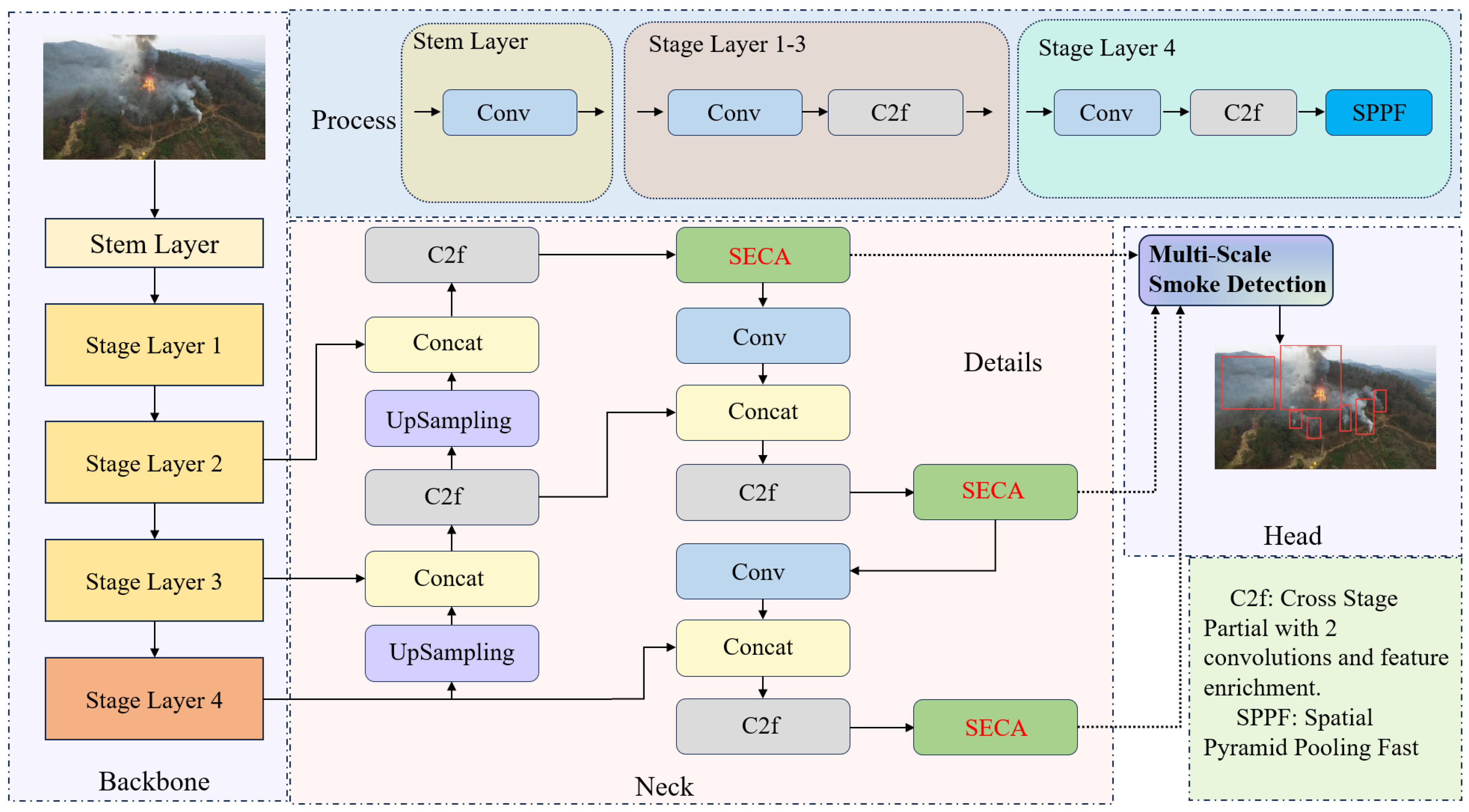
To show the comparison more clearly, we divide the experiment into two subsections. In the first subsection, an ablation experiment is carried on our SECA, which encompasses evaluating the contribution and interpretability of the proposed modules. In the second subsection, we compare our SECA with SOTA baselines. This comparison consists of two parts. The first part is to show the comparison between our SECA and multiple newly proposed SOTA attention modules, some of which may not be used for smoke detection. For fairness, these modules are embedded in the same positions that our SECA has been embedded in, as illustrated in Figure 3. In the second part, we compare our SECA-based YOLO networks, YOLO-SECA for short, with state-of-the-art smoke detectors. All experiments were conducted on a workstation equipped with an NVIDIA GeForce RTX 4060 GPU (8 GB VRAM) and an Intel^® Core™ i9-13900HX processor. The software environment consisted of Python 3.9, PyTorch 2.0.1, and CUDA 11.8, with code developed in Visual Studio Code (version 1.91.1).

4.1. Performance Assessment for Our SECA

In this subsection, we use an ablation experiment to evaluate the effectiveness of our proposed SECA, including the isolated modules of MSCA or ECA, the unified module of SECA, and the acceleration strategy DHWD. The results are listed in Table 1 and Table 2 and Figure 6, respectively.

Table 1. The results of the ablation experiment on the FUAV dataset.

Method	P (Precision)	R (Recall)	mAP50	mAP50-95	Parameter (MB)
YOLOv8 (Naive)	0.803	0.765	0.800	0.328	3.011
+MSCA	0.781	0.776	0.794	0.320	3.016
+ECA	0.817	0.735	0.798	0.328	3.011
+SECA	0.818 *	0.779	0.815	0.345	3.016
+DHWD	0.804	0.746	0.796	0.316	2.800
+SECA + DHWD	0.813	0.769	0.823	0.339	2.800

* Best results are shown in bold.

Table 2. The training speed comparison between our DHWD and standard convolutions (Conv).

Strategy	Training Time (s)	FLOPs (G)	Parameter (KB)
DHWD	36.4 *	9.261	71.04
Conv	95.3	77.578	147.12

* Best results are shown in bold.

Figure 6. Illustration for the heatmaps. For the given smoke images (a), we show the Grad-CAM heatmaps in (b–d), obtained by MSCA, ECA, and SECA, respectively. For better visualization, the regions for multi-scale smoke have been highlighted in orange boxes.

At first glance, Table 1 shows that in terms of the five indicators, the unified module YOLO-SECA performs the best, followed by YOLO-SECA-DHWD. For example, YOLO-SECA achieved the highest p-value of 0.818, the highest R of 0.779, and the highest mAP_50-95 value of 0.345. As for the other two indicators, it still achieves the second-best mAP₅₀ value of 0.815, which is just 0.008 points less than the best value of 0.823. In this case, because YOLO-SECA does not use the DHWD strategy, the magnitude of parameters in YOLO-SECA (indicator Parameter in Table 1) is slightly higher than that of the pure YOLOv8. On the contrary, if DHWD is considered, the value of the indicator Parameter is greatly reduced, e.g., from 3.016 MB to 2.8 MB. On the other hand, if an isolated module, MSCA or ECA, is considered, the resulting YOLOv8-based models may outperform the naive one, as shown in Table 1, where some of the indicator values in YOLO-MSCA and YOLO-ECA have surpassed those of the naive YOLOv8. Additionally, Table 1 also shows the effectiveness of the proposed acceleration strategy DHWD, where the Parameter values of models YOLO-DHWD and YOLO-SECA-DHWD have been reduced to 2.8 MB, compared to the value of 3.011 MB in the naive model. This point will be further verified in Table 2.

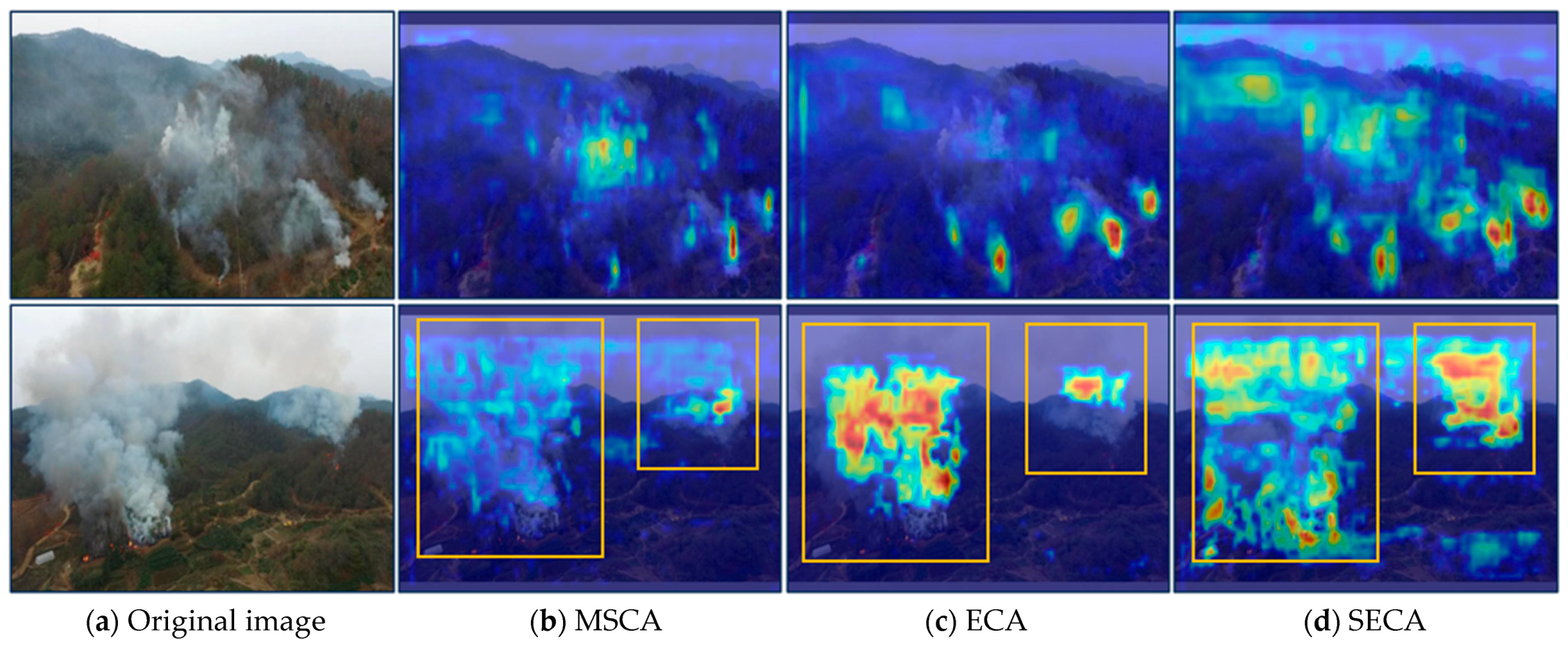
To show the accuracy of extracted features, for intuition, heatmaps of Grad-CAM (Gradient-weighted Class Activation Mapping [32]) are used in this work. This is because in computer vision, the Grad-CAM tool is popularly used in feature visualization. To display the performance on different scales, especially for the performance on multi-scale smoke detection, we prefer to visualize FUAV data by heatmaps. To clarify, limited by space, both images from FUAV data have been selected to represent multi-scale smoke, representing their heatmaps in Figure 6. As shown in Figure 6a, in each smoke image, there are multiple complex smoke objects, rather than one simple object appearing in the literature. For example, the so-called complexity here for the selected smoke objects is reflected in a variety of sizes and the diffusion in different directions, which is even beyond human vision; for example, it is difficult to know the accurate number of smoke regions. Correspondingly, we show the heatmaps in Figure 6b,d, provided by our attention modules MSCA, ECA, and SECA, respectively. For better visualization, we take the smoke objects in the second image as an example and highlight them in orange-colored boxes. If a heatmap is compared to the original image, it seems more intuitive to evaluate the accuracy of feature extraction. Following this intuition, it is evident that our SECA is superior to the other two attention modules. For example, a majority of smoke regions have been accentuated with brighter colors, while non-smoke regions appear in darker hues. On the one hand, it is observed that the heatmap from our SECA is not a straightforward superposition of the heatmaps from MSCA and ECA. This can be explained by the fact that, for example, the brighter smoke regions in MSCA or ECA heatmaps have not been displayed in the brighter regions of the SECA heatmap, and vice versa. On the other hand, the smoke location information captured by MSCA can be transmitted to SECA. For example, the blue smoke regions within the MSCA orange box exhibit a more vivid hue than the original blue and are more distinctly visualized in the SECA orange box. We explain it by using $SECA\left(X\right)=ECA\left(MSCA\left(X\right)\right)$ defined in Equation (9), where ECA(X) = A_C $☉$ MSCA(X). For the position feature $MSCA(X)$, the channel output $A_C$ has been used in SECA as weights, which is used to emphasize the importance of all of the obtained location features. As a result, both location information and channel information for smoke objects can be transferred to the final feature map. When Grad-CAM is applied for visualization, an important feature will be assigned a brighter color. In this view, this Figure can also be viewed as evidence for the interpretability of our SECA.

To provide a clear comparison for our acceleration strategy, DHWD, we take the standard convolutions (Conv) in YOLOv8 as a baseline and use training time (in seconds) for the performance assessment. For convenience, a total of 300 images were randomly selected from both datasets to establish a small training set. Then these training images were fed to the naive model and our YOLO-DHWD, where our DHWD was designed in accordance with the settings outlined in Figure 5. The size of input tensors of both models was unified to (8,128,256,256), for a fair comparison. After 30 warm-up iterations, we recorded training time in seconds, FLOPs in Giga, Parameters in KB, and listed them in Table 2. As a result, Table 2 shows that our DHWD significantly surpasses standard convolutional techniques, exhibiting a nearly threefold increase in speed when compared to the convolutions employed in the base model.

4.2. Comparison Between Our SECA and SOTA Baselines

As aforementioned, in this subsection, we aim to show the result in twofold, namely, to represent the comparison between attention mechanisms, and to provide a comparison between the selected state-of-the-art (SOTA) smoke detection models.

4.2.1. Comparison of Attention Mechanisms

In computer vision and vision-based applications, attention mechanisms have gained immense popularity. To show the novelty of our proposal, we take newly proposed attention mechanisms as baseline methods, including Efficient Multi-Scale Attention (EMA, in 2023) [33], Multi-scale Cross-axis Attention (MCA, in 2023) [34], Channel Prior Convolutional Attention (CPCA, in 2024) [25], and Global-to-Local Spatial Aggregation (GLSA, in 2024) [35], though some of them may not have been applied for smoke detection. Here, we should point out that we do not take the classic Coordinate Attention (CA, 2018) [27] and Convolutional Block Attention Module (CBAM, 2021) [26] as baselines. The reason is that, for example, both EMA and CPCA can be viewed as new versions of CA or CBAM. Furthermore, the baseline attention mechanisms seem to have stronger performance in capturing multi-scale objects. For example, MCA is designed to utilize multi-scale features and long-range dependencies to capture the changes and morphology of interesting objects. While for GLSA, the authors claimed that it can utilize global and local spatial information for small object detection. Considering the similarity between these relevant objects and our concerned smoke, we are also interested in investigating the efficacy of these baselines in smoke detection. For fairness, the above-mentioned baseline attention mechanisms are all used as plug-and-play modules to replace our SECAs, similar to the way of the SECA network shown in Figure 3. To evaluate multi-scale smoke detection performance, we calculate five metrics on both the FUAV and WSv2 datasets. The FUAV dataset is assessed across multiple scales, while the WSv2 dataset is assessed on small-area, long-distance, and combined smoke scales. The quantitative and visual results are presented in Table 3 and Figure 7, respectively.

Table 3. The comparison between our SECA and SOTA attention mechanisms.

		FUAV				WSv2
Model	Parameter (MB)	mAP50	P	R	F1	mAP50	P	R	F1
YOLOv8	3.011 *	0.800	0.803	0.765	0.785	0.693	0.762	0.619	0.683
+EMA [33], (2023)	3.011	0.809	0.791	0.787	0.788	0.694	0.784	0.619	0.692
+MCA [34], (2023)	3.136	0.799	0.812	0.752	0.781	0.698	0.754	0.658	0.702
+CPCA [25], (2024)	3.190	0.794	0.799	0.768	0.783	0.686	0.788	0.625	0.697
+GLSA [35], (2024)	4.026	0.787	0.817	0.743	0.779	0.679	0.752	0.612	0.675
+SECA (Ours)	3.016	0.815	0.818	0.779	0.798	0.704	0.778	0.650	0.708

* Best results are shown in bold.

Figure 7. Visualization for smoke detection on WSv2 data. Panel (a) shows the original image and the annotation for smoke objects by using a red box. From Panels (b–f), they are smoke detection results, provided by SECA-, MCA-, GLSA-, EMA-, and CPCA-based YOLOv8 models, where a smoke region is highlighted in a red box if it has been detected.

Table 3 indicates that, at first glance, our SECA is still superior to other attention mechanisms, e.g., most indicators having been shown in bold. Especially on the data FUAV, three out of the four indicators for smoke detection have achieved the best results, highlighted in bold in the table. For example, our SECA has achieved the highest mAP₅₀ value of 0.815, the highest P (Precision) value of 0.818, and the highest F1-score of 0.798. Even on the indicator R (Recall), it still achieves the second best, i.e., the R value of 0.779, which is just 0.008 points less than that of EMA-attention. 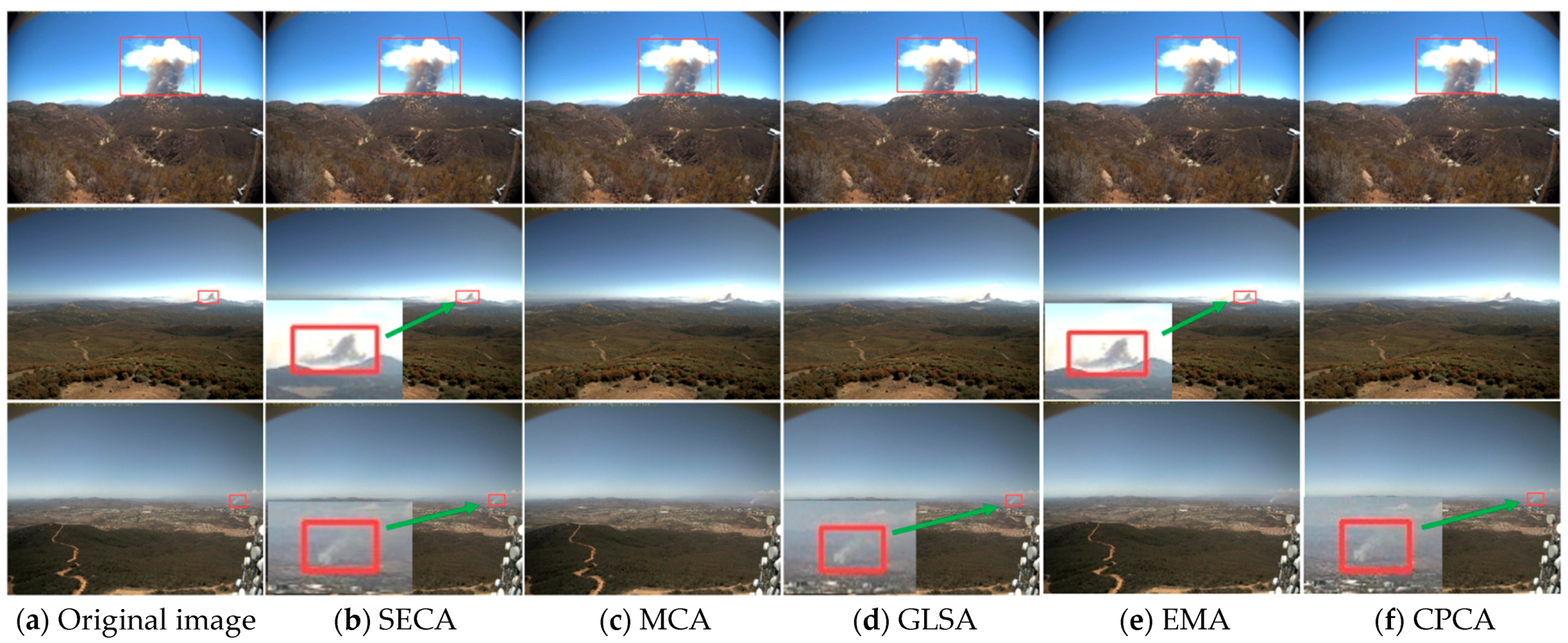Similarly, on WSv2, two out of the four indicators for SECA have also reached the highest levels, i.e., achieving an mAP₅₀ of 0.704 and an F1-score of 0.708. On the other two indicators, our SECA achieves a P value of 0.778 and an R value of 0.650, which are merely 0.01 and 0.008 points less than the best values obtained by CPCA and MCA attention, respectively. The reason may be attributed to two factors. (1) Our SECA has a stronger interpretability, e.g., capturing the diffusivity of smoke objects in both spatial directions of height and width. (2) For our adopted multi-kernel 1D convolution (MK-DWConv1D), it may have more potential in capturing different scales than single-kernel 2D or 3D convolutions applied in baseline attentions. To clarify, some challenging smoke objects are used for testing. Also, we visualize the detected results in Figure 7 for intuition.

In Figure 7, three selected smoke images from WSv2 data were used for visualization. For each image, the smoke object highlighted in a red box in Figure 7a was notably more complex, in terms of the spatial characteristics such as the size, orientation, and proximity to the observer in comparison to the smoke objects presented in FUAV data. The detection results are shown in Figure 7b,f, captured by SECA-, MCA-, GLSA-, EMA-, and CPCA-attention. To improve visualization, if a smoke object was correctly detected, a red box was added to the object to highlight the detection. As for the performance, the columnar smoke object in the first image could be captured by all attention-based methods. However, for the remaining smoke objects in the other two images, perhaps due to the smaller area in the monitoring fields, they sometimes failed to be captured by the baseline methods. For example, the smoke in the second image was missed by MCA, GLSA, and CPCA. Similarly, the smoke in the third image was missed by MCA and EMA. With regard to our SECA, Figure 7 shows that all of these challenging smoke objects could be correctly detected. The main reason for this phenomenon should still be attributed to our targeted design, i.e., using multi-kernel 1D convolutions to capture the diffusivity of smoke.

4.2.2. Comparison Among Different Networks

To provide a more extensive experiment, in this subsection, we aim to compare our method with SOTA mainstream models such as Faster R-CNN [36], Mask R-CNN [37], RetinaNet [38], TOOD [39] (Task-aligned One-stage Object Detection), DAB-DETR [40] (Dynamic Anchor Boxes-DETR), and RTMDet-Tiny [41] (Real-Time Models for Object Detection). Here, we have listed the original papers in our references to show our respect towards these authors and also to provide readers with a way to download the free codes if necessary. Among these models, most have been widely applied in fire or smoke detection [42,43]. To show the extensibility, both YOLO versions, e.g., YOLOv8 and the newly proposed YOLOv11, are used as backbones for our YOLO-SECA. 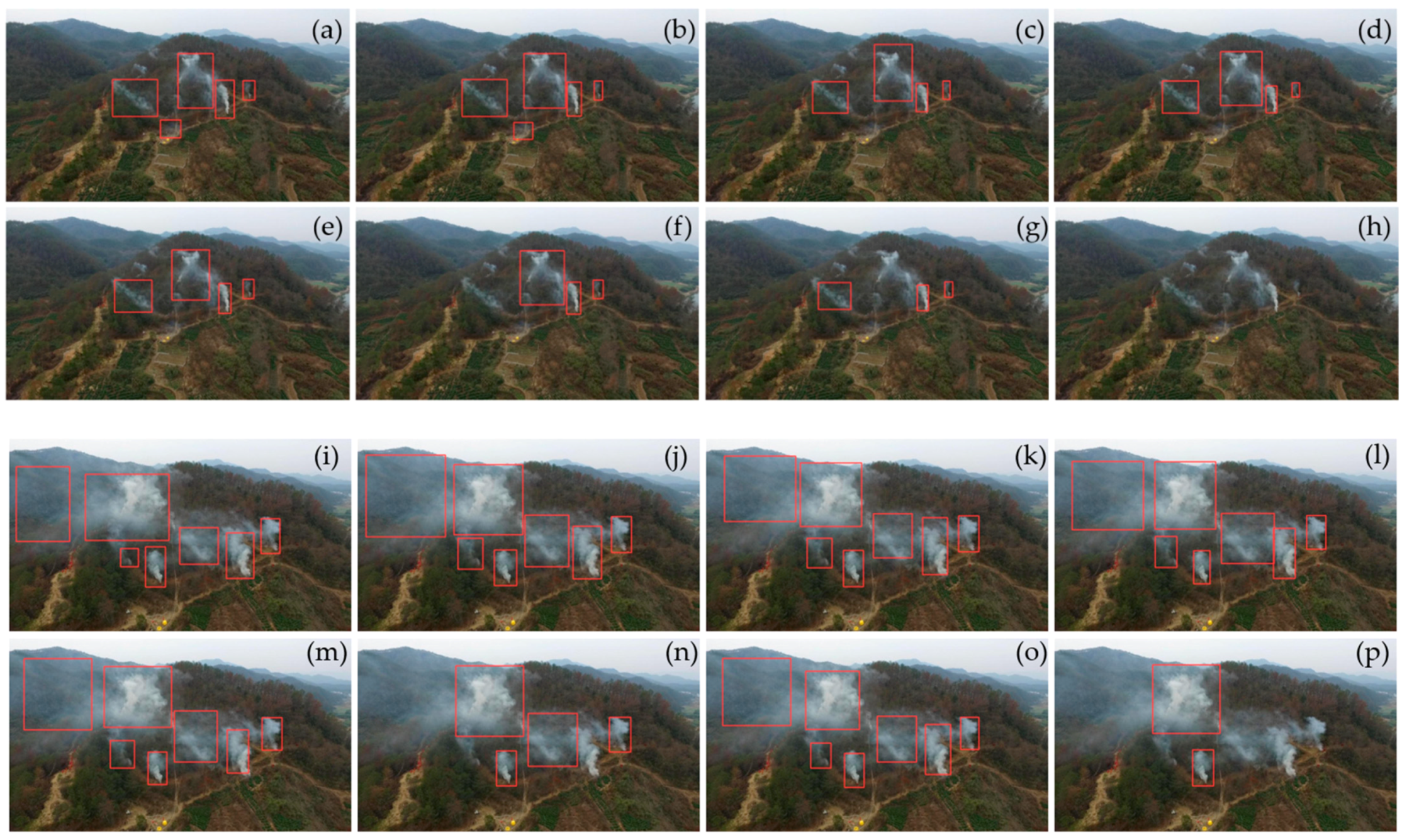We show the numerical value results in Table 4 and visualizations for multi-scale smoke detection in Figure 8.

Table 4. The comparison between different networks for smoke detection.

Model	mAP50	mAP50-95	FLOPs (G)	Parameter (MB)	Latency (ms)
Faster R-CNN [36]	0.760	0.311	208.0	41.348	144.9
Mask R-CNN [37]	0.779	0.317	261.0	43.991	74.6
RetinaNet [38]	0.795	0.320	155.0	19.771	37.0
TOOD [39]	0.760	0.289	199.0	32.018	71.9
DAB-DETR [40]	0.765	0.277	102.0	43.702	49.8
RTMDet-Tiny [41]	0.744	0.261	8.0	4.873	13.2
YOLOv11 [44]	0.780	0.312	6.4	2.590	7.6 *
Average results	0.769	0.298	134.2	26.899	57.0
YOLOv8 + SECA (Ours)	0.815	0.345	8.2	3.016	8.6
YOLOv8 + SECA + DHWD (Ours)	0.823	0.339	7.6	2.800	8.3
YOLOv11 + SECA + DHWD (Ours)	0.794	0.322	6.1	2.327	7.9
Average results (Ours)	0.811 #	0.335	7.3	2.714	8.3

* Best results are highlighted in bold, with a comparison between the different models. # Italics indicate the average of baseline results and our results, and the best result between the two is denoted by bold and underlining.

Figure 8. Visualized comparison among different models, where two images and the annotated smoke regions in Panels (a,i) are used for the comparison. The smoke detection results are listed in Panels (b) to (h) and (i) to (o), provided by (b,j) our YOLO-SECA, (c,k) Faster R-CNN, (d,l) Mask R-CNN, (e,m) RetinaNet, (f,n) TOOD, (g,o) DAB-DETR, and (h,p) RTMDet-Tiny, respectively.

In Table 4, a comparative ablation experiment was conducted among ten models, including baseline methods and ours. A total of five indicators were used for the performance assessment. The indicator Latency (in milliseconds, ms) refers to the time delay between when a trained model receives an input and generates the corresponding output. Here, we use it to measure testing time and list the average time in milliseconds in the table. For easy reading, we divided the results into two groups: one for the baselines and the other for ours. The averaged results for each group show that our SECA-based models almost overwhelmingly outperform the baseline methods, especially in computational efficiency, e.g., achieving an average FLOPs value of 7.3, which is nearly 18 times less than that of the baseline. We should also point out that in this case, the computational efficiency may be attributed to the base model and our DHWD strategy, due to the differences between network architectures. If considering a fairer comparison, we should plug our SECA into an alternative base network and then conduct the comparison between the base model and the enhanced version, as shown in the comparison between YOLOv11 and YOLOv11 + SECA + DHWD in Table 4. However, we will not explore this further in the present work due to space constraints. Similarly to Section 4.2.1, for intuition, we also provide a visualized comparison in Figure 8.

For further evaluation, more complex smoke images are used for testing. We select two of them for visualization. Here, the complexity, in human vision, refers to more smoke objects and different smoke areas. As shown in Figure 8, a varying number of smoke objects, either five or seven, have been annotated by different-sized bounding boxes in Panels (a) and (i). The results of the first image show that among seven models, our YOLO-SECA model performs the best, followed by Faster-RCNN, Mask-RCNN, and RetinaNet. For example, for YOLO-SECA, nearly every smoke object can be accurately detected; for the models Faster-RCNN, Mask-RCNN, and RetinaNet, one out of five objects was missed, while for the remaining three, i.e., TOOD, DAB-DETR, and RTMDet-Tiny, the situation is even worse, where two or all of the smoke objects are missed. In the second image, it can be observed intuitively that all of the seven smoke objects can be detected by five models; three or five out of seven objects are missed by the rest two models, TOOD and RTMDet-Tiny, respectively. In this case, our YOLO-SECA still outperforms other models, if the indicator IoU is considered, where IoU refers to the overlap between the Ground-Truth bounding box (mask) and a model’s predicted mask. That is, YOLO-SECA demonstrates superior performance, with the highest IoU value of 0.618; following our YOLO-SECA, the models Faster-RCNN, Mask-RCNN, DAB-DETR, and RetinaNet achieve IoU values of 0.560, 0.558, 0.589, and 0.569, respectively. In contrast, the TOOD and RTMDet-Tiny models exhibit lower values of only 0.374 and 0.175, respectively.

5. Discussion

To improve the interpretability and the accuracy of multi-scale smoke detection, in this paper we have proposed a SECA mechanism. Different from the existing methods, our spatial and channel information are extracted by using multi-kernel 1D convolutions, rather than single-kernel 2D or 3D convolutions, aiming to capture complex smokes, e.g., multi-scale smoke objects generated from complex forest-monitoring scenes. As for the performance, although we have provided some experimental results in Section 4, the indicators used for the performance assessment seem isolated. Furthermore, among the indicator values provided for our method, some of them are not significantly higher or lower than those of other methods. Therefore, we need to provide a discussion section for the extensive analysis, e.g., by using statistical significance.

In this section, two types of statistical hypothesis tests are utilized for discussion. One is about Paired sample t-test, which is used to determine whether the mean difference between two sets of paired data is significantly different from zero. In this section we use it to test individual indicators; The other test is called Hotelling’s T-squared statistical test (T²-test, for short), which is a generalized version of t-test and used for multivariate hypothesis testing. For example, all of indicator values collected on each turn will be viewed as a multivariate vector. Then T²-test is used to identify changes in means between multivariable vectors generated from the paired two models. For both types of hypothesis tests, the null hypothesis (H₀) is that the means of the paired two groups are equal, or saying, the mean difference is set to zero. Correspondingly, alternate hypothesis (H₁) posits that there is a significant difference in the means of the two groups. The significance level is set to 0.05, a standard threshold in statistics tests, which means that there is a 5% probability of incorrectly rejecting the null hypothesis. Reflecting in this discussion, if a p-value is less than 0.05, the result can be considered statistically significant, leading to the conclude that in statistical significance, our method is superior to or inferior to the paired method. In order to collect data for the hypothesis test, the procedures are run five turns, and on each turn, the results of the above indicators are recorded in a table. Then the averaged results (means) and p-values are summarized in Table 5, where only three indicators, namely, mAP₅₀, P (Precision) and R (Recall), are shown in Table 5, limit to the space. Correspondingly, the multivariate vectors for T²-test are also constructed on these three indicators, for fairness.

Table 5. The Comparison between our SECA-YOLO and baselines, where the statistical significance is measured by Paired sample t-test (t-test) or by Hotelling’s T-squared test (T²-test).

	FUAV				WFv2
	mAP50 t-Test	P t-Test	R t-Test	- T2-Test	mAP50 t-Test	P t-Test	R T-Test	- T2-Test
YOLOv8 + SECA (Ours)	0.811 -	0.816 -	0.772 -	-- -	0.701 -	0.766 -	0.646 -	-- -
YOLOv8 p-values	0.796 0.028 *	0.789 7.8 $\times$ 10−3	0.760 4.1 $\times$ 10−4	-- 1.7 $\times$ 10−4	0.687 4.2 $\times$ 10−4	0.754 3.5 $\times$ 10−3	0.617 8.2 $\times$ 10−6	-- 3.0$\times$10−5
YOLOv8 + EMA p-value	0.805 0.105	0.795 6.6 $\times$ 10−3	0.774 0.913	-- 4.3 $\times$ 10−3	0.693 0.071	0.772 0.029	0.626 1.4 $\times$ 10−3	-- 1.5 $\times$ 10−3
YOLOv8 + CPCA p-value	0.796 4.1 $\times$ 10−3	0.802 0.11	0.768 0.35	-- 0.015	0.692 0.027	0.768 0.33	0.634 8.6 $\times$ 10−3	-- 0.096

* Bolded results indicate statistical significance.

In Table 5, the symbol “--” means that there has no enough space to show multivariate vectors. And it is also not necessary because a multivariate vector is actually composed of three univariate indicator values. For example, the first multivariate mean should be (0.811, 0.816, 0,772), where each component corresponds to a univariate mean of mAP₅₀, P, or P. The symbol “-” in the table means a meaningless value, when a t-test was carried between YOLOv8 + SECA and itself. As a result, either in t-testing or in T²-testing, most p-values have shown that there has significant difference between our method and the other paired baseline method. The reason may be threefold. (1) The setting may be unfair for the baseline methods, as we addressed above. For example, because our focus is on multi-scale smoke objects, the constructed sample set may be biased to complex objects, e.g., multiple ignition points or long-distance smoke objects appeared in a wild image or in a forest-monitoring video. (2) Five-turn experiment may be not enough for a statistical test. In this view, statistical significance can be viewed as a double-edged sword. On the one hand, it facilitates the analyze and evaluation of different methods from a theoretical standpoint; On the other hand, it also poses a significant challenge to training time, especially when training a deep network on a large-scale data in terms of the required five or more turns. (3) It may be attributed to an unidentified cause. Different from shallow learning, there have too many things that we currently do not know about attention mechanisms and deep learning. For example, in the classical machine learning, both mathematics and statistics are viewed as important cornerstones, which enable individuals to analyze and interpret the performance of models. While in attention mechanisms and attention-induced deep learning, non-interpretability appears to be a prevailing trend. Reflecting in our concerned smoke detection, we should point out that here, the interpretability just pertains to the alignment with human intuition, rather than strict adherence to mathematical and statistical rigor. For example, in human vision, the diffusion of smoke objects should be viewed as anisotropic, and in this work, it is expected to be captured by multi-kernel 1D convolutions. However, this point is hard to prove by using mathematics or statistics.

6. Conclusions

In this work, we focus on forest smoke detection and propose a novel interpretable attention mechanism named spatial and efficient channel attention, termed SECA. To capture the diffusivity of forest smoke, we aim to utilize both spatial information and channel information for smoke feature extraction. For ease of use, our SECA mechanism can be viewed as two isolated attention mechanisms, MSCA and ECA, which are used to construct spatial and channel attention maps, respectively. It can also be viewed as a unified attention, where the channel features can be interpreted as the weights, to emphasize the importance of the components of spatial MSCA. To further improve interpretability, we use multi-kernel 1D convolution to extract finer-grained features from multi-scale smoke objects instead of single-kernel 2D or 3D convolutions as the existing smoke detectors do. Additionally, to speed up the SECA-based YOLO networks, we provide a wavelet-based downsampling strategy called DHWD for model training. Extensive experiments on our collected data show that our proposal is superior to state-of-the-art attention mechanisms and attention-based deep models in terms of multi-scale, long-distance, and small-area smoke detection. Numerical results in Table 4 demonstrate that our SECA-based models achieve a higher average accuracy of smoke detection, e.g., an increase of 4.2% in the indicator mAP₅₀, as well as an increase of 3.7% in mAP_50-95, compared to SOTA. On the other hand, we should also point out the shortcomings of this work. For example, the performance of SECA is only evaluated on YOLO models, without considering non-YOLO networks. When using bounding box as Ground-Truth annotations and predictions, the test results are still coarse-grained. No tests were carried out on finer-grained objects such as long-distance smoke presented by only a few pixels. Moreover, we have not yet delved deeper into 1D convolution.

Aside from general object detection, the difficulties in forest smoke detection are threefold: (1) As a non-rigid object, smoke exhibits characteristics of irregular shapes, blurred smoke region borders, and complex compositions. For example, until now, it has been unknown which features are effective for smoke detection. (2) The annotation for smoke objects is coarse-grained, e.g., using a bounding box for the smoke annotation may not be very accurate, especially for long-distance smoke objects that spread out. Even so, the number of annotated smoke images and videos is still very small. (3) The class imbalance problem is prevalent, especially at the early fire stage. In future research, on the one hand, we plan to integrate additional sources of information, such as infrared data [45] and motion features [17], and employ multimodal fusion techniques to enhance the model’s detection performance. Furthermore, we plan to compile more smoke datasets from real-world scenarios to improve the model’s ability to handle challenges across diverse environments. On the other hand, in the fields of pattern recognition and computer vision, both the 1D convolutions and multi-kernel operations, e.g., 1D-2D joint convolution [46] and large selective kernel [47], are commonly viewed as hot topics in the literature. Exploring how to integrate them into smoke detection tasks to enhance model interpretability is a potential direction for our future research.