Stabilizing and Optimizing of Automatic Leaf Area Index Estimation in Temporal Forest

Abstract

Under climate change, the importance of ecosystem monitoring has been repeatedly emphasized over the past decades. Leaf Area Index (LAI), a key ecosystem variable linking the atmosphere and rhizosphere, has been widely studied through various LAI measurement methods. As satellite-based LAI products continue to advance, the demand for extensive and periodic in situ LAI observations has also increased. In this study, we evaluated the combinations of binarization techniques and temporal filtering to reduce variability in an automatic in situ LAI observation network using fisheye lens imagery, which was established by the National Institute of Forest Science (NIFoS). Compared to the widely used methods such as Otsu thresholding (Otsu) and K-means clustering (K-means), the deep learning (DL) method showed more stable LAI time series under field conditions. Under different illumination conditions, mean LAI values fluctuated significantly—from 0.89 to 3.15—depending on image acquisition time. Furthermore, sixteen temporal filtering methods were tested to identify a reasonable range of LAI values, with optimal post-processing strategies suggested: seven-day moving average for maximum LAI (LAI different range among filtering methods −6.1~−1.5) and a three-day moving average excluding rainy days for minimum LAI (LAI different range among filtering methods 0~0.9). This study highlights uncertainties in canopy classification methods, the effects of acquisition timing and lighting, and the necessity of outlier filtering in automatic LAI networks. Despite these challenges, the need for automated LAI observation system is growing, particularly in complex and fragmented forests such as those found in South Korea.

1. Introduction

Leaf Area Index (LAI)—defined as one-half of the total green leaf area per unit ground area [1]—is a key functional trait of terrestrial ecosystems. Forest regulates energy, carbon, and water fluxes through a specialized process called photosynthesis [2,3,4]. LAI is one of the pivotal traits of these biogeochemical processes and serves as a key driver of gross primary production [5] and provides essential input for land surface models [6]. It is also designated as an essential climate variable, emphasizing its role in large-scale climate monitoring and modeling systems.

Field-based LAI measurements are generally categorized as either direct or indirect. Direct methods—harvesting foliage (destructive) and litter traps (non-destructive)—offer species-level detail with high accuracy. However, their intensive labor requirements limit the applicability for repeated observations. In contrast, indirect methods, such as gap fraction analysis [7,8], light transmittance [9], and LiDAR-based techniques [10], are non-destructive and suitable for application across various spatial scales. These advantages, however, come with potential uncertainties due to assumptions such as random foliage distribution and independence of elementary layers, which may not always hold in real-world conditions.

Gap fraction-based frameworks have become widely adopted and are often used to generate high-resolution reference datasets for validating satellite-derived LAI products [11]. Representative ground-based of LAI datasets include the DIRECT v2.1 database and Ground-Based Observations for Validation (GBOV) [12]. In the early stages, several campaigns—such as VALERI [13], BigFoot [14], SAFARI-2000, CCRS, Boston University and European Space Agency (ESA)—were conducted and constitute the original DIRECT database. After that, ecological networks including National Ecological Observatory Network (NEON) and Integrated Carbon Observation System (ICOS) have estimated LAI using professional-grade fisheye cameras for satellite-derived product validation. For instance, NEON collects digital hemispherical photographs (DHPs) biweekly during the growing season within elementary sampling units (20 m × 20 m or 40 m × 40 m), capturing both upward- and downward-facing imagery [15]. In addition, DHPs are acquired every five years at twenty randomly distributed study sites. While this temporal frequency is generally sufficient for validating satellite-derived LAI products, it may lead to information loss during periods of rapid LAI change, such as leaf emergence or senescence.

Automated in situ LAI monitoring systems are increasingly being developed to address irregular sampling gaps and have shown reliable performance when compared with conventional methods. For instance, ref. [16] established a wireless sensor network, LAINet, with radiation-sensing nodes in a coniferous forest and reported R2 values ranging from 0.5 to 0.9 when compared with the Tracing Radiation and Architecture of Canopies (TRAC) measurement. Recently, image-based networks using DHP and digital canopy photography (DCP) have also been developed—LAIS [17], LAI-NOS [18] and fisheye DHP [12]. These systems demonstrated reasonable performance when validated against existing methods: LAIS showed a correlation coefficient of R = 0.98 on croplands when compared with the LAILLW method (LAI calculated from leaf length and width), and LAI-NOS showed R2 values between 0.73 and 0.65 at two sites when evaluated with LAI-2200C. Fisheye DHP also showed close agreement with obtained manually images, which were collected under optimal illumination conditions over the surrounding forest plot (R2 = 0.99, RMSE = 0.20, NRMSE = 13%). On the other hand, some people have attempted to estimate the leaf area index using a 635 nm wavelength laser sensor [19]. Nevertheless, the automation of such networks still has room for improvement, particularly in forest environments, since performance was lower (R2 = 0.48) compared to other land cover types (R2 = 0.90 for maize and R2 = 0.76 for grassland) [18].

Previous studies have highlighted several challenges in estimating LAI from DHP and DCP imagery based on gap fraction analysis. One major issue comes from environmental conditions, such light scattering, which can lead up to a 20% underestimation of effective LAI [20]. Another issue is the influence of observation equipment specifications on image quality—changes in sutter speed or aperture can potentially introduce approximately 10% variation [21]. Accordingly, multiple studies have proposed strategies to improve data reliability under manually controlled observation. Ref. [22] identified images with water droplets based on smaller file sizes using lossy compression. Ref. [23], who used uncompressed images, found that most noise sources caused negatively biased LAI values. To address this, they selected the highest daily LAI and green chromatic coordinate values from 34 measurements taken at 30 min intervals between 5 a.m. and 9 p.m.

In terms of network management, automation and stability are also key considerations. Unlike manual observation, automated systems are exposed to risks such as weather events and wildlife damage, making the use of cost-effective equipment more practical. As a result, lower-grade instruments are often used instead of professional-grade cameras. Moreover, automated systems operate based on predefined settings and fixed time schedules, which makes it difficult to capture imagery at optimal conditions. This can lead to larger diurnal variability in LAI estimates. To address this issue, some study suggested the ‘sunrise-sunset method’ which averages LAI estimates from DHP imagery taken within ten minutes before and after sunrise and sunset to reduce variability [24,25]. They also introduced a confidence indicator, assigning low confidence when the difference between sunrise and sunset estimates was large. To establish a stable LAI observation network, diurnal variability in LAI estimates needs to be minimized. However, the extent to which binarization errors in gap fraction analysis contribute to this variability remains poorly understood.

Moreover, it is unclear how such variability can be effectively reduced, especially in fully automated systems. A key challenge lies in developing approaches to automatically identify and filter out anomalous LAI estimates without manual intervention.

Accordingly, this study aims to explore the following research questions

• Which binarization technique provides consistent results on automated DHP imagery for gap fraction analysis?
• How sensitive are LAI estimates to image acquisition timing under different illumination conditions?
• Which temporal filtering approaches are most effective at stabilizing short-term LAI variability under non-optimal observation conditions?

2. Data and Method

2.1. Automatic In Situ LAI Observation System

The automatic in situ LAI observation system [26] has been established in South Korea. The system is structured into two functional units for stable and consistent operation in outdoor environments. The core sensing unit integrates a fisheye lens for capturing hemispherical images and a Raspberry Pi for system control, image acquisition, and data management. Data are locally stored on an SD card, and remote transmission is enabled via a LAN card. In this study, RPVC (IMX219-220 degree) Entaniya fisheye lenses were used for automatically monitoring Korean forests. These fisheye lenses have specifications for a 220-degree angle of view and a weight of 14 g. The RPVC (IMX219) lens has a very wide 220-degree field of view, so overexposure or vignetting may occur in areas with strong light sources. Although customized for each site, the camera aperture was set to F2.0, the shutter speed was set to a short range of 1/1000 to 1/3200 s, and the ISO sensitivity was set to 100. The system is housed in an acrylic hard case to protect the system from environmental hazards, including a level for proper alignment and a dehumidifier to minimize moisture impact. DHP images are collected between 5:00 a.m. and 9:00 a.m. and 4:00 p.m. and 7:00 p.m. to account for optimal light scattering conditions during the day. The image resolution was standardized to 1350 × 1440 pixels for all sites, except for a few where adjustments were required due to differences in the fisheye lens specifications. For detailed information on DHP and preprocessing of observation data, refer to our previous paper (i.e., [26]).

The network consists of 33 sites (Figure 1 and Table 1), covering different forest types: mixed forests (MF; 10 sites), evergreen needleleaf forests (ENF; 2 sites), evergreen broadleaf forest (EBF; 1 site), deciduous needleleaf forest (DNF; 1 site), and deciduous broadleaf forests (DBF; 19 sites). From the 33 network sites, four sites—Pyeongchang, Youngyang, Eumseong, and Yeosu—were selected for this study based on the available data period and forest type distribution in Korea. The dominant tree species at each site are as follows: Larix kaempferi (Lamb.) Carrière. in Pyeongchang; Quercus mongolica Fisch. ex Ledeb. in Youngyang; Castanea crenata Siebold & Zucc., Quercus mongolica Fisch. ex Ledeb., and Liriodendron tulipifera L. in Eumseong; Lindera erythrocarpa Makino, Styrax japonicus Siebold & Zucc., Quercus serrata Murray, and Pinus densiflora Siebold & Zucc. in Yeosu. The period for DHP imagery used in this study was April to December 2024 on selected sites.

Figure 1. The automatic in situ LAI network in South Korea. Four sites were selected among total 33 sites: (a) Pyeongchang, (b) Youngyang, (c) Eumseong, and (d) Yeosu.

Table 1. Site information of the automatic in situ LAI network in South Korea. Four sites selected for this study are shaded in gray. The last two columns indicate the range of LAI which manually interpreted according to Section 2.5.

ID	Site Name	Latitude (°)	Longitude (°)	Altitude (m)	Forest Type	MIN LAI (Manual)	MAX LAI (Manual)
1	Gapyeong	37.80	127.42	552.23	DBF	0.0	3.3
2	Gwangneung	37.75	127.15	252	DBF	0.1	5.3
3	Inje	38.20	128.12	1156	DBF	0.0	3.7
4	Gangneung_G	37.75	128.77	705	MF	1.9	3.6
5	Gangneung_P	37.66	129.00	274	MF	1.2	6.1
6	Yanggu	38.08	128.10	684	DBF	0.5	3.8
7	Yangyang	37.96	128.59	863.66	DBF	0.0	2.5
8	Yeoncheon	38.16	127.14	415	DBF	0.0	4.2
9	Pyeongchang	37.43	128.26	811.9	DNF	0.2	4.1
10	Hongcheon_G	37.64	127.84	623	DBF	0.5	4.1
11	Hongcheon_D	37.67	128.07	565.81	DBF	0.1	4.2
12	Danyang	37.09	128.47	665	ENF	1.4	3.2
13	Boeun	36.49	127.64	297	DBF	0.2	3.9
14	Buyeo	36.33	126.78	262.49	MF	0.9	3.7
15	Asan	36.69	127.02	352.14	MF	0.9	3.4
16	Eumseong	37.09	127.68	322.83	DBF	0.8	7.2
17	Geochang	35.85	127.82	896	DBF	0.0	4.0
18	Gyeongsan	35.83	128.95	505.4	ENF	0.7	4.3
19	Gumi	36.28	128.29	317.82	MF	0.4	4.3
20	Gimhae	35.21	128.76	481.91	DBF	0.6	3.7
21	Bonghwa	37.08	129.14	990	DBF	0.1	4.1
22	Sancheong	35.40	127.78	587.74	DBF	0.8	4.6
23	Andong	36.47	128.58	370	MF	2.0	3.0
24	Yeongyang	36.74	129.25	891	DBF	0.2	3.2
25	Yecheon	36.81	128.43	816	DBF	0.7	3.8
26	Wanju	36.07	127.28	242	DBF	0.3	3.8
27	Cheongsong	36.20	129.02	653	MF	1.3	3.4
28	Boseong	34.69	127.01	477	DBF	0.7	3.9
29	Sunchang	35.41	126.97	645	DBF	0.1	4.4
30	Yeosu	34.62	127.77	415	MF	0.8	3.6
31	Wando	34.36	126.68	10	EBF	2.5	4.6
32	Jindo	34.46	126.27	205	MF	2.4	3.9
33	Jeju	33.32	126.57	240	MF	1.4	7.5

2.2. Automatic Mountain Meteorology Observation System

Mountain meteorological conditions change abruptly due to the complex terrain, which causes substantial variations in precipitation and wind speed. Although diurnal and annual variations tend to be smaller than those in flatlands, even a small low-pressure system can trigger severe storms and heavy snowfall in mountainous regions. The Automatic Mountain Meteorology Observation System (AMOS) monitors mountain weather conditions in real time, measuring temperature, humidity, wind direction, wind speed, precipitation, surface temperature, and atmospheric pressure. Currently, 479 AMOS stations have been installed across South Korea, and the system is planned to expand to 620 stations by 2027. We used hourly precipitation data from the AMOS station closest to each LAI network site to filter the binarization results.

2.3. Canopy-Sky Binarization of Digital Hemispherical Photographs (DHP)

Three algorithms were compared for the binarization of DHP images: Otsu thresholding (OpenCV), K-means clustering (scikit-learn), and Deep Learning (DL) approaches.

Otsu thresholding automatically determines the optimal threshold for classifying an image into two classes and is particularly effective for images with distinct brightness differences [27]. This algorithm performs well when the background and objects are clearly distinguishable [28,29] such as distinguishing between sky and canopy classes. The Otsu threshold method reclassifies each class of the daily binary image based on the luminance histogram of the selected image. The luminance signal was calculated as 0.3 × RED + 0.59 × GREEN + 0.11 × BLUE. However, it has limitations when applied to multi-class classification, such as differentiating woody components within vegetation.

K-means clustering group data with similar characteristics into K distinct clusters [30]. Similarity between pixels is defined by the minimum distance between pixel values and the centroid. The algorithm begins by randomly assigning K centroids, then calculates the Euclidean distance between each pixel and these centroids. Pixels are assigned to the nearest centroid, forming the initial K clusters. The centroids are then recalculated iteratively until they stabilize or until a predefined number of iterations is reached [31]. In this study, DHP images were clustered into two classes, with the cluster exhibiting a lower average digital number assigned as the canopy class.

In contrast to the pixel-based methods of Otsu and K-means, Convolutional Neural Networks (CNNs) consider neighboring contextual information during classification. This study utilized a CNN-based U-Net model trained by ref. [32], which provides a deep learning framework for binary and multiclass image segmentation, using 2877 RGB images of canopy cover and hemispherical canopy closure. The pre-trained canopy model (imageseg-v0.5.0) was downloaded from the author’s GitHub repository (https://github.com/EcoDynIZW/imageseg, on 4 November 2025) and applied for the binarization of DHP images. The training dataset represented a wide range of forest types and illumination conditions. It included primary and secondary tropical rainforests, logged forests, and oil palms, as well as tropical forests and temperate coniferous and mixed mountain forests. Images were collected under various illumination environments, ranging from diffuse to direct sunlight conditions, to ensure model robustness. To further enhance invariance to lighting and geometric variation, data augmentation (rotation, mirroring, and adjustments of brightness and saturation) was applied during model training. However, since the original training images were sized 256 × 256 pixels, which is smaller than the collected DHP images (1350 × 1440 pixels), it was determined that substantial information could be lost during the subsequent gap fraction analysis for LAI estimation. To mitigate this, the original images were divided into overlapping sub-images with 50% overlap, ensuring minimal information loss and more accurate classification. The final binary classification was determined using a majority voting approach to integrate predictions from overlapping areas.

In our analysis, the pre-trained U-net model was applied to digital hemispherical photographs (DHPs) captured at 33 forest sites across South Korea, covering mixed forests (MF), evergreen needleleaf forests (ENF), evergreen broadleaf forest (EBF), deciduous needleleaf forest (DNF), and deciduous broadleaf forests (DBF). The DHPs were acquired under diffuse light conditions, typically between 05:00–09:00 a.m. and 16:00–19:00 p.m., which correspond well to the illumination variability represented in the training dataset.

For estimating LAI and clumping index (CI), the “hemispheR” R library was used [33]. In R library, LAI was automatically estimated based on gap fraction approach using an inversion of the Beer-Lambert Law. In addition, due to the complex topographic of South Korea, the view zenith angle specifically constrained to 40 degrees was used. For more detailed information about LAI estimation, refer to our previous paper for practical LAI estimation using DHP image in complex forest structure [26].

2.4. Temporal Filtering of Automatic In Situ LAI Observation System

Different temporal filtering approaches were compared to remove outliers in LAI estimates. This post-processing was performed after the gap fraction analysis (see [26]) and utilized precipitation data from AMOS to filter out poor-quality DHP imagery. The filtering combinations included the exclusion of rainy days, additional removal of the day before and after rain events, smoothing using moving averages with different window sizes, and the application of standard deviation (SD)-based filtering following the removal of rainy days. A total of 16 temporal filtering approaches were evaluated, and detailed descriptions of each approach are provided in Table 2.

Table 2. Description of temporal filtering (TF) approaches in the automatic in situ LAI observation system.

NO.	Description
TF01	Raw data (i.e., LAI estimates from gap fraction analysis)
TF02	Raw data excluding rainy days
TF03	3 days moving average after excluding rainy days
TF04	3 days moving average (≥50% data available) after excluding rainy days
TF05	5 days moving average after excluding rainy days
TF06	5 days moving average (≥50% data available) after excluding rainy days
TF07	7 days moving average after excluding rainy days
TF08	7 days moving average (≥50% data available) after excluding rainy days
TF09	3-day moving average after excluding rainy days and ±1 day
TF10	3 days moving average (≥50% data available) after excluding rainy days and ±1 day
TF11	5 days moving average after excluding rainy days and ±1 day
TF12	5 days moving average (≥50% data available) after excluding rainy days and ±1 day
TF13	7 days moving average after excluding rainy days and ±1 day
TF14	7 days moving average (≥50% data available) after excluding rainy days and ±1 day
TF15	Raw data excluding mean ±1 standard deviation (5-day window)
TF16	Raw data excluding mean ±1 standard deviation (7-day window)

2.5. Qualitative Evaluation of LAI Based on Expert Interpretation

There have been qualitative attempts to obtain stable canopy images using fisheye lenses [34]. In this study, a qualitative assessment was conducted based on the maximum and minimum LAI values visually interpreted from three experts with substantial experience in LAI measurement and analysis using DHP imagery from the automatic in situ LAI observation network. The three experts independently interpreted the LAI ranges for 33 sites (see Table 1). Each expert applied a different visual interpretation method: (1) focusing on understory vegetation and potential image contamination such as fallen leaves, sensor misalignment, snow, rain, and moisture; (2) reviewing annual LAI time series and excluding data points that showed unrealistic fluctuations or high variability based on qualitative judgment; and (3) applying a three-day moving average to exclude values exceeding one standard deviation, followed by visual inspection to remove outliers. The maximum and minimum LAI values determined through these expert-based evaluations were averaged and used for further analysis.

3. Results

3.1. Comparison of Binary Classification Methods for Automated DHP Imagery

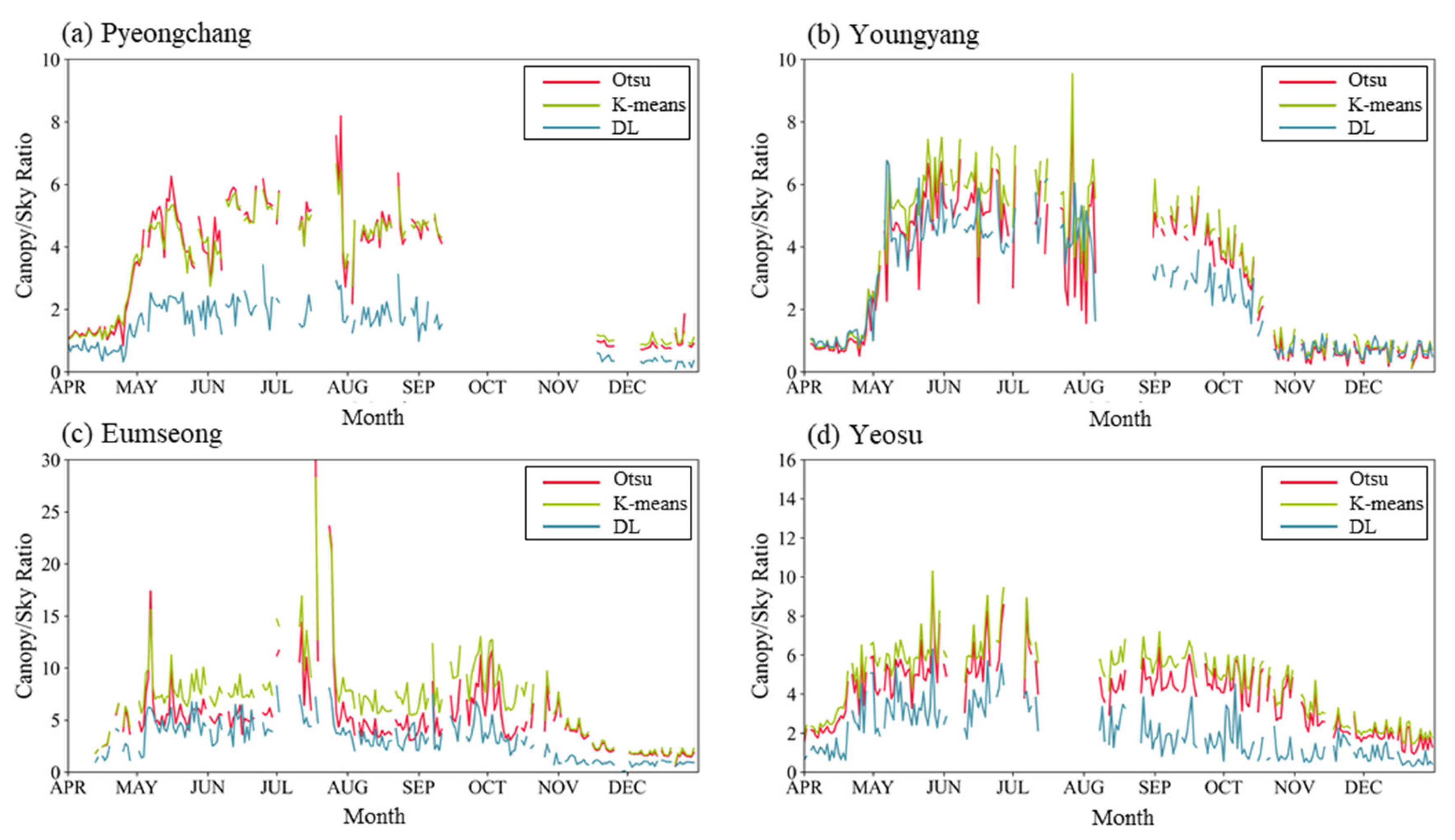
Three binary classification methods—Otsu thresholding (Otsu), K-means clustering (K-means), and deep learning (DL)—were compared for distinguishing between canopy and sky pixels in DHP imagery. The DHP imagery acquired within one hour after sunrise and before sunset at four sites from April to December were binarized: Pyeongchang, Youngyang Eumseong, and Yeosu. We analyzed the binarized images by computing the canopy-to-sky pixel ratio over time, as shown in Figure 2. All four sites showed a similar seasonal pattern, with an increase in the canopy-to-sky ratio from April to May and decreased from October to December. Among the classification methods, K-means (mean 4.3) and Otsu (mean 3.6) classified more pixels as canopy compared to DL (mean 2.1). At Pyeongchang, a DNF site, Otsu (mean 3.2) and K-means (mean 3.2) produced similar mean canopy-to-sky ratios. The variability (standard deviation, SD) of canopy-to-sky ratios was higher for Otsu (mean SD ± 2.5) and K-means (mean SD ± 2.6) compared to DL (mean SD ± 1.5), with all methods showing a marked increase in variability around July and August.

Figure 2. The canopy-to-sky ratio among different binary classification methods—Otsu thresholding (Otsu), K-means clustering (K-means), and deep learning (DL). (a) Pyeongchang, (b) Youngyang, (c) Eumseong, and (d) Yeosu.

Figure 3 shows the Jaccard similarity among three binary classification methods. The similarity was calculated as the number of pixels classified into a common class in two binary images divided by the total number of pixels in the image. A similarity closer to 1 indicates stronger agreement between the two methods. The highest Jaccard similarity was observed between Otsu and K-means (mean 0.88 ± 0.08) across all sites, while lower values were found between DL and Otsu (mean 0.53 ± 0.09) and between DL and K-means (mean 0.51 ± 0.09). Notably, the Eumseong site exhibited seasonal patterns in Jaccard similarity with the largest variation between classification methods: Otsu vs. K-means (mean 0.81 ± 0.12), K-means vs. DL (mean 0.44 ± 0.10), and Otsu vs. DL (mean 0.46 ± 0.09). This deviation was partly explained by the positive correlation between the canopy-to-sky ratio of Otsu and the Jaccard similarity between Otsu and K-means (R² = 0.32), indicating that denser canopy conditions contributed to more consistent classification results between these two methods.

Figure 3. The Jaccard similarity among three binary classification methods: Otsu, K-means, and DL. (a) Pyeongchang, (b) Youngyang, (c) Eumseong, and (d) Yeosu.

3.2. Sensitivity of LAI Estimates to Image Timing in Automated Observations

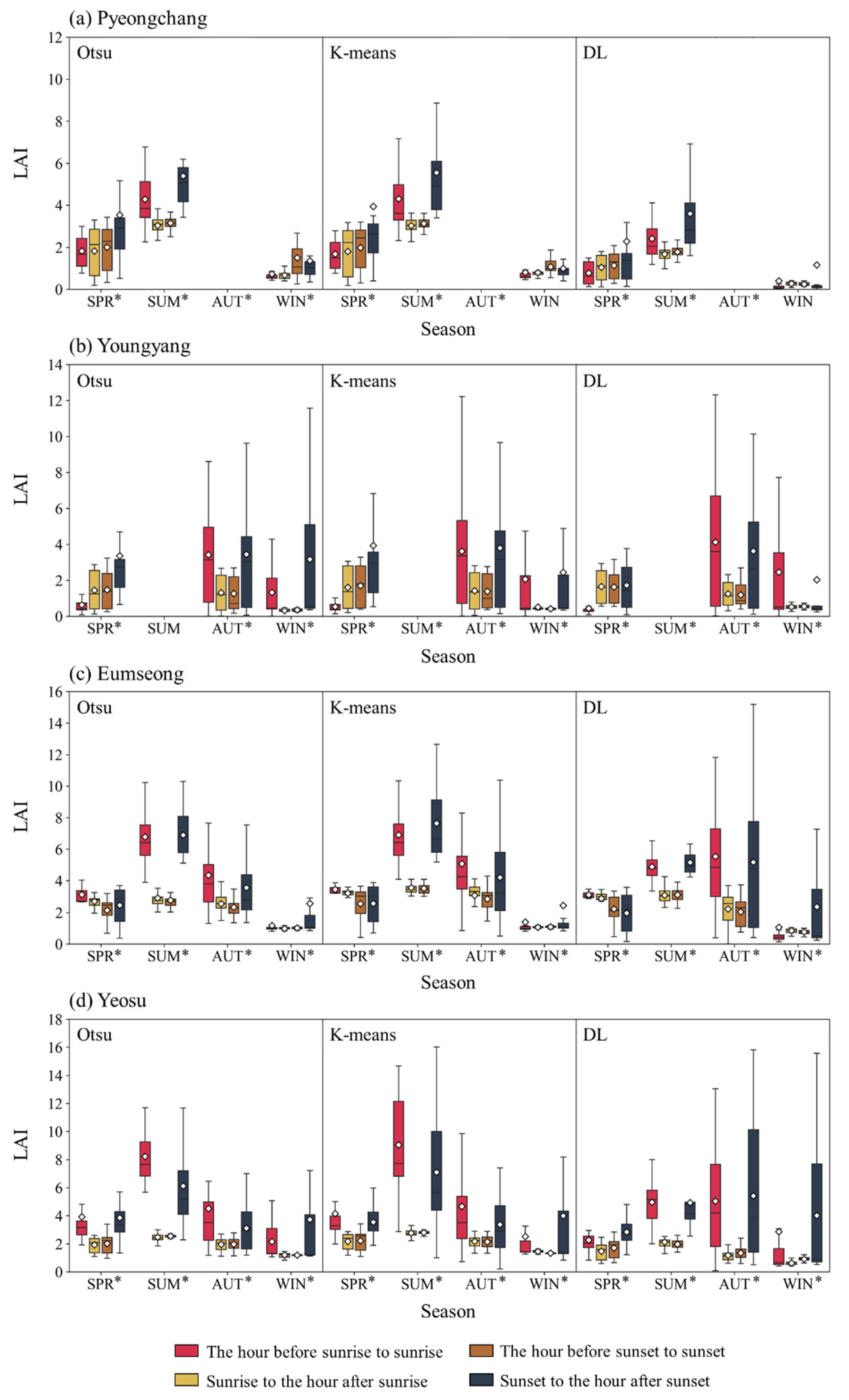
The automatic in situ LAI observation system operates on a fixed timer, limiting data acquisition under optimal conditions. Direct sunlight entering the canopy can cause overexposure at canopy edges, resulting in the underestimation of LAI. Accordingly, it is necessary to quantify how illumination variability from different acquisition timings affects LAI estimates. Figure 4 presents seasonal LAI values estimated from DHP imagery taken in the hour before and after sunrise and sunset. All four sites showed clear phenological patterns, with seasonal average LAI values ranging between 1.43 and 3.86. However, LAI estimates varied depending on the time of image acquisition. The mean SD of LAI in the hour after sunrise was 0.34, compared to 6.33 in the hour before sunrise. A similar trend was observed at sunset, with the mean SD increasing from 0.41 in the hour before sunset to 9.59 in the hour after sunset. This effect was more pronounced during summer and autumn, with differences in mean LAI values ranging from 0.89 to 3.15, depending on the image acquisition time. Among the classification methods, the DL exhibited similar or lower variability in LAI estimates compared to the Otsu and K-means under varying acquisition times. Such results highlight that changes in illumination near sunrise and sunset significantly affected on the variability of LAI estimates (p-value < 0.05).

Figure 4. Seasonal boxplots of leaf area index (LAI) estimated from different image acquisition times across four sites: (a) Pyeongchang, (b) Youngyang, (c) Eumseong, and (d) Yeosu. Statistical significance is indicated by an asterisk next to the x-axis labels when the p-value is less than 0.05. Missing data points indicate locations where data could not be acquired due to power supply issues.

Additionally, LAI derived from gap fraction analysis is determined by two parameters: the effective LAI and the clumping index. As shown in Supplementary Figure S1, the mean clumping index exceeded 0.85 at all sites except for Yeosu in summer (0.80), indicating that seasonal variations in canopy structure have a relatively minor effect on LAI variability. Consequently, it can be suggested that the binary classification results have the greatest influence on LAI estimation.

3.3. Evaluation of Temporal Filtering Methods Using Expert-Interpreted LAI Ranges

Temporal fluctuations in LAI estimates—mainly driven by relative sun-sensor angle and weather variability—were addressed through temporal filtering, as summarized in Table 2. We evaluated the LAI time series using site-specific ranges obtained through manual interpretation. (see Section 2.5). In manual interpretation, the maximum LAI values across 33 sites ranged from 2.46 to 7.95 (mean SD ± 0.61), while the minimum values ranged from 0 to 2.77 (mean SD ± 0.27). In contrast, LAI values obtained from ref. [26] without filtering ranged from 0 to 17.73 across 33 sites. Specifically, the ranges of non-filtered LAI values were 0 to 8.65 at Pyeongchang, 0.01 to 8.39 at Youngyang, 0.05 to 4.80 at Eumseong, and 0 to 6.28 at Yeosu. In comparison, manual LAI measurements showed narrower ranges: from 0.82 to 7.18 at Pyeongchang, 0.02 to 4.07 at Youngyang, 0.22 to 3.19 at Eumseong, and 0.77 to 3.56 at Yeosu. Although regional differences were observed, the non-filtered LAI values generally exhibited higher maximum values than manual LAI, except at the Andong site (p-value < 0.01). Differences in minimum values were not substantial at DBF sites but were larger at ENF sites and particularly pronounced at EBF sites such as Jeju and Wando.

Different temporal filtering methods (Table 2) were applied to the LAI time series data obtained from the automatic in situ LAI observation system, and the LAI range was evaluated against manual interpretation results (Figure 5). The application of temporal filtering reduced the difference between the maximum LAI values and manual interpretation (Figure 5a). In contrast, for the minimum LAI values, certain filtering methods resulted in larger discrepancies compared to unfiltered data (Figure 5b). The smallest difference in maximum LAI was observed with TF14, which applies a seven-day moving average (under the condition of data coverage exceeding 50%) and excludes rainy days as well as the days immediately before and after rainfall events. The additional exclusion of adjacent days further reduced discrepancies, likely by allowing sufficient time for rainwater to evaporate. For minimum LAI values, the smallest differences were found in TF03 (a three-day moving average with exclusion of rainy days) and TF16 (filtering of values beyond one standard deviation within a seven-day window) (Figure 5b). Conversely, methods such as TF06, TF08, TF10, TF12, and TF14, which apply moving averages under the condition of partial data availability (50% threshold), resulted in larger differences for minimum LAI. This suggests that conditional moving averages, especially when applied to periods with sparse observations, may overly smooth local minima and suppress the representation of true low LAI values. We selected TF14 for the subsequent analyses (Supplementary Figure S2), as it showed the smallest deviation from the manual LAI estimates.

Figure 5. Average difference between manual interpretation and the (a) maximum or (b) minimum LAI values obtained from filtered time series from the automatic LAI network across 33 sites. The x-axis represents different temporal filtering methods, as described in Table 2.

4. Discussion

4.1. Stabilization of Binary Classification

The canopy-to-sky ratio exhibited a clear phenological pattern (Figure 2), reflecting the seasonal dynamics of the four deciduous and mixed forest sites. However, large fluctuations in the canopy-to-sky ratio lead to instability in LAI estimates, which propagate substantial inaccuracies in land surface models [35], carbon flux estimations [36], and phenology predictions [37]. The performance of binary classification is sensitive to changing weather conditions (e.g., precipitation, wind, and fog) and stand structural characteristics (e.g., clumping index). Ref. [38] pointed out that heterogeneous sky conditions, blooming effects (i.e., overexposed vegetation pixels), vegetation surface reflection, and mixed pixels can frequently lead to misclassification. In this study, rainfall accounted for the majority of extreme variations in canopy-to-sky ratio in Figure 2. Even when no rainfall was recorded by the weather station, residual water droplets on the camera dome during image acquisition degraded image quality. Such conditions are not adequately represented by precipitation data alone, and the automated detection of water droplet on the dome remains uncertain and technically challenging.

For stable operation of an automated observation network, LAI estimates should remain consistent even over short time intervals. Therefore, we analyzed anomalous values that appeared during consecutive observations. A comparison of binarization methods revealed that K-means and Otsu were more sensitive to sky conditions than the DL approach. As shown in Figure 2c, images acquired at around 5:30 a.m. on 18 July and the following day, 19 July 2024, exhibited substantial variation in canopy-to-sky ratio—from 30.0 to 10.7 using Otsu, and from 28.2 to 12.7 using K-means. In contrast, the DL method demonstrated a more moderate variation, changing from 7.2 to 4.8. These differences indicate that Otsu and K-means methods are influenced by subtle differences in image contrast, affected not only by sky conditions but also by canopy openness. Under low-contrast or uneven illumination, the performance of Otsu thresholding is limited due to the breakdown of its assumption of a bimodal histogram, hampering the determination of a meaningful global threshold [39]. Similarly, K-means clustering suffers from low inter-class variance and sensitivity to centroid initialization, resulting in inaccurate segmentation when intensity differences between regions are subtle [40]. In contrast, the DL-based method leverages contextual information from surrounding pixels, thereby reducing its susceptibility to illumination variability [41]. Collectively, these findings suggest that the DL-based binarization method may offer more stable performance under varying outdoor lighting conditions. However, the temporally stable deep learning method confirmed in this study may be more effective than the Otus and K-means methods for the LAI network continuously observed outdoors. However, it cannot be indicated that deep learning approaches more accurate LAI values than the Otus and K-means methods. To confirm this, further comparative analysis with other methods and actual LAI data is necessary.

4.2. Uncertainty in LAI Estimation Caused by Limitations in Gap Fraction Analysis from an Automated LAI Network

The automatic in situ LAI observation system inevitably experiences fluctuations in binarization performance over consecutive days due to varying weather and illumination conditions during image acquisition. Quantitative evaluation is needed to understand how fluctuations in binarization results contribute to the uncertainty in LAI estimates. As shown in Figure 4, the variability in LAI values was smaller during the periods of both the hour after sunrise and the hour before sunset compared to other times of the day. This finding is consistent with previous studies that recommend taking images during dawn or dusk, when the solar disk remains below the horizon [42,43,44]. In contrast, images captured during midday hours, under strong direct sunlight, may exhibit erroneous classification of leaf edges as sky, potentially compromising the accuracy of LAI estimation. Further research is also needed on optimal data observation methods and strategies in automatic observation networks using DHP sensors, with regard to the variability of LAI values according to sunrise and sunset.

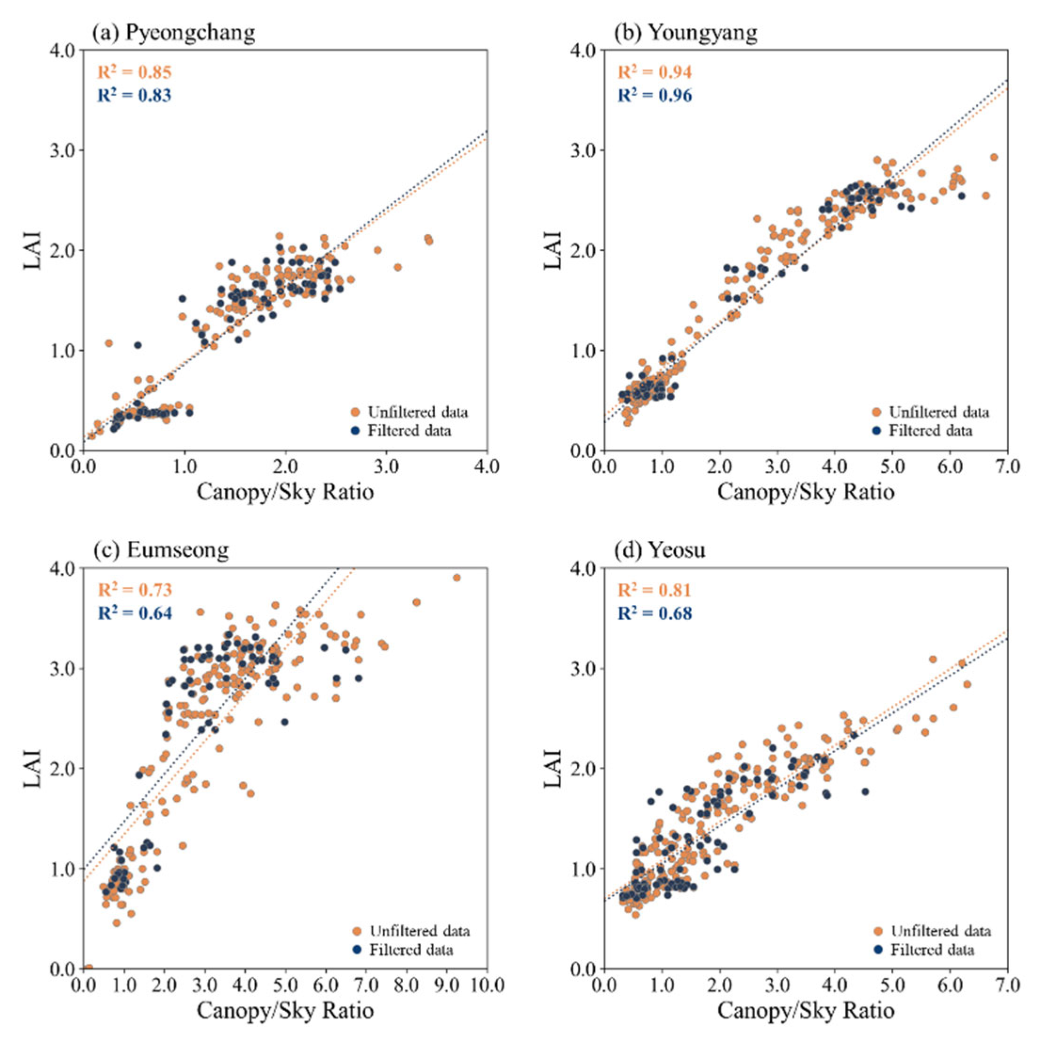
Figure 6 compares the canopy-to-sky ratio and LAI across four different sites—Pyeongchang, Youngyang, Eumseong, and Yeosu—using the DL approach. Both unfiltered and filtered (TF14; see Table 2) data are presented in Figure 6. A positive relationship was observed between LAI and canopy-to-sky ratio across the sites, though the increase in LAI tended to saturate beyond a certain point. The slope of the regression line was highest at the DNF site (Pyeongchang), both before (0.75) and after (0.71) temporal filtering. This was followed by DBF sites (Youngyang and Eumseong) with slopes ranging from 0.46 to 0.51, and the MF site (Yeosu) showing the lowest slopes about 0.38. In Pyeongchang, higher slopes were associated with images where leaf overlap was minimal, and foliage was evenly distributed across the frame (Figure 1a). This indirectly suggests an inverse relationship between LAI and the clumping index. These results suggest greater sensitivity to binarization errors in needleleaf forests, compared to the relatively lower sensitivity observed in broadleaf and mixed forests.

Figure 6. Comparison between canopy-to-sky ratio and LAI at four sites: (a) Pyeongyang, (b) Youngyang, (c) Eumseong, and (d) Yeosu. Orange points represent unfiltered data, and navy points show filtered data using TF14 (see Table 2).

Additionally, the intercept of the regression line in Figure 6 reflects the canopy-to-sky ratio and corresponding LAI values during leaf-off periods, indicative of woody components such as branches and trunks. The intercept varied among sites—Pyeongchang (0.13–0.16), Youngyang (0.24–0.35), Eumseong (0.82–0.88), and Yeosu (0.64–0.70)—indicating that these variations are predominantly influenced by spatial canopy configuration rather than by forest type. Through this analysis, we quantified the uncertainty of LAI estimates and enhanced the understanding of forest structure, particularly regarding woody components.

4.3. Implications of Temporal Filtering for LAI Quality Control

From operational perspective, quality control in the automatic in situ LAI observation system can be implemented through (1) meteorological filtering (e.g., precipitation), (2) image-based quality assessment, and (3) removal of outliers from the LAI time series. Additionally, the diffuse fraction sensor between direct and diffuse radiation can be used to filter images on cloudy or sunny days. Although meteorological filtering (e.g., precipitation-based exclusion) was applied, it alone could not guarantee image quality, which still affected by external factors such as residual water droplets, insect or bird droppings, fallen leaves, and twigs. Given the technical difficulty of quantifying image quality under seasonal changes, removing temporal anomalies from LAI time series was considered the most practical alternative. Specifically, images captured on rainy days, as well as one day before and after each rain event, were excluded. Two different temporal filtering approaches were then applied: (1) moving average smoothing using three-, five-, and seven-day windows, and (2) statistical filtering, which removed values exceeding ±1 standard deviation from the mean within five- or seven-day intervals. These temporal filtering methods effectively removed sudden spikes or anomalies, reducing the absolute difference by 1.5–6.1 for maximum LAI and 0–0.9 for minimum LAI. However, longer moving window periods may introduce unintended smoothing effects, resulting in phase shifts and the misinterpretation of rapid LAI changes (e.g., leaf emergence or senescence) as outliers [45]. Therefore, future studies will explore the use of curve-fitting techniques for more adaptive and robust temporal filtering [46].

The comparison of temporal filtering approaches revealed that deviations from manual LAI values differed between minimum and maximum LAI. For minimum LAI, which typically corresponds to leaf-off periods, deviations generally remained below 1 across all methods. In contrast, maximum LAI exhibited greater variability, with differences exceeding 1.5 depending on the filtering technique. Since maximum LAI is a key variable for capturing the timing and magnitude of vegetation growth in phenology models [47], errors in its estimation can potentially lead to misleading model outcomes. Thus, maximum LAI requires more careful quality control than minimum LAI. On the other hand, in this study, we focused on the maximum and minimum LAI value filtering and did not consider the evaluation and correction of mid-range LAI values. So, for more reliable LAI estimation, further comparative verification using difference methods such as LAI-2200c, harvesting foliage and litter traps were required.

4.4. Actions for Optimizing Automated LAI Network for High-Quality Data Acquisition

Manual observations provide higher precision but are limited in frequency, necessitating trade-offs to optimize automated data quality. One major challenge in automated in situ LAI observation system is capturing images at favorable times of day. Most systems rely on fixed-interval timers, yet environmental variability, equipment vulnerability, and cost-effectiveness make it difficult to implement detailed timing setups in cameras. This study demonstrated that LAI variability was the lowest when images were captured within one hour after sunrise and before sunset. However, seasonal shifts in sunrise and sunset times make it difficult for fixed-time interval timers to consistently capture images under favorable conditions. Increasing image acquisition frequency, combined with an ensemble approach—assuming minimal short-term LAI variability—can reduce illumination-induced binarization errors. In addition, employing context-based deep learning models, such as convolutional neural networks, can improve the robustness of classification under diverse canopy structures and sky conditions.

In addition to illumination conditions, camera configuration also plays a critical role in ensuring consistent image quality and binarization performance. In this study, fisheye cameras were manually configured at each site based on canopy openness and ambient light conditions, and images were stored in JPEG format. Among various parameters, exposure was particularly influential: it often led to underestimation of gap fraction in sparse canopies and overestimation in dense ones. Previous studies suggest that using minimally processed raw images can help mitigate such biases [48], whereas JPEG images tend to be more sensitive to exposure settings and may introduce inconsistencies in gap fraction estimates under dense canopy conditions [49]. As this study used JPEG format, sensitivity to exposure remains a potential source of uncertainty in LAI estimation. So, ref. [21] attempt to reduce the problem of camera exposure settings for LAI observation in the field by using a perforated aluminum screen.

These limitations highlight the need for system-level strategies to enhance the stability and reliability of automated LAI networks. This includes integrating advanced observation techniques, temporal filtering methods, and robust post-processing algorithms to reduce uncertainty. In this context, the present study provides meaningful direction for advancing automated LAI observation systems, particularly in complex forest environments such as those found in South Korea. The National Institute of Forest Science is currently enhancing its in situ LAI observation system with the aim of aligning with the CEOS Land Product Validation framework. Considering the fragmented and heterogeneous nature of Korean forests, this research offers valuable insights into optimizing automated networks for operational use under diverse canopy conditions.

5. Conclusions

The operation of automatic in situ LAI observation networks in mountainous regions is constrained by limited installation locations and the inability to capture measurements at optimal times due to system automation. This study explored practical strategies to enhance system stability and improve the reliability of acquired LAI data.

We evaluated binarization techniques—identified as a major source of variability in DHP-based LAI estimation—under diverse lighting conditions. Deep learning models incorporating contextual information demonstrated greater robustness under uneven illumination compared to conventional methods, such as Otsu and K-means, which rely solely on spectral data. Conducting observations within one hour after sunrise or before sunset was found to be the most effective approach for minimizing variability induced by lighting. Even under favorable illumination, image quality can be compromised by environmental factors such as precipitation or lens contamination (e.g., bird droppings and twigs). Therefore, post-processing using meteorological data and based on LAI time-series patterns is essential to address this. Although outlier removal using moving averages and sliding windows was effective, such methods may misclassify valid data during rapid phenological change, such as leaf emergence or senescence. Future work should focus on developing advanced post-processing techniques and reliability indicators that reflect seasonal dynamics. Despite these limitations, automatic in situ LAI observation systems, providing high temporal resolution and spatial representativeness, are highly valuable for satellite product validation and as inputs to land surface models.

References

- GCOS. The global observing system for climate: Implementation needs. World Meteorol. Organ. 2016, 200, 316. [Google Scholar]
- Law, B.E.; Cescatti, A.; Baldocchi, D.D. Leaf area distribution and radiative transfer in open-canopy forests: Implications for mass and energy exchange. Tree Physiol. 2001, 21, 777–787. [Google Scholar] [CrossRef]
- Rödig, E.; Cuntz, M.; Rammig, A.; Fischer, R.; Taubert, F.; Huth, A. The importance of forest structure for carbon fluxes of the Amazon rainforest. Environ. Res. Lett. 2018, 13, 54013. [Google Scholar] [CrossRef]
- Yan, Y.; Huang, Z.; Yan, K.; Liu, Q. Effects of vertical forest stratification on precipitation material redistribution and ecosystem health of Pinus massoniana in the Three Gorges Reservoir area of China. Sci. Rep. 2024, 14, 27596. [Google Scholar] [CrossRef] [PubMed]
- Xie, X.; Li, A.; Jin, H.; Tan, J.; Wang, C.; Lei, G.; Zhang, Z.; Bian, J.; Nan, X. Assessment of five satellite-derived LAI datasets for GPP estimations through ecosystem models. Sci. Total Environ. 2019, 690, 1120–1130. [Google Scholar] [CrossRef] [PubMed]
- Chase, T.N.; Pielke, R.A.; Kittel, T.G.F.; Nemani, R.; Running, S.W. Sensitivity of a general circulation model to global changes in leaf area index. J. Geophys. Res. Atmos. 1996, 101, 7393–7408. [Google Scholar] [CrossRef]
- Chen, J.M.; Cihlar, J. Plant canopy gap-size analysis theory for improving optical measurements of leaf-area index. Appl. Opt. 1995, 34, 6211–6222. [Google Scholar] [CrossRef]
- Lang, M.; Kuusk, A.; Mõttus, M.; Rautiainen, M.; Nilson, T. Canopy gap fraction estimation from digital hemispherical images using sky radiance models and a linear conversion method. Agric. For. Meteorol. 2010, 150, 20–29. [Google Scholar] [CrossRef]
- White, M.A.; Asner, G.P.; Nemani, R.R.; Privette, J.L.; Running, S.W. Measuring fractional cover and leaf area index in arid ecosystems: Digital camera, radiation transmittance, and laser altimetry methods. Remote Sens. Environ. 2000, 74, 45–57. [Google Scholar] [CrossRef]
- Wang, Y.; Fang, H. Estimation of LAI with the LiDAR technology: A review. Remote Sens. 2020, 12, 3457. [Google Scholar] [CrossRef]
- Baret, F.; Weiss, M.; Allard, D.; Garrigues, S.; Leroy, M.; Jeanjean, H.; Fernandes, R.; Myneni, R.; Privette, J.; Morisette, J.; et al. VALERI: A network of sites and a methodology for the validation of medium spatial resolution land satellite products. Remote Sens. Environ. 2005, 76, 36–39. [Google Scholar]
- Brown, L.A.; Ogutu, B.O.; Dash, J. Tracking forest biophysical properties with automated digital repeat photography: A fisheye perspective using digital hemispherical photography from below the canopy. Agric. For. Meteorol. 2020, 287, 107944. [Google Scholar] [CrossRef]
- Weiss MBaret, F.; Smith, G.J.; Jonckheere, I.; Coppin, P. Review of methods for in situ leaf area index (LAI) determination: Part II. Estimation of LAI, errors and sampling. Agric. For. Meteorol. 2004, 121, 37–53. [Google Scholar] [CrossRef]
- Cohen, W.B.; Justice, C.O. Validating MODIS terrestrial ecology products: Linking in situ and satellite measurements. Remote Sens. Environ. 1999, 70, 1–3. [Google Scholar] [CrossRef]
- Meier, C.; Everhart, J.; Jones, K. TOS Protocol and Procedure: Measurement of Leaf Area Index, K ed.; National Ecological Observatory Network: Boulder, CO, USA, 2018. [Google Scholar]
- Qu, Y.; Han, W.; Fu, L.; Li, C.; Song, J.; Zhou, H.; Bo, Y.; Wang, J. LAINet–A wireless sensor network for coniferous forest leaf area index measurement: Design, algorithm and validation. Comput. Electron. Agric. 2014, 108, 200–208. [Google Scholar] [CrossRef]
- Yang, R.; Liu, L.; Liu, Q.; Li, X.; Yin, L.; Hao, X.; Ma, Y.; Song, Q. Validation of leaf area index measurement system based on wireless sensor network. Sci. Rep. 2022, 12, 4668. [Google Scholar] [CrossRef]
- Chen, Y.; Jiao, S.; Cheng, Y.; Wei, H.; Sun, L.; Sun, Y. LAI-NOS: An automatic network observation system for leaf area index based on hemispherical photography. Agric. For. Meteorol. 2022, 322, 108999. [Google Scholar] [CrossRef]
- Culvenor, D.S.; Newnham, G.J.; Mellor, A.; Sims, N.C.; Haywood, A. Automated in-situ laser scanner for monitoring forest leaf area index. Sensors 2014, 14, 14994–15008. [Google Scholar] [CrossRef]
- Leblanc, S.G.; Chen, J.M. A practical scheme for correcting multiple scattering effects on optical LAI measurements. Agric. For. Meteorol. 2001, 110, 125–139. [Google Scholar] [CrossRef]
- Macfarlane, C.; Ryu, Y.; Ogden, G.N.; Sonnentag, O. Digital canopy photography: Exposed and in the raw. Agric. For. Meteorol. 2014, 197, 244–253. [Google Scholar] [CrossRef]
- Ryu, Y.; Verfaillie, J.; Macfarlane, C.; Kobayashi, H.; Sonnentag, O.; Vargas, R.; Ma, S.; Baldocchi, D.D. Continuous observation of tree leaf area index at ecosystem scale using upward-pointing digital cameras. Remote Sens. Environ. 2012, 126, 116–125. [Google Scholar] [CrossRef]
- Brown, L.A.; Meier, C.; Morris, H.; Pastor-Guzman, J.; Bai, G.; Lerebourg, C.; Gobron, N.; Lanconelli, C.; Clerici, M.; Dash, J. Evaluation of global leaf area index and fraction of absorbed photosynthetically active radiation products over North America using Copernicus Ground Based Observations for Validation data. Remote Sens. Environ. 2020, 247, 111935. [Google Scholar] [CrossRef]
- Brown, L.A.; Morris, H.; Albero, E.; Lopez-Baeza, E.; Tiedemann, F.; Siebicke, L.; Knohl, A.; da Silva Gomes, C.; Bai, G.; Lerebourg, C.; et al. Potential of automated digital hemispherical photography and wireless quantum sensors for routine canopy monitoring and satellite product validation. In Proceedings of the 2021 IEEE International Geoscience and Remote Sensing Symposium IGARSS, Brussels, Belgium, 11–16 July 2021. [Google Scholar]
- Gao, Z.; Chen, Y.; Zhang, Z.; Duan, T.; Chen, J.; Li, A. Continuous Leaf Area Index (LAI) Observation in Forests: Validation, Application, and Improvement of LAI-NOS. Forests 2024, 15, 868. [Google Scholar] [CrossRef]
- Lee, J.; Cha, S.; Lim, J.; Chun, J.; Jang, K. Practical LAI Estimation with DHP Images in Complex Forest Structure with Rugged Terrain. Forests 2023, 14, 2047. [Google Scholar] [CrossRef]
- Bangare, S.L.; Dubal, A.; Bangare, P.S.; Patil, S. Reviewing Otsu’s method for image thresholding. Int. J. Appl. Eng. Res. 2015, 10, 21777–21783. [Google Scholar] [CrossRef]
- Otsu, N. A threshold selection method from gray-level histograms. Automatica 1975, 11, 23–27. [Google Scholar] [CrossRef]
- Xu, X.; Xu, S.; Jin, L.; Song, E. Characteristic analysis of Otsu threshold and its applications. Pattern Recognit. Lett. 2011, 32, 956–961. [Google Scholar] [CrossRef]
- MacQueen, J. Some methods for classification and analysis of multivariate observations. In Proceedings of the Fifth Berkeley Symposium on Mathematical Statistics and Probability, Berkeley, CA, USA, 21 June–18 July 1965 and 27 December 1965–7 January 1966; Volume 1, pp. 281–298. [Google Scholar]
- Dhanachandra, N.; Manglem, K.; Chanu, Y.J. Image segmentation using K-means clustering algorithm and subtractive clustering algorithm. Procedia Comput. Sci. 2015, 54, 764–771. [Google Scholar] [CrossRef]
- Niedballa, J.; Axtner, J.; Döbert, T.F.; Tilker, A.; Nguyen, A.; Wong, S.T.; Fiderer, C.; Heurich, M.; Wilting, A. Imageseg: An R package for deep learning-based image segmentation. Methods Ecol. Evol. 2022, 13, 2363–2371. [Google Scholar] [CrossRef]
- Chianucci, F.; Macek, M. HemispheR: An R Package for Fisheye Canopy Image Analysis. Agric. For. Meteorol. 2023, 336, 109470. [Google Scholar] [CrossRef]
- Origo, N.; Calders, K.; Nightingale, J.; Disney, M. Influence of levelling technique on the retrieval of canopy structural parameters from digital hemispherical photography. Agric. For. Meteorol. 2017, 237, 143–149. [Google Scholar]
- Sabater, J.M.; Rüdiger, C.; Calvet, J.-C.; Fritz, N.; Jarlan, L.; Kerr, Y. Joint assimilation of surface soil moisture and LAI observations into a land surface model. Agric. For. Meteorol. 2008, 148, 1362–1373. [Google Scholar] [CrossRef]
- Liu, Y.; Xiao, J.; Ju, W.; Zhu, G.; Wu, X.; Fan, W.; Li, D.; Zhou, Y. Satellite-derived LAI products exhibit large discrepancies and can lead to substantial uncertainty in simulated carbon and water fluxes. Remote Sens. Environ. 2018, 206, 174–188. [Google Scholar] [CrossRef]
- Lee, L.X.; Whitby, T.G.; Munger, J.W.; Stonebrook, S.J.; Friedl, M.A. Remote sensing of seasonal variation of LAI and fAPAR in a deciduous broadleaf forest. Agric. For. Meteorol. 2023, 333, 109389. [Google Scholar] [CrossRef]
- Glatthorn, J.; Beckschäfer, P. Standardizing the protocol for hemispherical photographs: Accuracy assessment of binarization algorithms. PLoS ONE 2014, 9, e111924. [Google Scholar] [CrossRef]
- Xing, J.; Yang, P.; Qingge, L. Robust 2D Otsu’s algorithm for uneven illumination image segmentation. Comput. Intell. Neurosci. 2020, 2020, 5047976. [Google Scholar] [CrossRef]
- Yang, Z.; Zuo, S.; Zhou, Y.; He, J.; Shi, J. A Review of Document Binarization: Main Techniques, New Challenges, and Trends. Electronics 2024, 13, 1394. [Google Scholar] [CrossRef]
- Baslamisli, A.S.; Groenestege, T.T.; Das, P.; Le, H.-A.; Karaoglu, S.; Gevers, T. Joint learning of intrinsic images and semantic segmentation. In Proceedings of the European Conference on Computer Vision (ECCV), Munich, Germany, 8–14 September 2018; pp. 286–302. [Google Scholar]
- Chen, J.M.; Black, T.A.; Adams, R.S. Evaluation of hemispherical photography for determining plant area index and geometry of a forest stand. Agric. For. Meteorol. 1991, 56, 129–143. [Google Scholar] [CrossRef]
- Leblanc, S.G.; Chen, J.M.; Fernandes, R.; Deering, D.W.; Conley, A. Methodology comparison for canopy structure parameters extraction from digital hemispherical photography in boreal forests. Agric. For. Meteorol. 2005, 129, 187–207. [Google Scholar] [CrossRef]
- Macfarlane, C.; Arndt, S.K.; Livesley, S.J.; Edgar, A.C.; White, D.A.; Adams, M.A.; Eamus, D. Estimation of leaf area index in eucalypt forest with vertical foliage, using cover and fullframe fisheye photography. For. Ecol. Manag. 2007, 242, 756–763. [Google Scholar] [CrossRef]
- Ri, S.; Wang, Q.; Xia, P.; Tsuda, H. Spatiotemporal phase-shifting method for accurate phase analysis of fringe pattern. J. Opt. 2019, 21, 95702. [Google Scholar] [CrossRef]
- Liu, L.; Cao, R.; Chen, J.; Shen, M.; Wang, S.; Zhou, J.; He, B. Detecting crop phenology from vegetation index time-series data by improved shape model fitting in each phenological stage. Remote Sens. Environ. 2022, 277, 113060. [Google Scholar] [CrossRef]
- Zhou, X.; Xin, Q.; Zhang, S.; Delzon, S.; Dai, Y. A prognostic vegetation phenology model to predict seasonal maximum and time series of global leaf area index using climate variables. Agric. For. Meteorol. 2023, 342, 109739. [Google Scholar] [CrossRef]
- Chianucci, F. An overview of in situ digital canopy photography in forestry. Can. J. For. Res. 2020, 50, 227–242. [Google Scholar] [CrossRef]
- Hwang, Y.; Ryu, Y.; Kimm, H.; Jiang, C.; Lang, M.; Macfarlane, C.; Sonnentag, O. Correction for light scattering combined with sub-pixel classification improves estimation of gap fraction from digital cover photography. Agric. For. Meteorol. 2016, 222, 32–44. [Google Scholar] [CrossRef]
Disclaimer/Publisher’s Note: The statements, opinions and data contained in all publications are solely those of the individual author(s) and contributor(s) and not of MDPI and/or the editor(s). MDPI and/or the editor(s) disclaim responsibility for any injury to people or property resulting from any ideas, methods, instructions or products referred to in the content. |
© 2025 by the authors. Licensee MDPI, Basel, Switzerland. This article is an open access article distributed under the terms and conditions of the Creative Commons Attribution (CC BY) license (https://creativecommons.org/licenses/by/4.0/).