

Prediction of Regional Forest Biomass Using Machine Learning: A Case Study of Beijing, China


Abstract
1. Introduction
2. Materials and Methods
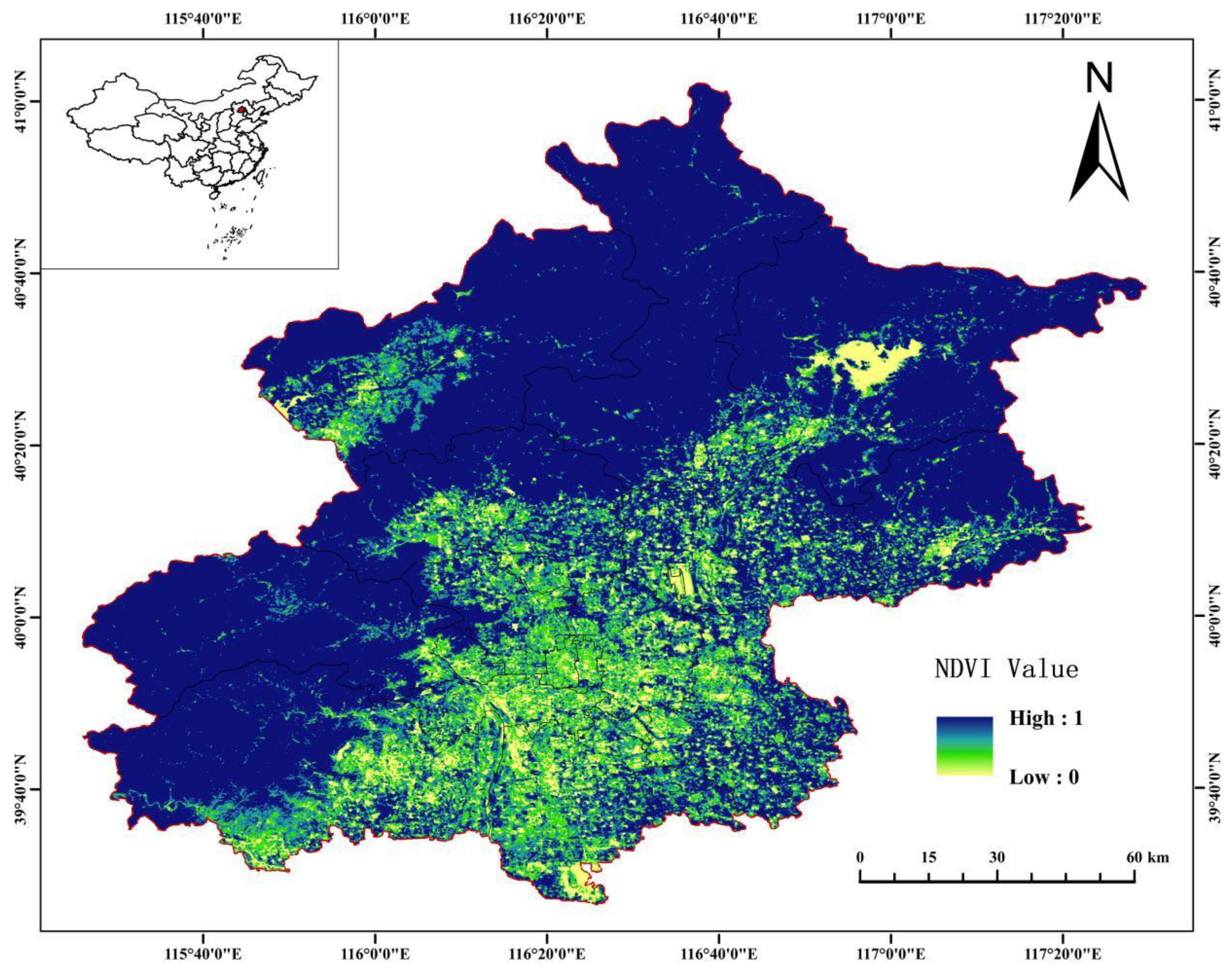
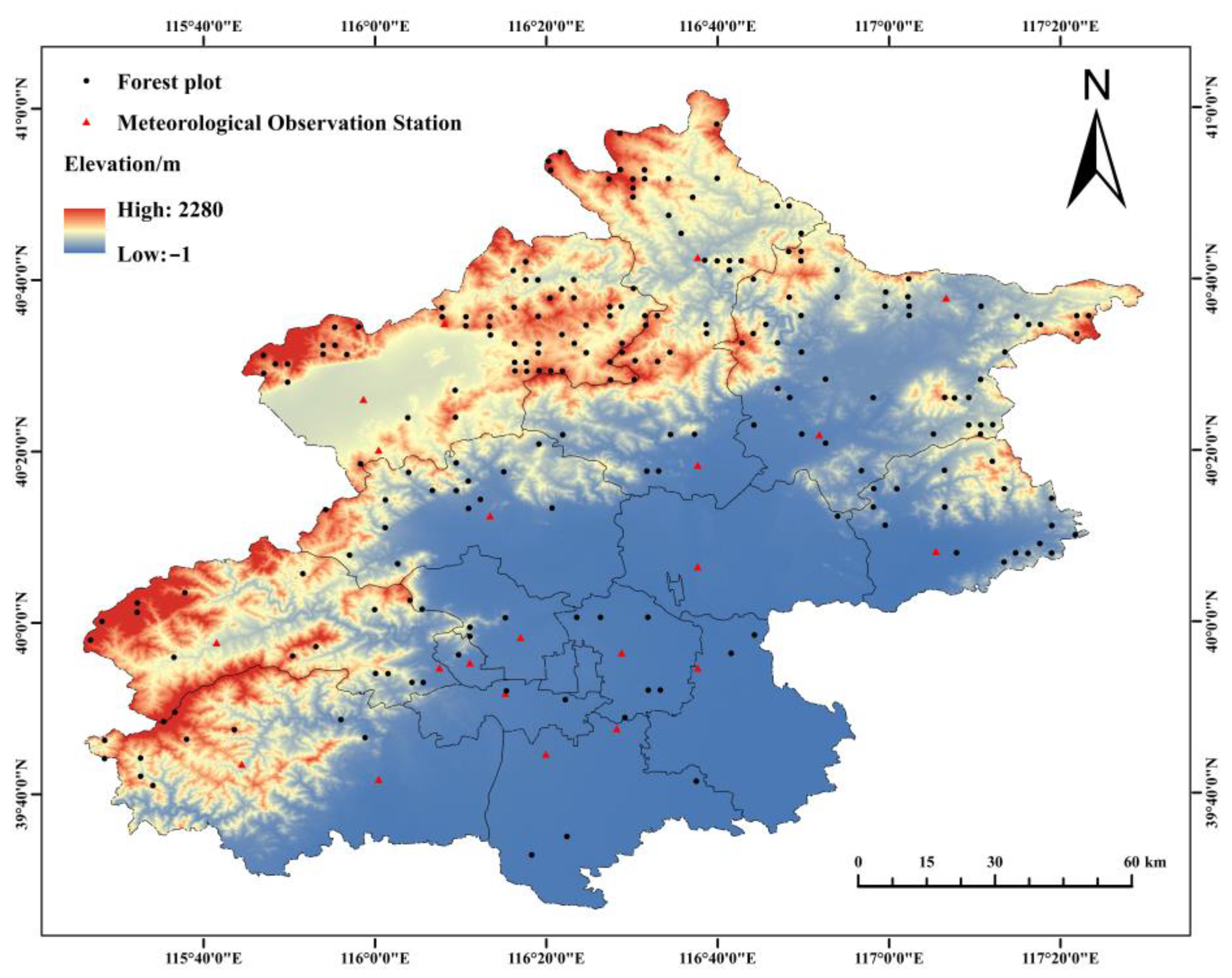
2.1. Overview of the Study Area
2.2. Data Source
2.2.1. National Forest Resource Continuous Inventory Data
2.2.2. Calculating the Basic Biomass of Permanent Plots
2.2.3. Meteorological Data
2.3. Research and Construction Methods
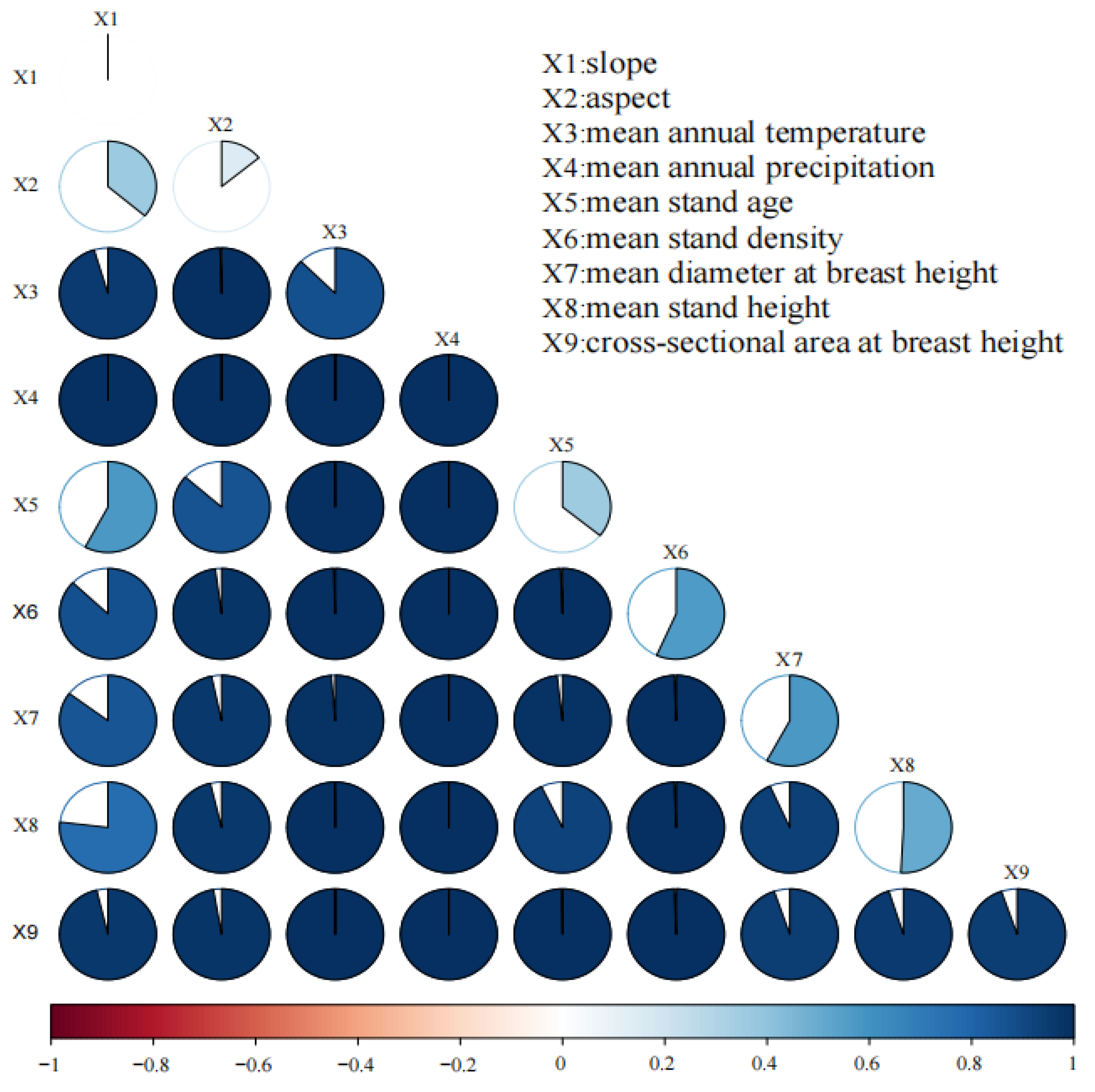
2.3.1. Correlation Analysis
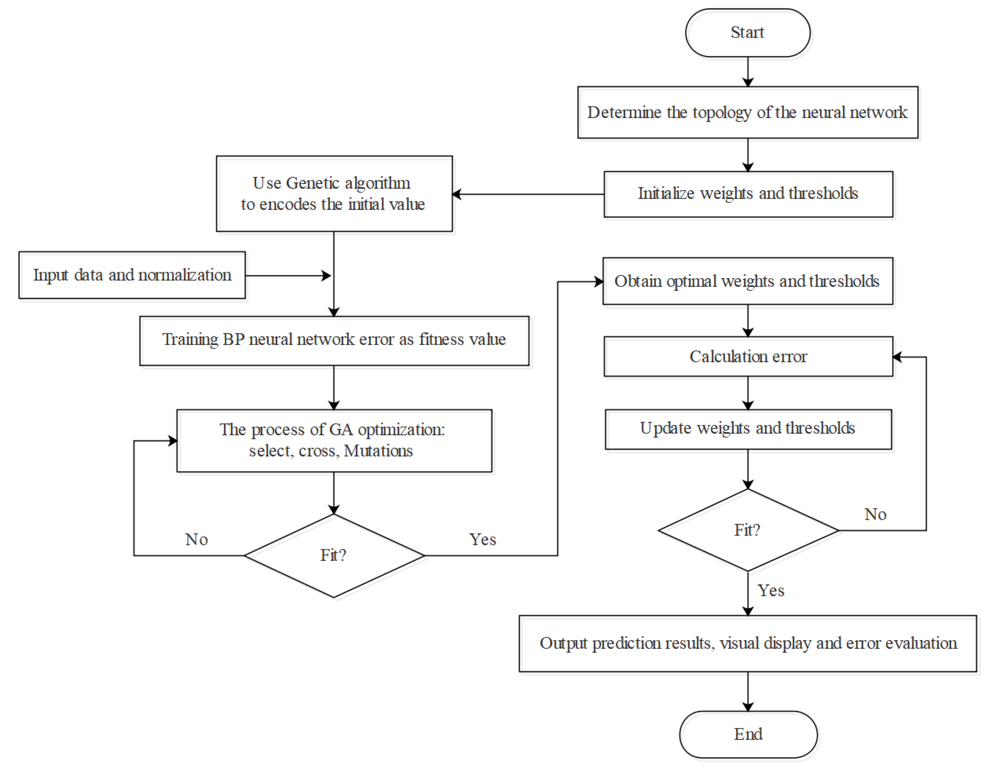
2.3.2. BP-ANN Model
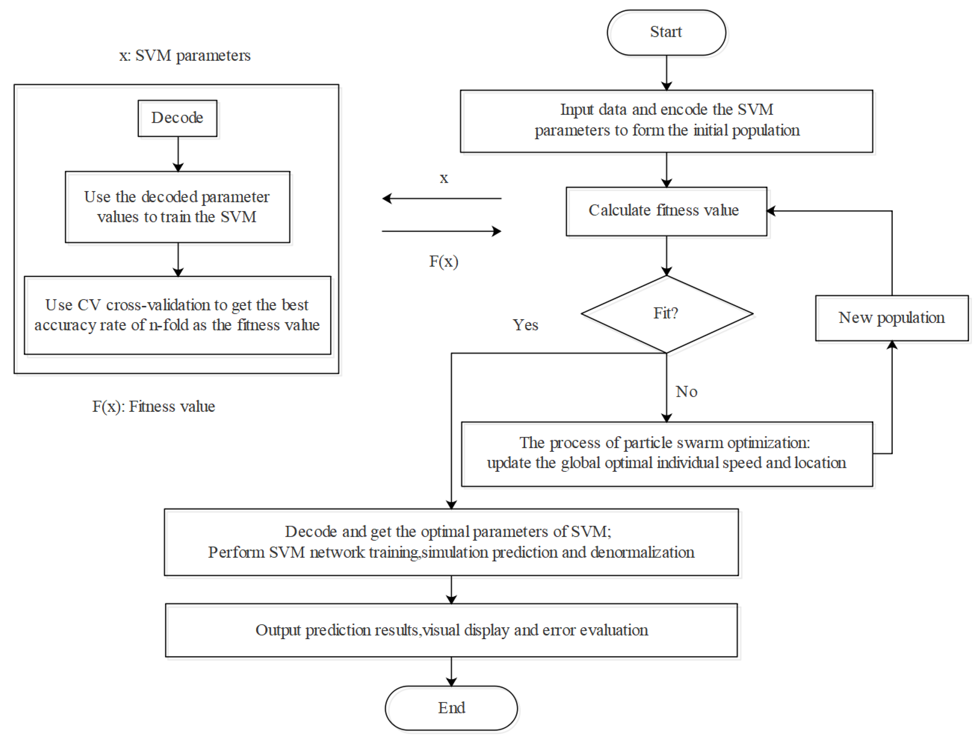
2.3.3. SVM Modeling
2.4. Model Assessment
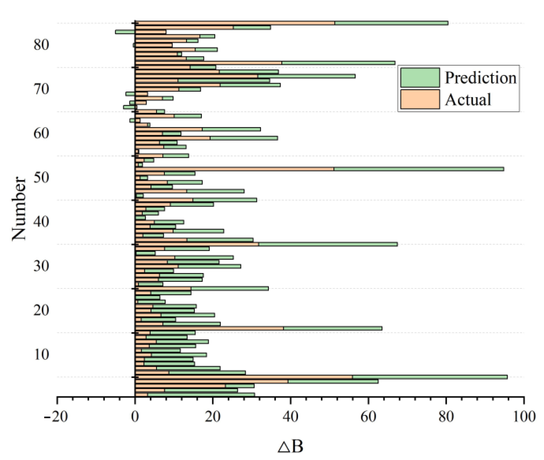
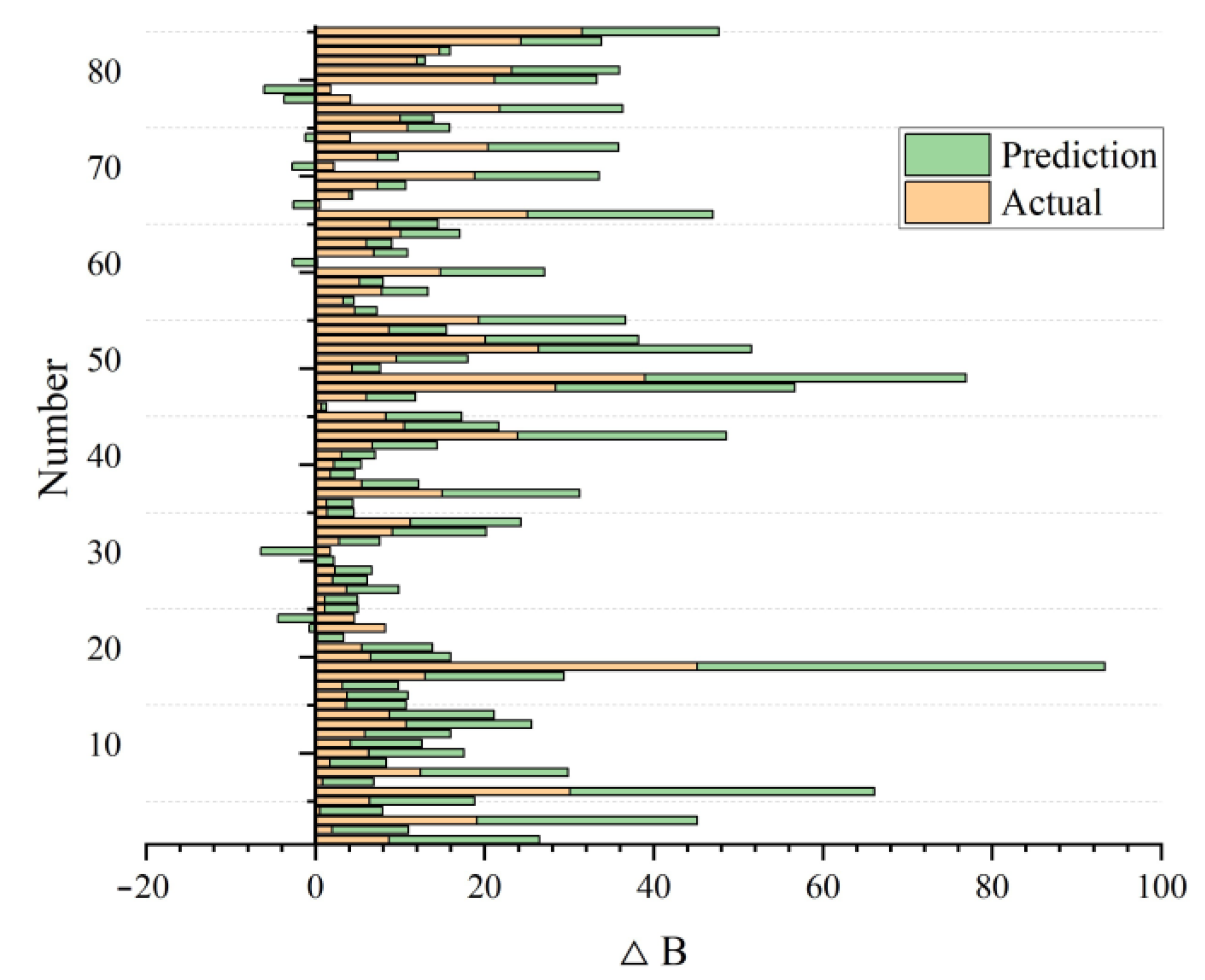
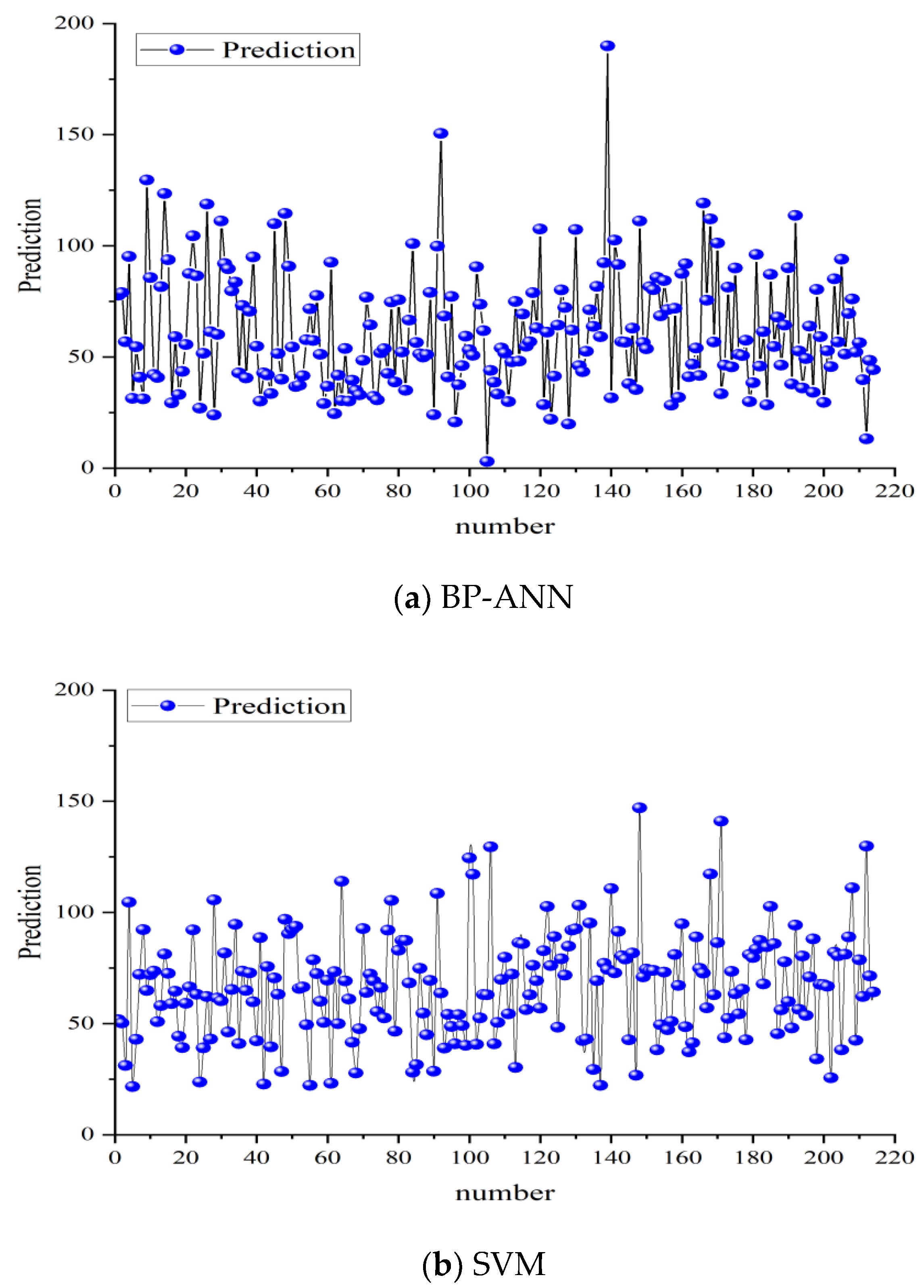
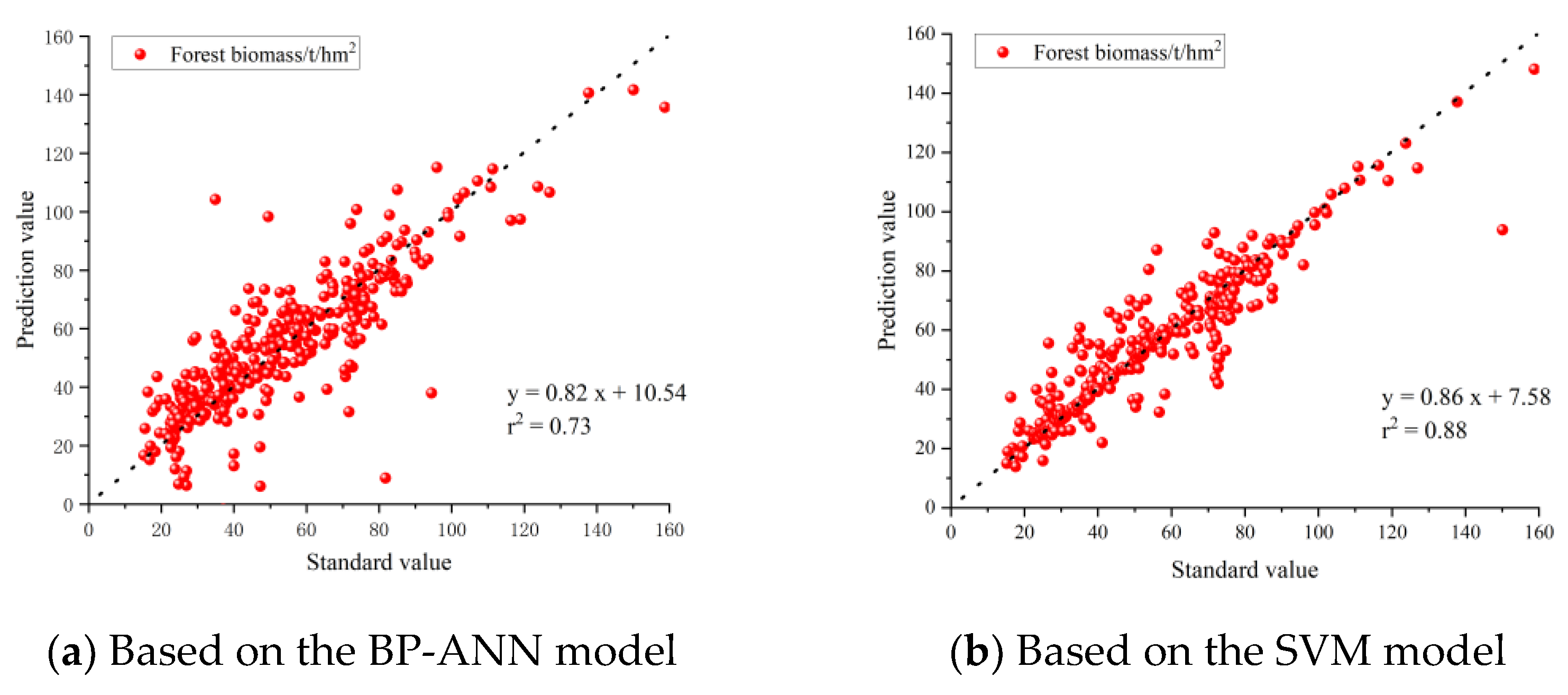
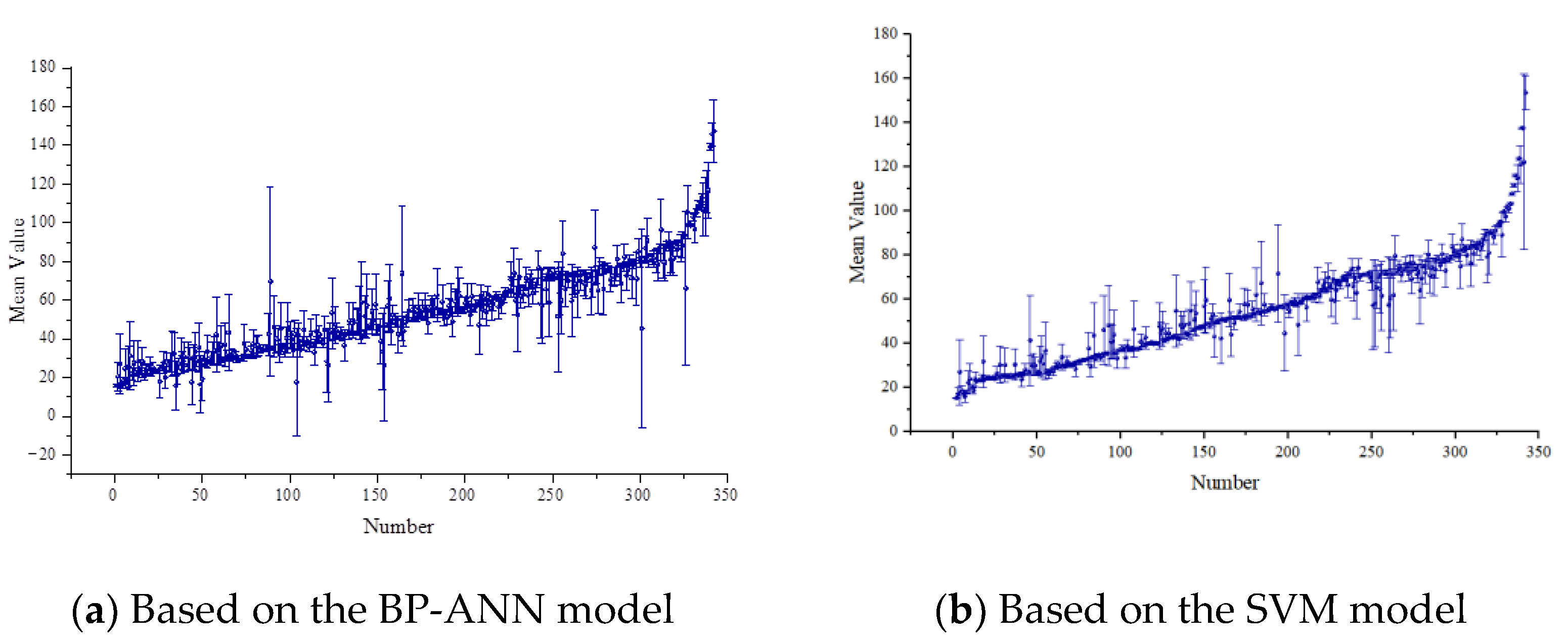
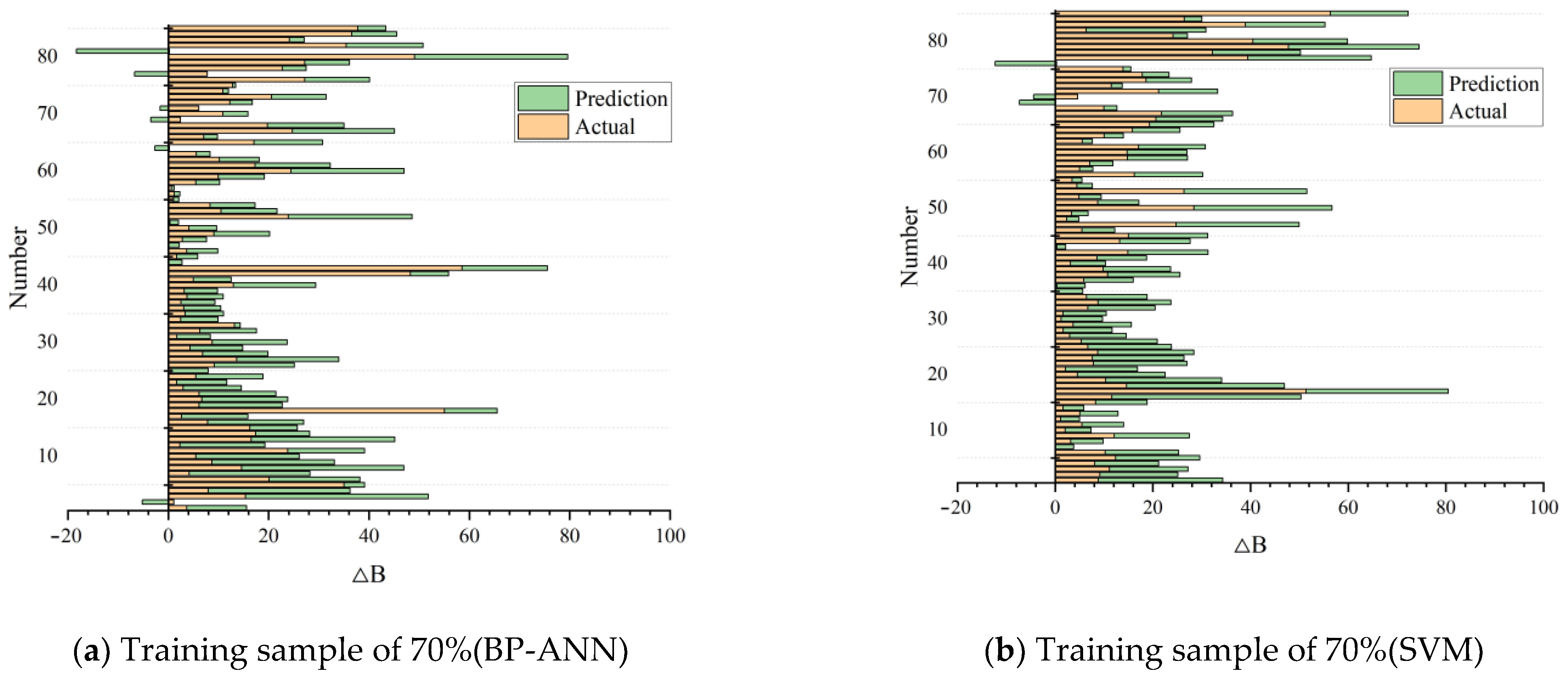
3. Results
4. Discussion
5. Conclusions
Author Contributions
Funding
Data Availability Statement
Acknowledgments
Conflicts of Interest
References
- Singh, A.; Kushwaha, S.K.P.; Nandy, S.; Padalia, H.; Ghosh, S.; Srivastava, A.; Kumari, N. Aboveground Forest Biomass Estimation by the Integration of TLS and ALOS PALSAR Data Using Machine Learning. Remote Sens. 2023, 15, 1143. [Google Scholar] [CrossRef]
- Chi, J.; Zhao, P.; Klosterhalfen, A.; Jocher, G.; Kljun, N.; Nilsson, M.B.; Peichl, M. Forest Floor Fluxes Drive Differences in the Carbon Balance of Contrasting Boreal Forest Stands. Agric. For. Meteorol. 2021, 306, 108454. [Google Scholar] [CrossRef]
- Buchholz, T.; Friedland, A.J.; Hornig, C.E.; Keeton, W.S.; Zanchi, G.; Nunery, J. Mineral Soil Carbon Fluxes in Forests and Implications for Carbon Balance Assessments. GCB Bioenergy 2014, 6, 305–311. [Google Scholar] [CrossRef]
- Primary Productivity of the Biosphere|SpringerLink. Available online: https://link.springer.com/book/10.1007/978-3-642-80913-2 (accessed on 20 March 2023).
- Dai, E.; Wu, Z.; Ge, Q.; Xi, W.; Wang, X. Predicting the Responses of Forest Distribution and Aboveground Biomass to Climate Change under RCP Scenarios in Southern China. Glob. Chang. Biol. 2016, 22, 3642–3661. [Google Scholar] [CrossRef] [PubMed]
- Remote Sensing|Free Full-Text|Estimating the Aboveground Biomass for Planted Forests Based on Stand Age and Environmental Variables. Available online: https://www.mdpi.com/2072-4292/11/19/2270/htm (accessed on 21 March 2023).
- Köhl, M.; Lasco, R.; Cifuentes, M.; Jonsson, Ö.; Korhonen, K.T.; Mundhenk, P.; de Jesus Navar, J.; Stinson, G. Changes in Forest Production, Biomass and Carbon: Results from the 2015 UN FAO Global Forest Resource Assessment. For. Ecol. Manag. 2015, 352, 21–34. [Google Scholar] [CrossRef]
- Zhang, C.; Lu, D.; Chen, X.; Zhang, Y.; Maisupova, B.; Tao, Y. The Spatiotemporal Patterns of Vegetation Coverage and Biomass of the Temperate Deserts in Central Asia and Their Relationships with Climate Controls. Remote Sens. Environ. 2016, 175, 271–281. [Google Scholar] [CrossRef]
- Ribeiro, N.S.; Matos, C.N.; Moura, I.R.; Washington-Allen, R.A.; Ribeiro, A.I. Monitoring Vegetation Dynamics and Carbon Stock Density in Miombo Woodlands. Carbon Balance Manag. 2013, 8, 11. [Google Scholar] [CrossRef]
- Lu, C.; Xu, H.; Zhang, J.; Wang, A.; Wu, H.; Bao, R.; Ou, G. A Method for Estimating Forest Aboveground Biomass at the Plot Scale Combining the Horizontal Distribution Model of Biomass and Sampling Technique. Forests 2022, 13, 1612. [Google Scholar] [CrossRef]
- Ribeiro, N.S.; Saatchi, S.S.; Shugart, H.H.; Washington-Allen, R.A. Washington-Allen, Aboveground biomass and leaf area index(LAI) mapping for Niassa Reserve, northern Mozambique. J. Geophys. Res. 2008, 113, G02S02. [Google Scholar] [CrossRef]
- Saatchi, S.S.; Harris, N.L.; Brown, S.; Lefsky, M.; Mitchard, E.T.; Salas, W.; Zutta, B.R.; Buermann, W.; Lewis, S.L.; Hagen, S.; et al. Benchmark map of forest carbon stocks in tropical regions across three continents. Proc. Natl. Acad. Sci. USA 2011, 108, 9899–9904. [Google Scholar] [CrossRef] [PubMed]
- Magalhães, T.M. Live Above- and Belowground Biomass of a Mozambican Evergreen Forest: A Comparison of Estimates Based on Regression Equations and Biomass Expansion Factors. For. Ecosyst. 2016, 3, 28. [Google Scholar] [CrossRef]
- Guedes, B.S.; Sitoe, A.A.; Olsson, B.A. Allometric Models for Managing Lowland Miombo Woodlands of the Beira Corridor in Mozambique. Glob. Ecol. Conserv. 2018, 13, e00374. [Google Scholar] [CrossRef]
- Lisboa, S.N.; Guedes, B.S.; Ribeiro, N.; Sitoe, A. Biomass Allometric Equation and Expansion Factor for a Mountain Moist Evergreen Forest in Mozambique. Carbon Balance Manag. 2018, 13, 23. [Google Scholar] [CrossRef] [PubMed]
- Ou, Q.; Li, H.; Yang, Y. Factors Affecting the Biomass Conversion and Expansion Factor of Masson Pine in Fujian Province. Acta Ecol. Sin. 2017, 37, 5756–5764. [Google Scholar] [CrossRef]
- Liu, J.; Feng, Z.; Mannan, A.; Khan, T.U.; Cheng, Z. Comparing Non-Destructive Methods to Estimate Volume of Three Tree Taxa in Beijing, China. Forests 2019, 10, 92. [Google Scholar] [CrossRef]
- Fu, L.; Zeng, W.; Tang, S. Individual Tree Biomass Models to Estimate Forest Biomass for Large Spatial Regions Developed Using Four Pine Species in China. For. Sci. 2017, 63, 241–249. [Google Scholar] [CrossRef]
- Claus, A.; George, E. Effect of Stand Age on Fine-Root Biomass and Biomass Distribution in Three European Forest Chronosequences. Can. J. For. Res.-Rev. Can. Rech. For. 2005, 35, 1617–1625. [Google Scholar] [CrossRef]
- Van Den Berge, S.; Vangansbeke, P.; Calders, K.; Vanneste, T.; Baeten, L.; Verbeeck, H.; Krishna Moorthy, S.P.; Verheyen, K. Biomass Expansion Factors for Hedgerow-Grown Trees Derived from Terrestrial LiDAR. BioEnergy Res. 2021, 14, 561–574. [Google Scholar] [CrossRef]
- Li, L.; Zhou, B.; Liu, Y.; Wu, Y.; Tang, J.; Xu, W.; Wang, L.; Ou, G. Reduction in Uncertainty in Forest Aboveground Biomass Estimation Using Sentinel-2 Images: A Case Study of Pinus densata Forests in Shangri-La City, China. Remote Sens. 2023, 15, 559. [Google Scholar] [CrossRef]
- Hopman, H.J.; Chan, S.M.S.; Chu, W.C.W.; Lu, H.; Tse, C.-Y.; Chau, S.W.H.; Lam, L.C.W.; Mak, A.D.P.; Neggers, S.F.W. Personalized Prediction of Transcranial Magnetic Stimulation Clinical Response in Patients with Treatment-Refractory Depression Using Neuroimaging Biomarkers and Machine Learning. J. Affect. Disord. 2021, 290, 261–271. [Google Scholar] [CrossRef]
- Lopez-Serrano, P.M.; Lopez-Sanchez, C.A.; Alvarez-Gonzalez, J.G.; Garcia-Gutierrez, J. A Comparison of Machine Learning Techniques Applied to Landsat-5 TM Spectral Data for Biomass Estimation. Can. J. Remote Sens. 2016, 42, 690–705. [Google Scholar] [CrossRef]
- Pham, T.D.; Yoshino, K.; Le, N.N.; Bui, D.T. Estimating Aboveground Biomass of a Mangrove Plantation on the Northern Coast of Vietnam Using Machine Learning Techniques with an Integration of ALOS-2 PALSAR-2 and Sentinel-2A Data. Int. J. Remote Sens. 2018, 39, 7761–7788. [Google Scholar] [CrossRef]
- Huang, W.; Li, W.; Xu, J.; Ma, X.; Li, C.; Liu, C. Hyperspectral Monitoring Driven by Machine Learning Methods for Grassland Above-Ground Biomass. Remote Sens. 2022, 14, 2086. [Google Scholar] [CrossRef]
- Lopez-Lopez, S.F.; Martinez-Trinidad, T.; Benavides-Meza, H.; Garcia-Nieto, M.; de los Santos-Posadas, H.M. Non-Destructive Method for above-Ground Biomass Estimation of Fraxinus Uhdei (Wenz.) Lingelsh in an Urban Forest. Urban For. Urban Green. 2017, 24, 62–70. [Google Scholar] [CrossRef]
- Urbazaev, M.; Thiel, C.; Cremer, F. Estimation of forest aboveground biomass and uncertainties by integration of field measurements, airborne LiDAR, and SAR and optical satellite data in Mexico. Carbon Balance Manag. 2018, 13, 5. [Google Scholar] [CrossRef]
- Li, Y.; Li, M.; Li, C.; Liu, Z. Forest Aboveground Biomass Estimation Using Landsat 8 and Sentinel-1A Data with Machine Learning Algorithms. Sci. Rep. 2020, 10, 9952. [Google Scholar] [CrossRef]
- Su, H.; Shen, W.; Wang, J.; Ali, A.; Li, M. Machine Learning and Geostatistical Approaches for Estimating Aboveground Biomass in Chinese Subtropical Forests. For. Ecosyst. 2020, 7, 64. [Google Scholar] [CrossRef]
- Smuga-Kogut, M.; Kogut, T.; Markiewicz, R.; Slowik, A. Use of Machine Learning Methods for Predicting Amount of Bioethanol Obtained from Lignocellulosic Biomass with the Use of Ionic Liquids for Pretreatment. Energies 2021, 14, 243. [Google Scholar] [CrossRef]
- HU, Y.; MA, L.; LI, R.; KE, Z.; YANG, J.; LIU, Z. Factor Analysis of Underground Biomass in Forest Ecosystem on the Loess Plateau. Acta Ecol. Sin. 2021, 41, 8643–8653. [Google Scholar] [CrossRef]
- Dulamsuren, C.; Hauck, M.; Bader, M.; Osokhjargal, D.; Oyungerel, S.; Nyambayar, S.; Runge, M.; Leuschner, C. Water Relations and Photosynthetic Performance in Larix Sibirica Growing in the Forest-Steppe Ecotone of Northern Mongolia. Tree Physiol. 2009, 29, 99–110. [Google Scholar] [CrossRef] [PubMed]
- Newton, P.F. Simulating the Potential Effects of a Changing Climate on Black Spruce and Jack Pine Plantation Productivity by Site Quality and Locale through Model Adaptation. Forests 2016, 7, 223. [Google Scholar] [CrossRef]
- Jiang, F.; Sun, H.; Ma, K.; Fu, L.; Tang, J. Improving Aboveground Biomass Estimation of Natural Forests on the Tibetan Plateau Using Spaceborne LiDAR and Machine Learning Algorithms. Ecol. Indic. 2022, 143, 109365. [Google Scholar] [CrossRef]
- Li, X.; Du, H.; Mao, F.; Zhou, G.; Chen, L.; Xing, L.; Fan, W.; Xu, X.; Liu, Y.; Cui, L.; et al. Estimating Bamboo Forest Aboveground Biomass Using EnKF-Assimilated MODIS LAI Spatiotemporal Data and Machine Learning Algorithms. Agric. For. Meteorol. 2018, 256, 445–457. [Google Scholar] [CrossRef]
- Wu, C.; Tao, H.; Zhai, M.; Lin, Y.; Wang, K.; Deng, J.; Shen, A.; Gan, M.; Li, J.; Yang, H. Using Nonparametric Modeling Approaches and Remote Sensing Imagery to Estimate Ecological Welfare Forest Biomass. J. For. Res. 2018, 29, 151–161. [Google Scholar] [CrossRef]
- Fararoda, R.; Reddy, R.S.; Rajashekar, G.; Chand, T.R.K.; Jha, C.S.; Dadhwal, V.K. Improving Forest above Ground Biomass Estimates over Indian Forests Using Multi Source Data Sets with Machine Learning Algorithm. Ecol. Inform. 2021, 65, 101392. [Google Scholar] [CrossRef]
- Mas, J.F.; Flores, J.J. The Application of Artificial Neural Networks to the Analysis of Remotely Sensed Data. Remote Sens. 2008, 29, 617–663. [Google Scholar] [CrossRef]
- Szantoi, Z.; Escobedo, F.J.; Abd-Elrahman, A.; Pearlstine, L.; Dewitt, B.; Smith, S. Classifying spatially heterogeneous wetland communities using machine learning algorithms and spectral and textural features. Environ. Monit. Assess. 2015, 187, 262. [Google Scholar] [CrossRef]
- Foody, G.M.; Cutler, M.E.; McMorrow, J.; Pelz, D.; Tangki, M.; Boyd, D.S. Mapping the biomass of Bornean tropical rain forest from remotely sensed data. Glob. Ecol. Biogeogr. 2001, 10, 379. [Google Scholar] [CrossRef]
- Zhang, C.; Denka Durgan, S.; Sirianni, H.; Mishra, D. Quantification of sawgrass marsh aboveground biomass in the coastal Everglades using object-based ensemble analysis and Landsat data. Remote Sens. Environ. 2017, 204, 366–379. [Google Scholar] [CrossRef]
- Xu, X.; Cao, M.; Li, K. Temporal-Spatial Dynamics of Carbon Storage of Forest Vegetation in China. Prog. Geogr. 2007, 26, 1–10. [Google Scholar]
- Wang, H.; Niu, S.; Shao, X.; Zhang, C. Study on biomass estimation methods of understory shrubs and herbs in forest ecosystem. Acta Pratacult. Sin. 2014, 23, 20–29. [Google Scholar]
- Shen, C.; Lei, X.; Liu, H.; Wang, L.; Liang, W. Potential impacts of regional climate change on site productivity of Larix olgensis plantations in northeast China. Iforest–Biogeosciences For. 2015, 8, 642. [Google Scholar] [CrossRef]
- Sharma, R.P.; Breidenbach, J. Modeling Height-Diameter Relationship for Norway spruce, Scots pine, and downy birch using Norwegian national forest inventory data. For. Sci. Technol. 2015, 11, 44–53. [Google Scholar] [CrossRef]
- Wang, Y.; Lemay, V.; Baker, T.G. Modelling and prediction of dominant height and site index of Eucalyptus globulus plantations using a nonlinear mixed-effects model approach. Can. J. For. Res. 2007, 37, 1390–1403. [Google Scholar] [CrossRef]
- Wang, T.; Wang, G.; Innes, J.L.; Seely, B.; Chen, B. ClimateAP: An Application for Dynamic Local Downscaling of Historical and Future Climate Data in Asia Pacific. Front. Agr. Sci. Eng. 2017, 4, 448–458. [Google Scholar] [CrossRef]
- Wang, T.; Hamann, A.; Spittlehouse, D.L.; Murdock, T.Q. Murdock: ClimateWNA—High-Resolution Spatial Climate Data for Western North America. J. Appl. Meteor. Clim. 2012, 51, 16–29. [Google Scholar] [CrossRef]
- Wang, J.-F.; Li, X.-H.; Christakos, G.; Liao, Y.-L.; Zhang, T.; Gu, X.; Zheng, X.-Y. Geographical Detectors-Based Health Risk Assessment and Its Application in the Neural Tube Defects Study of the Heshun Region, China. Int. J. Geogr. Inf. Sci. 2010, 24, 107–127. [Google Scholar] [CrossRef]
- Dai, S.; Zheng, X.; Gao, L.; Xu, C.; Zuo, S.; Chen, Q.; Wei, X.; Ren, Y. Improving Plot-Level Model of Forest Biomass: A Combined Approach Using Machine Learning with Spatial Statistics. Forests 2021, 12, 1663. [Google Scholar] [CrossRef]
- Fang, J.Y.; Chen, A.P.; Peng, C.H.; Zhao, S.Q.; Ci, L. Changes in Forest Biomass Carbon Storage in China between 1949 and 1998. Science 2001, 292, 2320–2322. [Google Scholar] [CrossRef] [PubMed]
- Jagodzinski, A.M.; Dyderski, M.K.; Gesikiewicz, K.; Horodecki, P. Effects of Stand Features on Aboveground Biomass and Biomass Conversion and Expansion Factors Based on a Pinus Sylvestris L. Chronosequence in Western Poland. Eur. J. For. Res. 2019, 138, 673–683. [Google Scholar] [CrossRef]
- Jagodzinski, A.M.; Dyderski, M.K.; Gesikiewicz, K.; Horodecki, P. Tree and Stand Level Estimations of Abies Alba Mill. Aboveground Biomass. Ann. For. Sci. 2019, 76, 56. [Google Scholar] [CrossRef]
- Wang, G.; Guan, D.; Xiao, L.; Peart, M.R. Forest Biomass-Carbon Variation Affected by the Climatic and Topographic Factors in Pearl River Delta, South China. J. Environ. Manag. 2019, 232, 781–788. [Google Scholar] [CrossRef] [PubMed]
- Yang, J.; Ji, X.; Deane, D.C.; Wu, L.; Chen, S. Spatiotemporal Distribution and Driving Factors of Forest Biomass Carbon Storage in China: 1977–2013. Forests 2017, 8, 263. [Google Scholar] [CrossRef]
- Wang, L.; Silván-Cárdenas, J.L.; Sousa, W.P. Neural Network Classification of Mangrove Species from Multi-seasonal Ikonos Imagery. Photogramm. Eng. Remote Sens. 2008, 74, 921–927. [Google Scholar] [CrossRef]
- Cutler, D.R.; Edwards, T.C., Jr.; Beard, K.H.; Cutler, A.; Hess, K.T.; Gibson, J.; Lawler, J.J. Random Forests for Classification in Ecology. Ecology 2007, 88, 2783–2792. [Google Scholar] [CrossRef] [PubMed]
- Muukkonen, P.; Heiskanen, J. Estimating Biomass for Boreal Forests Using ASTER Satellite Data Combined with Standwise Forest Inventory Data. Remote Sens. Environ. 2005, 99, 434–447. [Google Scholar] [CrossRef]
- Rumelhart, D.E.; Hinton, G.E.; Williams, R.J. Learning representations by back-propagating errors. Nature 1986, 323, 533–536. [Google Scholar] [CrossRef]
- Funahashi, K.-I. On the Approximate Realization of Continuous Mappings by Neural Networks. Neural Netw. 1989, 2, 183–192. [Google Scholar] [CrossRef]
- Chang, C.-C.; Lin, C.-J. LIBSVM: A Library for Support Vector Machines. ACM Trans. Intell. Syst. Technol. 2011, 2, 27. [Google Scholar] [CrossRef]
- Huang, H.; Wang, Y.; Zong, H. Support Vector Machine Classification over Encrypted Data. Appl. Intell. 2022, 52, 5938–5948. [Google Scholar] [CrossRef]
- Dhanda, P.; Nandy, S.; Kushwaha, S.P.S.; Ghosh, S.; Murthy, Y.V.N.K.; Dadhwal, V.K. Optimizing Spaceborne LiDAR and Very High Resolution Optical Sensor Parameters for Biomass Estimation at ICESat/GLAS Footprint Level Using Regression Algorithms. Prog. Phys. Geogr. 2017, 41, 247–267. [Google Scholar] [CrossRef]
- Kim, K.I.; Jung, K.; Park, S.H.; Kim, H.J. Support Vector Machines for Texture Classification. IEEE Trans. Pattern Anal. Mach. Intell. 2002, 24, 1542–1550. [Google Scholar] [CrossRef]
- Zeng, W.; Duo, H.; Lei, X.; Chen, X.; Wang, X.; Pu, Y.; Zou, W. Individual Tree Biomass Equations and Growth Models Sensitive to Climate Variables for Larix Spp. in China. Eur. J. For. Res. 2017, 136, 233–249. [Google Scholar] [CrossRef]
- Zhu, Y.; Liu, K.; Liu, L.; Wang, S.; Liu, H. Retrieval of Mangrove Aboveground Biomass at the Individual Species Level with WorldView-2 Images. Remote Sens. 2015, 7, 12192–12214. [Google Scholar] [CrossRef]
- Han, M.; Xing, Y.; Li, G.; Huang, J.; Cai, L. Comparison of the accuracy of the maximum canopy height and biomass inversion of the data of different GEDI algorithm groups. J. Cent. South Univ. For. Technol. 2022, 42, 72–82. [Google Scholar] [CrossRef]
- Konopka, B.; Pajtik, J.; Moravcik, M.; Lukac, M. Biomass Partitioning and Growth Efficiency in Four Naturally Regenerated Forest Tree Species. Basic Appl. Ecol. 2010, 11, 234–243. [Google Scholar] [CrossRef]
- Santoro, M.; Beaudoin, A.; Beer, C.; Cartus, O.; Fransson, J.B.S.; Hall, R.J.; Pathe, C.; Schmullius, C.; Schepaschenko, D.; Shvidenko, A.; et al. Forest Growing Stock Volume of the Northern Hemisphere: Spatially Explicit Estimates for 2010 Derived from Envisat ASAR. Remote Sens. Environ. 2015, 168, 316–334. [Google Scholar] [CrossRef]
- Che, J. Optimal Sub-Models Selection Algorithm for Combination Forecasting Model. Neurocomputing 2015, 151, 364–375. [Google Scholar] [CrossRef]
- Wang, T.; Zhou, W.; Xiao, J.; Xie, L. Estimating the grassland aboveground biomass based on remote sensing data and machine learning algorithm. J. Glaciol. Geocryol. 2023, 45, 1–10. [Google Scholar]
- Li, X.; Wu, B.; Su, X.; Chen, Y.; Peng, Y.; Yu, Y.; Fan, X. Study on Estimation Model of Eucalyptus Accumulation in Guangxi Based on Decision Tree Integrated Learning. J. Agric. Sci. Technol. 2020, 22, 81–90. [Google Scholar] [CrossRef]
- Saint-Andre, L.; M’bou, A.T.; Mabiala, A.; Mouvondy, W.; Jourdan, C.; Roupsard, O.; Deleporte, P.; Hamel, O.; Nouvellon, Y. Age-Related Equations for above- and below-Ground Biomass of a Eucalyptus Hybrid in Congo. For. Ecol. Manag. 2005, 205, 199–214. [Google Scholar] [CrossRef]
- Niklas, K.; Tiffney, B. The Quantification of Plant Biodiversity Through Time. Philos. Trans. R. Soc. B-Biol. Sci. 1994, 345, 35–44. [Google Scholar] [CrossRef]
- Tamiminia, H.; Salehi, B.; Mahdianpari, M.; Beier, C.M.; Johnson, L.; Phoenix, D.B. A COMPARISON OF DECISION TREE-BASED MODELS FOR FOREST ABOVE-GROUND BIOMASS ESTIMATION USING A COMBINATION OF AIRBORNE LIDAR AND LANDSAT DATA. ISPRS Ann. Photogramm. Remote Sens. Spat. Inf. Sci. 2021, V-3-2021, 235–241. [Google Scholar] [CrossRef]
- Laurance, W.F.; Andrade, A.S.; Magrach, A.; Camargo, J.L.C.; Campbell, M.; Fearnside, P.M.; Edwards, W.; Valsko, J.J.; Lovejoy, T.E.; Laurance, S.G. Apparent Environmental Synergism Drives the Dynamics of Amazonian Forest Fragments. Ecology 2014, 95, 3018–3026. [Google Scholar] [CrossRef]
- Main-Knorn, M.; Cohen, W.B.; Kennedy, R.E.; Grodzki, W.; Pflugmacher, D.; Griffiths, P.; Hostert, P. Monitoring Coniferous Forest Biomass Change Using a Landsat Trajectory-Based Approach. Remote Sens. Environ. 2013, 139, 277–290. [Google Scholar] [CrossRef]
- Oliveira, C.P.d.; Ferreira, R.L.C.; da Silva, J.A.A.; Lima, R.B.d.; Silva, E.A.; Silva, A.F.d.; Lucena, J.D.S.d.; dos Santos, N.A.T.; Lopes, I.J.C.; Pessoa, M.M.d.L.; et al. Modeling and Spatialization of Biomass and Carbon Stock Using LiDAR Metrics in Tropical Dry Forest, Brazil. Forests. 2021, 12, 473. [Google Scholar] [CrossRef]
- Wu, Z.; Dai, E.; Ge, Q.; Xi, W.; Wang, X. Modelling the integrated effects of land use and climate change scenarios on forest aboveground biomass: A case study in Taihe County of China. J. Geogr. Sci. 2017, 27, 205–222. [Google Scholar] [CrossRef]
- Macave, O.A.; Ribeiro, N.S.; Ribeiro, A.I.; Chaúque, A.; Bandeira, R.; Branquinho, C.; Washington-Allen, R. Modelling Aboveground Biomass of Miombo Woodlands in Niassa Special Reserve, Northern Mozambique. Forests 2022, 13, 311. [Google Scholar] [CrossRef]
- Cornejo, S.; Becker, N.; Hemp, A.; Hertel, D. Effects of land-use change and disturbance on the fine root biomass, dynamics, morphology, and related C and N fluxes to the soil of forest ecosystems at different elevations at Mt. Kilimanjaro (Tanzania). Oecologia 2023, 201, 1089–1107. [Google Scholar] [CrossRef]
- Ryan, C.M.; Williams, M.; Grace, J. Above- and Belowground Carbon Stocks in a Miombo Woodland Landscape of Mozambique. Biotropica 2011, 43, 423–432. [Google Scholar] [CrossRef]


| Timepoint | Forest Area (km2) | Forest Coverage (%) | Forest Stock Volume (Million Cubic Meters) |
|---|---|---|---|
| 6 | 5205 | 31.72 | 1038.58 |
| 7 | 5881 | 35.84 | 1425.33 |
| 8 | 7182 | 43.77 | 2437.36 |
| Training Times | Test | Prediction | |||
|---|---|---|---|---|---|
| R2 | MAPE | RMSE | MSE | MAPE | |
| ① | 0.88 | 0.29 | 76.13 | 18.63 | 0.35 |
| ② | 0.86 | 0.31 | 63.57 | 14.88 | 0.48 |
| ③ | 0.91 | 0.25 | 69.46 | 16.02 | 0.33 |
| Model | Test | Prediction | |||
|---|---|---|---|---|---|
| R2 | MAPE | RMSE | MSE | MAPE | |
| ① | 0.91 | 0.23 | 64.25 | 14.15 | 0.43 |
| ② | 0.92 | 0.18 | 60.51 | 8.19 | 0.40 |
| ③ | 0.91 | 0.26 | 61.98 | 13.45 | 0.36 |
| Model | Test | Prediction | |||
|---|---|---|---|---|---|
| R2 | MAPE | RMSE | MSE | MAPE | |
| BP-ANN | 0.67 | 0.51 | 93.34 | 26.52 | 0.86 |
| SVM | 0.74 | 0.36 | 84.07 | 25.86 | 0.60 |
Disclaimer/Publisher’s Note: The statements, opinions and data contained in all publications are solely those of the individual author(s) and contributor(s) and not of MDPI and/or the editor(s). MDPI and/or the editor(s) disclaim responsibility for any injury to people or property resulting from any ideas, methods, instructions or products referred to in the content. |
© 2023 by the authors. Licensee MDPI, Basel, Switzerland. This article is an open access article distributed under the terms and conditions of the Creative Commons Attribution (CC BY) license (https://creativecommons.org/licenses/by/4.0/).
Share and Cite
Liu, J.; Yue, C.; Pei, C.; Li, X.; Zhang, Q. Prediction of Regional Forest Biomass Using Machine Learning: A Case Study of Beijing, China. Forests 2023, 14, 1008. https://doi.org/10.3390/f14051008
Liu J, Yue C, Pei C, Li X, Zhang Q. Prediction of Regional Forest Biomass Using Machine Learning: A Case Study of Beijing, China. Forests. 2023; 14(5):1008. https://doi.org/10.3390/f14051008
Chicago/Turabian StyleLiu, Jincheng, Chengyu Yue, Chenyang Pei, Xuejian Li, and Qingfeng Zhang. 2023. "Prediction of Regional Forest Biomass Using Machine Learning: A Case Study of Beijing, China" Forests 14, no. 5: 1008. https://doi.org/10.3390/f14051008
APA StyleLiu, J., Yue, C., Pei, C., Li, X., & Zhang, Q. (2023). Prediction of Regional Forest Biomass Using Machine Learning: A Case Study of Beijing, China. Forests, 14(5), 1008. https://doi.org/10.3390/f14051008