A Novel Algorithm Based on Geometric Characteristics for Tree Branch Skeleton Extraction from LiDAR Point Cloud

Abstract

More accurate tree models, such as branch skeleton, are needed to acquire forest inventory data. Currently available algorithms for constructing a branch skeleton from a LiDAR point cloud have low accuracy with problems such as irrational connection near trunk bifurcation, excessive central deviation and topological errors. Using the C++ and PCL library, a novel algorithm of the incomplete simulation of tree transmitting water and nutrients (ISTTWN), based on geometric characteristics for tree branch skeleton extraction, was developed in this research. The algorithm is an incomplete simulation of tree transmitting water and nutrients. Improvements were made to improve the time and memory consumption. The result show that the ISTTWN algorithm without any improvements is quite time consuming but has consecutive output. After improvement with iteration, the process is faster and has more detailed output. Breakpoint connection is added to recover continuity. The ISTTWN algorithm with improvements can produce a more accurate skeleton and cost less time than a previous algorithm. The superiority and effectiveness of the method are demonstrated, which provides a reference for the subsequent study of tree modeling and a prospect of application in other fields, such as virtual reality, computer games and movie scenes.

1. Introduction

With the rapid development of LiDAR technology, the highly accurate three-dimensional (3D) point cloud is used to retrieve real-world information in many fields [1]. Currently, the Terrestrial LiDAR Scanner (TLS), Airborne LiDAR Scanner (ALS) and Mobile LiDAR Scanner (MLS) are widely used in forestry applications. The accuracy of TLS can even reach the millimeter level [2] and its collected tree point cloud can help foresters easily acquire forestry parameters, such as DBH, volume, tree height and crown width [3,4]. This can significantly change the nature of forest inventory data collection. The traditional method is time consuming with a high labor cost and relatively low accuracy [5]. Using LiDAR data with better developed algorithms can not only improve efficiency, reduce cost and have better precision, but can also establish 3D tree models which were previously unavailable.

Three-dimensional tree modeling includes branch modeling and leaf modeling. For tree modeling, both are important. However branch modeling is more important for the forest inventory study and there are two main methods: Delaunay triangulation method and the skeleton method. The model obtained by using Delaunay triangulation looks more realistic, but it has difficulty in extracting forest inventory parameters, and the error of morphological parameters is relatively large [6]. In contrast, the skeleton method can overcome these problems. The skeleton refers to a kind of object representation performed by lines characterized by zero thickness and consistent with the connectivity and topology of the original model as the ideal expression [7,8]. The quantitative structure model (QSM) reconstruction algorithm uses the branch skeleton to establish 3D tree model and calculate volume [9].

Shi [10] points out that the extracting algorithms of the branch skeleton from the tree point cloud are mainly divided into three categories—based on voxel space (VS), point clouds contract (PCC) and geometric characteristic (GC). While the GC algorithm is slightly less computationally efficient than PCC, it has reached optimal or equal excellence among three categories in dealing with small offshoots, model topology, overall effect, adjacent offshoots and center deviation. It meets the requirement of relevant studies that sacrifice acceptable time for higher quality modeling. Therefore, skeleton extraction based on GC has always been a popular research topic [11].

Xu et al. [12] developed a general procedure based on GC to produce the branch skeleton: first, the branch point cloud is layered according to certain rules. Each layer contains several branch segments, and they are located in completely different offshoots, and the collection of them is defined as a bins. There are two main layering rules, one which is layering by the similarity of the shortest-path distance from each point to the root point, and the other which is layering by heights. The root point chosen in branch point cloud needs to adequately represent the bottom of the trunk. Then, each bins is clustered into independent branch segments (each segment of a bins is also defined as a bin, however, bins is not simply the plural form of bin) to obtain skeleton nodes. Finally, the skeleton nodes of adjacent layers are connected according to the correct topological relationship.

For this general procedure, the two classification rules and the number of bins are the key factors influencing the model output, as shown in Figure 1, where N represents the number of layers. When using the method of layering by heights, center deviation at the trunk bifurcation is huge, while using the method of layering by the similarity of the shortest-path distance from each point to the root point, the output is relatively better, however, there is still a large deviation near the root. To solve the problem, Wang [13] adopted the method of excavating a partial root to retain accessibility with the certain radius of bin. Each center of bin near the root can be very close to the center of the branch, which implies that the problem can be solved. Generally, the centroid of the bin is used as the center of the bin.

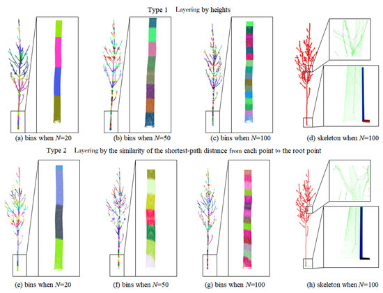
Figure 1. Effects of bins with different layers and the produced skeleton effect under two rules.

Topological correctness is also crucial and is a challenging problem [14]. Model topology using the skeleton can be simply thought of as the connection between the skeleton nodes, that is to say, skeleton lines [15]. Topological correctness means that the skeleton could correctly express the relationship of real offshoots [16]. In other words, skeleton lines that do not accord with the real trunk bifurcation should not be produced. There are two main conditions. One is that there is no error violating the natural law that two or more different parent offshoots cannot produce a same sub offshoot, as shown in Figure 2b. The minimum spanning tree (MST) algorithm (including Prim’s MST algorithm and the Kruskal algorithm) can be used to avoid this problem after the skeleton is produced [17,18]. However, it is difficult to ensure that the sub offshoot in the skeleton this time is connect to its true father offshoot. The other is that there is no error that part of one offshoot is connected with another offshoot, as shown in Figure 2c. Using the described general procedure, there will be incorrectly connected skeleton nodes: although it is easy to ensure skeleton nodes on the same layer cannot be connected with each other, topological errors between different levels can hardly be avoided.

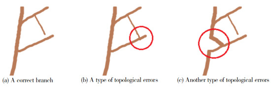
Figure 2. Two types of topological errors.

There has been another classification rule of GC algorithms in recent years—layering by spatial orientation and the radius of branch. This rule is not to layer the point cloud once, but to add extra information at certain places of branch (such as trunk bifurcation), or to keep computing a new reference plane as the cut plane. In essence, this rule still uses information about axial heights and shortest-path distances. Furthermore, because of its complexity, algorithms using this rule are commonly slow. For example, You et al. [19] adopted a simulation of cutting offshoots at trunk bifurcations; TreeQSM [20] used separating offshoots and executing Xu’s general process in every offshoot. Two studies used the B-spline curve and layering relationship to decide the connection of skeleton nodes, respectively. Fan et al. proposed an improvement of TreeQSM named AdQSM [21]. It used a way that combined Delaunay triangulation and graph theory to connect skeleton nodes. Therefore, current GC algorithms are separating the process of producing skeleton nodes and skeleton lines.

Researchers who adopted GC algorithms tried different ways to optimize the output skeleton. Problems such as center deviation can be addressed by three-point average by Li et al. [22]. Interpolation (commonly Hermite method) can be used for making a better connection at trunk bifurcation to make the skeleton appear more beautiful and natural [23]. As for breakpoints, Sun et al. [24] described a method that uses angles calculated with adjacent skeleton lines to determine the topological connection of each breakpoint. In the field of mesh animation, Jacobson et al. [25] listed some skeleton optimization methods with various aspects that have the potential to be used in branch point cloud skeleton extraction.

Runions [26] applied the space colonization algorithm (SCA) to the tree skeleton extraction in 2007 and Shi et al. [27] and Pan [28] tried to improve it. It is difficult to control the type of trunk bifurcations with the SCA, so it is mainly used to simulate the small offshoots using the leaf point cloud when the canopy branch point cloud is incomplete due to occlusion and other reasons [29]. SCA can also be applied to extract the tree skeleton from the ALS point cloud, the branch part of which is not very clear [30].

In the previous discussion, it can be found that there are still some problems in the GC algorithm that deserve to be improved, especially ignoring the internal topological relationship of skeleton nodes. The ecological research shows that trees tend to use the shortest path to transmit water and nutrients for optimizing resource allocation [31]. Based on this natural phenomenon, this research developed a novel algorithm based on GC to extract branch skeleton from the tree point cloud in the way of the incomplete simulation of tree transmitting water and nutrients (ISTTWN). This produced the skeleton nodes and corresponding skeleton lines at same time, which can effectively improve the topological correctness. This ISTTWN algorithm is explained in detail below and was implemented by C++ programming to be verified. Furthermore, different ways have been used to improve the algorithm for reducing the time and memory consumption.

2. Materials

We used a tree point cloud scanned in Chenwei forest farm, Sihong County, Suqian City, Jiangsu Province, China. The tree species corresponding to the point cloud used in this research is American black poplar (Populus deltoides) which was planted in Spring, 2007, and scanned in Autumn, 2019. The tree point clouds were scanned by RIEGL VZ-400i TLS scanner with scanning mode Panorama40, as shown in Table 1. A tree point cloud was randomly selected. Figure 3 is the photo of the sample plot. This tree point cloud will mainly be used for the experiment. In Figure 3, the tree point cloud was already separated into a point cloud of the branch and a point cloud of leaves, which uses a kd-tree with radius $r=0.05$ m.

Table 1. RIEGL VZ-400i scanning mode Panorama40.

Parameters	Values
Scanning resolution	40 mdeg
Scanning time	45 s
Measurement	22.5 Mio
Resolution (20 m)	14 mm
Resolution (50 m)	34 mm
Stations	400

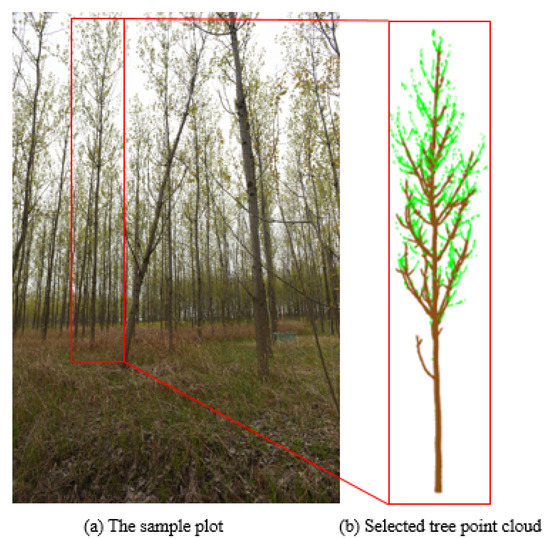
Figure 3. The sample plot and selected tree point cloud.

We also randomly used the tree point clouds of three public tree species provided by Seidel et al. [32] including European beech (Fagus sylvatica L.), European ash (Fraxinus excelsior) and European Oak (Quercus robur L.). Similarly, these clouds have performed the separation of branches and leaves, as shown in Figure 4. Each radius was set as 10x average point cloud intervals. These will mainly be used to verify the universality of the proposed algorithm. The tree ages are beyond 40, beyond 40 and beyond 70.

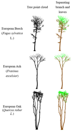
Figure 4. Public tree point clouds.

3. Methods

3.1. Skeleton Production

The general procedure of producing a branch skeleton is to obtain skeleton nodes from the point cloud at each layer, and obtain the topology according to the relationship between layers through certain methods. If the topology is obtained while obtaining skeleton nodes, topological correctness can be notably improved. The “IS” within the ISTTWN algorithm name means “incomplete simulation”. It is necessary to explain the difference between complete and incomplete simulation. Complete simulation directly determines the part used for producing the skeleton node and another part used for continuing the “transmission” based on the step length and the direction of “transmission” without any inputs. The complete simulation is difficult to implement and has poor output, thus, it is not covered here. The incomplete simulation is implemented by using the shortest-path distance from each point to the root point as input, and its execution process is described below and illustrated with Figure 5:

Figure 5. The execution process.

• Divide the unexplored points into appropriate cluster(s) as offshoot(s) and for each offshoot:

  (a)

  Determine the skeleton node according to points within a certain step length.

  (b)

  Use points outside the range as part of the continuing “transmission”.

  (c)

  Remove points within the range from the unexplored points on current offshoot. Use unexplored points at this time as input to repeat Step 1.

3.1.1. Clustering Algorithms Used on Point Cloud

It can be seen from Figure 5c that clustering is needed to classify the unexplored points. However, the number of offshoots at different trunk bifurcations of the same tree is not necessarily the same [33]. Additionally, the computer does not know in advance how many segments should be divided into in situations such as this without any prior information and it is impossible for researchers to tell the computer the quantity of offshoots that every trunk bifurcation has. The best way to deal with this situation is clustering [34]. For point clouds, clustering means that points are segmented in order to group similar structures together when no assumption is made regarding how many segments it should be divided into [35,36,37].

The study used the Point Cloud Library (PCL)—a large scale cross-platform open source C++ programming library for 2D/3D image and point cloud processing [38]. The segment module of PCL provides general clustering algorithms, but not every algorithm is applicable to the branch point cloud. For example, algorithms using normal vectors as the input parameter are not applicable as the uneven surface of many trees could lead to the disorientation of normal vectors even in the same region. For the most common branch point cloud with only 3D spatial information, the study selected the Euclidean cluster extraction (ECE) which is officially provided by PCL and the density-based spatial clustering of applications with noise (DBSCAN), which is not officially provided but currently in mature status.

In principle, ECE uses a K-dimensional tree (kd-tree) to find the neighbors of a point. In the process of label propagation, ECE does not identify noise. After the process, clusters that have less than the allowable minimum number of point(s) in each segment specified in advance will be filtered out. DBSCAN is different when compared with ECE. It propagates the label of each point to its neighbors obtained by neighbor searching with a R*-tree. It detects noise in a way to check whether the number of neighbors of a point reached $MinPts$. The computational complexity of both algorithms is $O(nlogn)$ [39].

Both algorithms require two necessary input parameters—cluster tolerance $Eps$ (or search radius) and an allowable minimum number of point(s) in each segment (cluster) $MinPts$. Among them, Ozkok [40] considered that it is reasonable that $MinPts$ is set to 3 or 4. Sander et al. [41] pointed out that, with $MinPts$ no more than 2, the result will be the same as that of hierarchical clustering with the single link metric, with the dendrogram cut at height $Eps$, but a single-link approach cannot always express the true underlying relationship between clusters, because they only consider just a single pair between two clusters [42]. However, in this research, $MinPts$ needs to be set to 1. On the one hand, after the branches and leaves are separated, all the points in the branch point cloud do not express any information except the branches. Therefore, a cluster with one point is likely to be located on a short sub offshoot connected to a leaf. On the other hand, if $MinPts$ is not equal to 1, it will result in the production of more breakpoints caused by interval segmentation (Detailed in Section 3.2.2) with extremely sparse points which are easily filtered out, causing unnecessary trouble. In this research, DBSCAN produced unreasonable clustering, resulting in the wrong topology, which is described in detail later.

3.1.2. Algorithm Implementation

As is shown in Figure 5, the execution process is based on a base case and is continuous in making progress. In computer data structure, there is also the concept of a tree, and a natural way to define trees is the method of recursion [43]. The idea of recursion can be used for skeleton extraction with the branch point cloud of a real tree as both follow similar rules. The pseudo code of the ISTTWN algorithm is shown in Algorithm 1.

Algorithm 1 ISTTWN algorithm and initializing parameters

Input: Sequence of branch point cloud P, where the ith point $P_i\in P$, $P_1$ must be the root point, and $P_i\ne P_j,\forall i,j=1,2,\cdots ,\mid P\mid ,i\ne j$, $\mid P\mid$ is the size of P; Sequence D that stores the shortest-path distance between each point and the root point, where the ith element $D_i$ represents the shortest-path distance between $P_i$ and the root point $P_1$, if and only if $D_1={\Vert \overrightarrow{P_1{P}_1}\Vert }_2=\mid \mathbf{0}\mid =0$; The longest distance L in sequence D, where $L=max\left(D\right)$; Step length l where $l\ge r,r$ is the search radius that uses the kd-tree previously; Allowable minimum number N of point(s) in each segment when using cluster algorithm; Cluster tolerance t when using cluster algorithm, where $t\ge r$; Output: Set E that stores produced skeleton lines (in the form of ordered pair); 1: $d:=0$                      ▹ Initialize the reached distance 2: $Q:=\mathrm{NULL}$            ▹ Initialize the skeleton point (Not exist Initially) 3: $E:=⌀$                             ▹ Initialize set E 4: function ISTTWN($P,D,L,l,E,N,d,Q,t$) 5:     if $d>L$ or $\mid P\mid =0$ then 6:         return 7:     end if 8:     $S:=\mathrm{Cluster}\_\mathrm{Algorithm}(P,t,N)$       ▹S is the set of segment(s) of P. 9:     foreach segment $S_k\subset S$ do 10:         Initialize $\tilde{D},P^{{}^{\prime }},P^{{}^{″}},D^{{}^{″}}$ 11:         Find out every distance corresponding to $S_k$ from D as $\tilde{D}$, where $\mid \tilde{D}\mid =\mid S_k\mid$ and ${\tilde{D}}_j$ is the distance from the root point $P_1$ to point $S_{k,j}$ 12:         foreach distance ${\tilde{D}}_j\in \tilde{D}$ do 13:            if $d<{\tilde{D}}_j\le d+l$then      ▹ This part is used for getting skeleton point 14:                $P^{{}^{\prime }}\leftarrow P^{{}^{\prime }}\cup \left\{S_{k,j}\right\}$ 15:            else                     ▹ This part is used for recursion 16:                $P^{{}^{″}}\leftarrow P^{{}^{″}}\cup \left\{S_{k,j}\right\}$ 17:                $D^{{}^{″}}\leftarrow D^{{}^{″}}\cup \left\{{\tilde{D}}_j\right\}$ 18:            end if 19:         end for 20:         $Q^{{}^{\prime }}:=\mathrm{Get}\_\mathrm{Centroid}\left(P^{{}^{\prime }}\right)$ 21:         if $Q\ne \mathrm{NULL}$ then 22:            $E\leftarrow E\cup \left\{(Q,Q^{{}^{\prime }})\right\}$ 23:         end if 24:         ISTTWN($P^{{}^{″}},D^{{}^{″}},L,l,E,N,d+l,Q^{{}^{\prime }},t$) 25:     end for 26: end function 27: ISTTWN($P,D,L,l,E,N,d,Q,t$)

From the pseudo code, the algorithm does not involve the root point. As is shown in Figure 5c, the unexplored points are part of the original tree, but can be regarded as two small trees. As is shown in Figure 5d, it is equivalent to continue recursion on two small trees, respectively. Additionally, the algorithm is implemented by recursion, and the recursion depth is $⌈{\displaystyle \frac{L}{l}}⌉$. As recursion is very slow [44], the algorithm needs to be further improved.

3.2. Improvements

3.2.1. Iterative Implementation

In order to improve the speed, the recursive problem is transformed into a non-recursive one. It can be seen in the ISTTWN algorithm that, before recursion, the clustering algorithm is executed to judge the number of clusters that the current branch point cloud has. The recursion depth of the ISTTWN algorithm can be divided into several intervals, each interval is composed of a part of the whole tree. At first, cluster and judge the number of “small trees”, and then make further recursion on each “small tree”, which can effectively reduce the time. Assuming that the interval length is not divisible by step length, the worst situation is that all calculated centroids deviate from centroids calculated by the ISTTWN algorithm, and the probability of this situation is very high. Therefore, in order to ensure that the interval length is divisible by step length, the number h of steps per interval is introduced, where $h\in {\mathbb{N}}^{*}$ and

$$⌈{\displaystyle \frac{L}{h⌈{\displaystyle \frac{L}{l}}⌉}}⌉h⌈{\displaystyle \frac{L}{l}}⌉\ge L.$$

(1)

Formula (1) shows only if the $l\mid L$ and $h\mid L$ equal sign holds; in other cases, the product of the number of interval and interval length must exceed the longest distance. The detailed algorithm is described in Algorithm 2.

Algorithm 2 Iterative ISTTWN algorithm

Input: $P,D,L,l,N,h,t$ Output:E 1: $m:=⌈{\displaystyle \frac{L}{l}}⌉$▹ The number means the result of the longest distance divided by step length 2: $E:=⌀$ 3: for $i:=1\to m$do 4:     $d:=(i-1)l$ 5:     $L^{{}^{\prime }}:=(i+h)l$ 6:     Initialize $P^{{}^{\prime }},D^{{}^{\prime }}$ 7:     for $j:=1\to \mid P\mid$ do 8:         if $d<D_j\le L^{{}^{\prime }}$ then 9:            $P^{{}^{\prime }}\leftarrow P^{{}^{\prime }}\cup \left\{P_j\right\}$ 10:            $D^{{}^{\prime }}\leftarrow D^{{}^{\prime }}\cup \{D_j-d\}$         ▹ Repetition at intervals can be avoided 11:         end if 12:     end for 13:     ISTTWN($P^{{}^{\prime }},D^{{}^{\prime }},L^{{}^{\prime }}-d,l,E,N,0,\mathrm{NULL},t$) 14:     $i\leftarrow i+h$ 15: end for

Another noteworthy thing in the iterative ISTTWN algorithm is that, in order to ensure that the skeleton is connected, the length of each interval needs to include the extra length containing the first segment of the next interval. Take $h=3$ as an example, as shown in Figure 6.

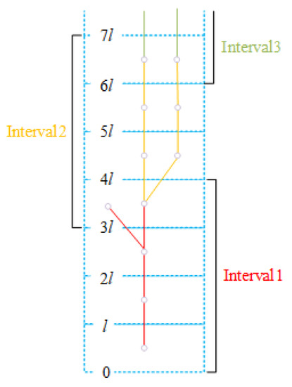
Figure 6. Each interval contains one more step.

3.2.2. Breakpoint Connection

Since the points used in clustering in the ISTTWN algorithm every time are all the unexplored offshoots, and the space of clustering in the iterative ISTTWN algorithm every time is only the points in the interval, the clustering results will have some small differences in not only the skeleton nodes but also in the lines on the steps between intervals, especially in the sheltered canopy. Additionally, although the above $MinPts=1$ can avoid breakpoints with too few clustering points, it will still produce a small amount of breakpoints between the interval segments. These breakpoints always appear in the steps of the interval and interval transition, so they can be handled in the following way:

• Combined with the knowledge of graph theory, because the skeleton lines are stored in ordered pairs, they can be regarded as directed edges, and the indegree and outdegree of each skeleton node can be calculated. The node that is not the root node and whose indegree is 0 must be a breakpoint. Find all breakpoints with this criterion;
• Calculate the distance of the existing longest skeleton lines $d_m$;
• For each breakpoint $P_i$, use a kd-tree to find all neighbor nodes with $r=d_m$. Sequence K consists of these neighbor nodes in the order from near to far, then for each neighbor node $Q_j\in K$:

  (a)

  Skip if $Q_j$ is the node on the offshoot skeleton where $P_i$ is the root node;

  (b)

  Otherwise, the first valid $Q_j$ is the required node. If the outdegree of $Q_j$ is equal to 0, judge further. If the bin of $Q_j$ has some points of bin of $P_i$, they should be the same point and need to be merged. Otherwise, find point R connected to $Q_j$, and replace $R{Q}_j$ with $R{P}_i$; otherwise, add $(Q_j,P_i)$ to the skeleton. End the cycle and start exploring the next breakpoint.

With breakpoint connection, the skeleton is completely connected, and it can then be optimized by skeleton optimization as the branch is not necessarily optimal. Although it seems that the iterative ISTTWN algorithm still needs to deal with breakpoints, it can overcome a defect of the ISTTWN algorithm additionally that if there are two excessively close branches (especially when the circuit is generated), it is easy to be clustered into one segment erroneously. The feasible range to avoid such issue is beyond the set h.

3.2.3. Using Multithreading

Certainly, the iterative ISTTWN algorithm can further split the interval into parallel computing, and multi-threading technology can meet this demand and accelerate the process. It can be expected that each thread shares a relatively average workload as much as possible, and ensures the regularity of the interval in iterative ISTTWN algorithm. In this research, set the maximum number of CPU threads as T, the number of segments that the longest distance can divided into as m and the number of steps per interval as h, and let

$$x=\left(h-⌈{\displaystyle \frac{m}{T}}⌉modh\right)modh+⌈{\displaystyle \frac{m}{T}}⌉.$$

(2)

The allocation of each thread is shown in Table 2.

Table 2. Execution range of each thread of the iterative ISTTWN algorithm using multithreading.

Thread	Starting Distance	End Distance
1	0	$(x+1)l$
2	$xl$	$(2x+1)l$
...	...	...
$i-1(i\le T)$	$(i-1)xl$	$(ix+1)l$
i	$ixl$	$ml$1

¹ During programming, [(i + 1)x + 1]l is used instead of ml to ignore judgement and inequality as [(i + 1)x + 1]l > ml is always true. This is because the iterative ISTTWN algorithm it calls will call the ISTTWN algorithm, and if it encounters void point cloud in recursion, the ISTTWN algorithm will return.

For each thread, each subset of the point cloud and distance sequence ranging from the starting distance to the end distance as parameters $P,D$ executes the iterative ISTTWN algorithm. The goal of this method is only to distribute tasks to different threads without changing tasks that the iterative ISTTWN algorithm determines, so the skeleton produced by this method is the same as the skeleton produced by the iterative ISTTWN algorithm, and similarly, it needs to execute the breakpoint connection.

4. Results

4.1. Applicability of Point Cloud Clustering Algorithm

There are 187,706 points in the branch point cloud of the American black popular. The shortest-path distance from each point in the branch point cloud to the root point is calculated. The longest distance is 26.484700 m. Take the iterative ISTTWN algorithm as an example, as shown in Figure 7 where the input branch point cloud, the skeleton using ECE and the skeleton using DBSCAN are shown. The main parameters are set as $h=10, l=0.05, t=0.05, N=1$.

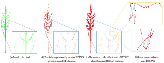
Figure 7. Input branch point cloud and skeletons with different clustering algorithms.

As is shown in Figure 7, the skeleton produced by the iterative ISTTWN algorithm using DBSCAN has serious topological errors, while using ECE does not. Therefore, ECE is used in all later experimental processing.

4.2. Setting of Parameter h

Before discussing, it is worth noting that the point cloud at the root is not processed in this research, and the shortest-path map from each point near the root to the root point presents a radial shape. The size of h determines how much the point cloud covers the original point cloud in each interval after segmentation, but it also affects the speed of time. Increasing the step length l is an effective scheme, but in order to make the skeleton fine enough, it is necessary to adjust h when the step length is small. The smaller the h is set, the faster the speed is. However, due to the small number of points in the subset of the point cloud, it is easy to cause different local clustering results. This is very obvious near the root of the branch point cloud. In the ideal state, the speed is the fastest when $h=1$. However, if h is set too small, unreasonable branches will appear at the root, which will cause trouble for subsequent processing. A convenient way to determine the appropriate value of h is to see whether there are branches at the root of the skeleton established by the point cloud without root pretreatment. For the branch point cloud used in this experiment, the minimum h is set to 5 and as shown in Figure 8, the root skeleton is consistent with the ISTTWN algorithm.

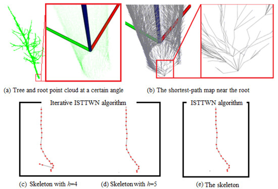
Figure 8. Skeleton near the root.

It has been verified that when the iterative ISTTWN algorithm is combined with breakpoint connection, there is an offshoot that should not appear at the root in the skeleton with $h=4$, and there is only a main branch at $h=5$.

4.3. Algorithm Performance Analysis

One aspect of the algorithm performance analysis is to evaluate the time and space performance of the algorithm. The performance comparison between the proposed algorithm before and after improvement is shown in Table 3.

Table 3. The algorithm efficiency before and after improvement.

Algorithm	Maximum Memory Usage (MB)	Elapsed Time (s)
ISTTWN algorithm	701	313.047
Iterative ISTTWN algorithm with breakpoint connection	5	3.984
Iterative ISTTWN algorithm using multithreading with breakpoint connection	6	1.483

In Table 3, the original algorithm without improvement consumes much more memory and runs very slowly. After transforming the recursive implementation of the original algorithm into an iterative implementation and combining multithreading technology, the time is effectively shortened and the usability is greatly improved.

4.4. Algorithm Universality Verification

Figure 9 shows the branch point clouds and the initial skeletons produced by the ISTTWN algorithm.

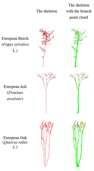
Figure 9. Verification on public tree point clouds.

The detailed parameters of the produced skeletons are shown in Table 4.

Table 4. Detailed parameters of produced skeletons.

Tree Species	Average Point Cloud Intervals (m)	Point Numbers in Branch Point Cloud	Numbers of Skeleton Lines	Elapsed Time (s)
European Beech (Fagus sylvatica L.)	0.016464	163,924	433	6.750
European Ash (Fraxinus excelsior)	0.016659	94,021	931	2.344
European Oak (Quercus robur L.)	0.005627	819,556	3909	27.031

It can be seen from the figure that the skeleton basically conforms to the overall topology of trees, which shows that the algorithm is universal and can handle different tree species. It can be seen from the table that with the increase in the size of the point cloud, the time taken to produce the skeleton generally increases.

5. Discussion

In this section, we will compare the proposed algorithm to Xu et al.’s procedure. The reason we chose Xu et al.’s procedure is that the inner of later improved GC algorithms is always using Xu et al.’s procedure. Furthermore, some extra steps introduced will increase the calculation quantity and reduce the efficiency. If Xu’s algorithm can be improved, the efficiency and effect of other GC algorithms that use Xu’s algorithm as the calling part will naturally be improved. Since most CPUs used in electronic devices now support multithreading technology, it is more realistic to compare the efficiency of the two in multithreading, as shown in Table 5.

Table 5. Comparison between the existing algorithm and the proposed algorithm under multithreading.

Algorithm	Maximum Memory Usage (MB)	Elapsed Time (s)
Xu et al.’s procedure using multithreading with MST	4	2.583
Iterative ISTTWN algorithm using multithreading with breakpoint connection	6	1.483

As shown in Table 5 shows, an iterative ISTTWN algorithm using multithreading with breakpoint connection requires slightly more memory, but is significantly faster than the existing algorithm.

Another aspect that needs to be compared is accuracy. In order to compare which algorithm can better express the real situation of branches, the skeletons and branch point cloud are displayed at the same time, as shown in Figure 10.

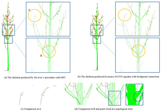
Figure 10. Accuracy comparison of previous and new proposed algorithms.

For easy understanding and description, the skeleton created with Xu et al.’s procedure is called the Xu skeleton and the one created with our method is called the ISTTWN skeleton. As shown in Figure 10c, there are more small offshoots in the ISTTWN skeleton. In other words, the Xu skeleton failed to express some existing offshoots. The Xu skeleton has a bigger center deviation at trunk bifurcation compared with the ISTTWN skeleton. The Xu skeleton showed some incorrect offshoots relationship which is caused by the algorithm itself as the wrong skeleton does not pass through the point cloud. Although the ISTTWN skeleton has similar problems, they can be effectively alleviated by increasing h or l. Apart from in Figure 10d, when such a high-precision skeleton is not required, topological errors such as the sub offshoot connecting to the wrong father offshoots still frequently occur in Xu skeletons, as shown in Figure 11.

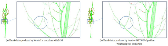
Figure 11. Topological errors in the skeleton produced by Xu et al.’s procedure with MST.

Under this circumstance, the skeleton lines can be convenient for visual statistics. As initial skeletons cannot be used to directly extract parameters, we added the detailed numerical correctness of offshoots. We counted four cases in the skeleton lines: (1) the skeleton line is completely consistent with the point cloud; (2) the trend of the skeleton line is consistent with the branch trend, but not with the point cloud; (3) the skeleton lines are generated where there are no branches (or topological errors occur); and (4) the skeleton lines are produced due to noise. The results are shown in Table 6 and Table 7.

Table 6. Statistics that evaluate the skeleton produced by Xu et al.’s procedure.

Case	(1)	(2)	(3)	(4)
Count	270	45	7	27
Proportion of the whole skeleton lines	77.36%	12.89%	2.01%	7.74%

Table 7. Statistics that evaluate the skeleton produced by the proposed algorithm.

Case	(1)	(2)	(3)	(4)
Count	330	31	0	16
Proportion of the whole skeleton lines	87.53%	8.22%	0%	4.24%

It can be found that, in the case of non-fineness, the algorithm proposed in this study reduces the proportion of errors and some noise effects are eliminated, thus improving the proportion of correctness, and there does not appear to be a Case (3) situation due to topology errors. Therefore, in terms of the numerical aspect, the reliability of the proposed algorithm has been proven.

According to the results, Table 8 shows the summarized comparison of the two algorithms.

Table 8. Comparison of the skeleton extraction algorithms.

Items	Xu et al.’s Procedure with MST	Iterative ISTTWN Algorithm with Breakpoint Connection
Dealing with small offshoots	Worse	Better
Model topology	Many errors (mainly caused by its own defects)	Few errors (mainly caused by point cloud)
Overall effect	Close	Close
Adjacent offshoots	Poor expression	Good expression
Center deviation	Bigger	Smaller
Computational efficiency (using multithreading)	Lower	Higher

Table 8 shows that the ISTTWN skeleton can better express the actual branch connection of the tree. Therefore, it can produce a more accurate skeleton than Xu et al.’s algorithm. Xu et al.’s algorithm was used in QSM, so the ISTTWN algorithm, which has a higher running efficiency and better output skeleton, should be able to be applied to similar applications as well.

6. Conclusions

Based on the results of ecological research, the developed ISTTWN is a representative of a class of algorithms. An implementation of the algorithm is described and several improvements, such as using multithreading and changing from recursion to iterative and connecting breakpoints, were tested. In all, in order to make ISTTWN skeletons have no topological errors, the clustering algorithm should use ECE and the parameters h should be set according to the skeleton near the root. Furthermore, after several improvements, the iterative ISTTWN algorithm using multithreading with breakpoint connection is effective in dealing with the initial skeleton extraction of a branch point cloud. Furthermore, after the random visual verification of public datasets, it is confirmed that the algorithm is universal and can handle different tree branch point clouds. As the skeletons produced by the algorithm are more close to the real topology, such an effect would be helpful for subsequent skeleton optimization.

Through comparison with the existing algorithm, the proposed algorithm is better in comparative items including dealing with small offshoots, model topology, adjacent offshoots, center deviation and computational efficiency. This algorithm improves the accuracy of the skeleton by connecting skeleton points in the process, and greatly improves the efficiency of operation through improvement. In terms of time, the proposed algorithm only needs less than 60% of the time of the existing algorithm. We counted the accuracy of the skeleton in the case of it being not sufficiently fine, and the results showed that the proportion of correct skeleton lines increased by 10%.

Tree modeling is often applied in many other fields such as virtual reality (VR), computer games and movie scenes [45]. For example, motion capture (Mocap) is used to obtain an actor’s characteristic motions [46] to make virtual characters more real, and the method developed in this research can be used in similar fields.

Of course, the proposed algorithm still has some limitations that can be improved.

(1)

The method of using multithreading acceleration proposed in this paper is divided mechanically. Although it can avoid common problems of multithreading, it cannot always make all threads work, so there is still room for improvement.

(2)

The point cloud as input cannot have two offshoots attached. Otherwise, no matter what algorithm, the error shown in Figure 10d cannot be avoided.

(3)

Currently, there are not any reasonable algorithms of the Root Close Algorithm to process the tree point cloud, no modification was made to the original tree point cloud in this research. Thus, when the skeleton is required to be fine enough, the center deviation near the root will inevitably occur. If the root could be processed well in advance or an algorithm of root adjustment can be run after producing the skeleton, a smaller h would be feasible, even $h=1$, as h is just a factor affecting the visual performance of the initial skeleton. In this way, the running speed of the algorithm will be faster and the memory consumption will be less.

(4)

Clustering algorithm is one of the most important factors affecting the accuracy of the tree skeleton. Yang et al. [47] pointed out that the common problems of existing clustering algorithms can be divided into four categories: sensitivity to initial parameters, difficulty in finding optimal clustering, clustering effectiveness and sensitivity to noise data. Each clustering algorithm has more or less of these problems in different application fields. Better clustering algorithms for producing the skeleton of a branch point cloud will be an important research direction. In addition, the integrity of the tree point cloud is also critical. Severe occlusion and large missing data have a huge negative impact on skeleton extraction [48].

References

- He, T.; Liu, Y.; Shen, C.; Wang, X.; Sun, C. Instance-Aware Embedding for Point Cloud Instance Segmentation. In Computer Vision—ECCV 2020; Springer International Publishing: Cham, Switzerland, 2020; pp. 255–270. [Google Scholar] [CrossRef]
- Kunz, M.; Hess, C.; Raumonen, P.; Bienert, A.; Hackenberg, J.; Maas, H.; Härdtle, W.; Fichtner, A.; von Oheimb, G. Comparison of wood volume estimates of young trees from terrestrial laser scan data. iForest-Biogeosci. For. 2017, 10, 451–458. [Google Scholar] [CrossRef]
- Zhang, Y.; Yu, W.; Zhao, X.; Lyu, Y.; Feng, W.; Li, Z.; Hu, S. Interactive tree segmentation and modeling from ALS point clouds. J. Graph. 2021, 42, 599–607. [Google Scholar] [CrossRef]
- Cao, W.; Chen, D.; Shi, Y.; Cao, Z.; Xia, S. Progress and Prospect of LiDAR Point Clouds to 3D Tree Models. Geomat. Inf. Sci. Wuhan Univ. 2021, 46, 203. [Google Scholar] [CrossRef]
- Wang, G.; Li, Q.; Yang, X.; Wang, C. Real Scene Modeling of Forest Based on Airborne LiDAR Data. J. Beijing Univ. Civ. Eng. Archit. 2021, 37, 39–46. [Google Scholar] [CrossRef]
- Gao, S.; Zhang, H.; Liu, M.; Bai, J. Constructing Technology of Tree Branches Delaunay Triangulation. J. Southwest For. Univ. 2013, 33, 62–68. [Google Scholar] [CrossRef]
- Huang, Q. Study on the Method of Constructing Tree Skeleton by Collecting Branches. Master’s Thesis, Hebei Agricultural University, Baoding, China, 2019. [Google Scholar]
- Bournez, E.; Landes, T.; Saudreau, M.; Kastendeuch, P.; Najjar, G. From tls point clouds to 3D models of trees: A comparison OF existing algorithms for 3D tree reconstruction. Int. Arch. Photogramm. Remote. Sens. Spat. Inf. Sci. 2017, XLII-2/W3, 113–120. [Google Scholar] [CrossRef]
- Jin, S.; Zhang, W.; Cai, S.; Shao, J.; Cheng, S.; Xie, D.; Yan, G. Stem and branch volume estimation using terrestrial laser scanning data. Natl. Remote. Sens. Bull. 2021, 3–25. [Google Scholar] [CrossRef]
- Shi, Y. 3D Simulation Theory and Technology of Botanic Tree Based on Scattered Point Cloud; Tongji University Press: Shanghai, China, 2018. [Google Scholar]
- Hu, H.; Li, Z.; Jin, X.; Deng, Z.; Chen, M.; Shen, Y. Curve Skeleton Extraction From 3D Point Clouds Through Hybrid Feature Point Shifting and Clustering. Comput. Graph. Forum 2020, 39, 111–132. [Google Scholar] [CrossRef]
- Xu, H.; Gossett, N.; Chen, B. Knowledge and heuristic-based modeling of laser-scanned trees. ACM Trans. Graph. 2007, 26, 19. [Google Scholar] [CrossRef]
- Wang, B. Studies on Automatic 3D Reconstruction Techniques of Trees Based on Terrestrial LiDAR Point Clouds. Master’s Thesis, University of Electronic Science and Technology of China, Chengdu, China, 2015. [Google Scholar] [CrossRef]
- Liang, P.; Zhou, G.Q.; Lu, Y.L.; Zhou, X.; Song, B. Hole-filling algorithm for airborne lidar point cloud data. Int. Arch. Photogramm. Remote. Sens. Spat. Inf. Sci. 2020, XLII-3/W10, 739–745. [Google Scholar] [CrossRef]
- Song, T.; Liu, W.; Liu, J. Method of linear skeleton topological similarity measurement based on skeleton tree. Infrared Laser Eng. 2005, 34, 74–79. [Google Scholar]
- Lecigne, B.; Delagrange, S.; Taugourdeau, O. Annual Shoot Segmentation and Physiological Age Classification from TLS Data in Trees with Acrotonic Growth. Forests 2021, 12, 391. [Google Scholar] [CrossRef]
- Guo, J. Geometric Modeling of Individual Trees Considering the Distribution of Canopy Leaf Area Index. Master’s Thesis, Fuzhou University, Fuzhou, China, 2017. [Google Scholar]
- Zhang, J.; Kang, B.S.; Jiang, B.; Zhang, D. A novel sketch-based 3D model retrieval approach based on skeleton. Int. J. Inform. Commun. Technol. (IJ-ICT) 2019, 8, 1. [Google Scholar] [CrossRef]
- You. Stem Form Measurement Based on Point Cloud Data. Ph.D. Thesis, Chinese Academy of Forestry, Beijing, China, 2016. [Google Scholar]
- Raumonen, P.; Kaasalainen, M.; Åkerblom, M.; Kaasalainen, S.; Kaartinen, H.; Vastaranta, M.; Holopainen, M.; Disney, M.; Lewis, P. Fast Automatic Precision Tree Models from Terrestrial Laser Scanner Data. Remote Sens. 2013, 5, 491–520. [Google Scholar] [CrossRef]
- Fan, G.; Nan, L.; Dong, Y.; Su, X.; Chen, F. AdQSM: A New Method for Estimating Above-Ground Biomass from TLS Point Clouds. Remote Sens. 2020, 12, 3089. [Google Scholar] [CrossRef]
- Li, R.; Bu, G.; Wang, P. An Automatic Tree Skeleton Extracting Method Based on Point Cloud of Terrestrial Laser Scanner. Int. J. Opt. 2017, 2017, 5408503. [Google Scholar] [CrossRef]
- Jiang, S.; Pan, Z.; Feng, Z.; Guan, Y.; Ren, M.; Ding, Z.; Chen, S.; Gong, H.; Luo, Q.; Li, A. Skeleton optimization of neuronal morphology based on three-dimensional shape restrictions. BMC Bioinform. 2020, 21, 395. [Google Scholar] [CrossRef] [PubMed]
- Sun, J.; Wang, P.; Li, R.; Zhou, M. Fast tree skeleton extraction using voxel thinning based on tree point cloud. Remote Sens. 2021, 14, 2558. [Google Scholar] [CrossRef]
- Jacobson, A.; Deng, Z.; Kavan, L.; Lewis, J. Skinning: Real-time Shape Deformation. In Proceedings of the ACM SIGGRAPH 2014 Courses, Vancouver, BC, Canada, 10–14 August 2014. [Google Scholar]
- Runions, A.; Lane, B.; Prusinkiewicz, P. Modeling Trees with a Space Colonization Algorithm. In Proceedings of the Eurographics Workshop on Natural Phenomena, NPH, Prague, Czech, 10–14 September 2007. [Google Scholar] [CrossRef]
- Shi, Y.; He, P.; Hu, S.; Zhang, Z.; Geng, N.; He, D. Reconstruction Method of Tree Geometric Structures from Point Clouds Based on Angle-constrained Space Colonization Algorithm. Trans. Chin. Soc. Agric. Mach. 2018, 49, 207–216. [Google Scholar] [CrossRef]
- Pan, Z. The Research on Single Broad-leaved Tree Visualization Simulation Based on Three-dimensional Point Cloud. Master’s Thesis, Nanjing Forestry University, Nanjing, China, 2020. [Google Scholar]
- Chaudhury, A.; Godin, C. Skeletonization of Plant Point Cloud Data Using Stochastic Optimization Framework. Front. Plant Sci. 2020, 11, 773. [Google Scholar] [CrossRef]
- Hu, S.; Li, Z.; Zhang, Z.; He, D.; Wimmer, M. Efficient tree modeling from airborne LiDAR point clouds. Comput. Graph. 2017, 67, 1–13. [Google Scholar] [CrossRef]
- Dong, Y.; Fan, G.; Zhou, Z.; Liu, J.; Wang, Y.; Chen, F. Low Cost Automatic Reconstruction of Tree Structure by AdQSM with Terrestrial Close-Range Photogrammetry. Forests 2021, 12, 1020. [Google Scholar] [CrossRef]
- Seidel, D.; Annighöfer, P.; Thielman, A.; Seifert, Q.; Thauer, J.H.; Glatthorn, J.; Ehbrecht, M.; Kneib, T.; Ammer, C. Predicting Tree Species From 3D Laser Scanning Point Clouds Using Deep Learning. Front. Plant Sci. 2021, 12, 635440. [Google Scholar] [CrossRef] [PubMed]
- Zhu, Z. Garden Plant Modeling Technology; China Forestry Publishing House: Beijing, China, 2006. (In Chinese) [Google Scholar]
- Zhou, Z. Machine Learning; Tsinghua University Press: Beijing, China, 2016. [Google Scholar]
- Johnson, R.A.; Wichern, D.W. Applied Multivariate Statistical Analysis, 6th ed.; Pearson: London, UK, 2008. [Google Scholar]
- Guo, H. Point Cloud Library PCL from Introduction to Mastery; China Machine Press: Beijing, China, 2019. (In Chinese) [Google Scholar]
- Rusu, R.B. Semantic 3D Object Maps for Everyday Manipulation in Human Living Environments. Ph.D. Thesis, The Technical University of Munich, München, Germany, 2009. [Google Scholar] [CrossRef]
- Rusu, R.B.; Cousins, S. 3D is here: Point Cloud Library (PCL). In Proceedings of the IEEE International Conference on Robotics and Automation, ICRA 2011, Shanghai, China, 9–13 May 2011; IEEE: Piscataway, NJ, USA, 2011. [Google Scholar] [CrossRef]
- Nguyen, A.; Cano, A.M.; Edahiro, M.; Kato, S. Fast Euclidean Cluster Extraction Using GPUs. J. Robot. Mechatron. 2020, 32, 548–560. [Google Scholar] [CrossRef]
- Ozkok, F.O. A New Approach to Determine Eps Parameter of DBSCAN Algorithm. Int. J. Intell. Syst. Appl. Eng. 2017, 4, 247–251. [Google Scholar] [CrossRef][Green Version]
- Sander, J.; Ester, M.; Kriegel, H.; Xu, X. Density-Based Clustering in Spatial Databases: The Algorithm GDBSCAN and Its Applications. Data Min. Knowl. Discov. 1998, 2, 169–194. [Google Scholar] [CrossRef]
- Yildirim, P.; Birant, D. K-Linkage: A New Agglomerative Approach for Hierarchical Clustering. Adv. Electr. Comput. Eng. 2017, 17, 77–88. [Google Scholar] [CrossRef]
- Weiss, M.A. Data Structures and Algorithm Analysis in C, 2nd ed.; Pearson: London, UK, 1997. [Google Scholar]
- Rosen, K.H. Discrete Mathematics and Its Applications Seventh Edition; McGraw-Hill Science/Engineering/Math: New York, NY, USA, 2011. [Google Scholar]
- Pyataev, A. 3D tree modeling algorithm. Sib. J. Sci. Technol. 2018, 19, 598–604. [Google Scholar] [CrossRef]
- Sharma, A.; Agarwal, M.; Sharma, A.; Dhuria, P. Motion Capture Process, Techniques Furthermore, Applications. IJRITCC 2013, 1, 251–257. [Google Scholar] [CrossRef]
- Yang, L.; Zhang, J. Brief talk on clustering algorithms and their existing problems. Ind. Sci. Trib. 2012, 11, 68–69. (In Chinese) [Google Scholar]
- Ai, M.; Yao, Y.; Hu, Q.; Wang, Y.; Wang, W. An Automatic Tree Skeleton Extraction Approach Based on Multi-View Slicing Using Terrestrial LiDAR Scans Data. Remote Sens. 2020, 12, 3824. [Google Scholar] [CrossRef]
Publisher’s Note: MDPI stays neutral with regard to jurisdictional claims in published maps and institutional affiliations. |
© 2022 by the authors. Licensee MDPI, Basel, Switzerland. This article is an open access article distributed under the terms and conditions of the Creative Commons Attribution (CC BY) license (https://creativecommons.org/licenses/by/4.0/).