Abstract
Here we present a framework for identifying areas with high dead wood potential (DWP) for conservation planning needs. The amount and quality of dead wood and dying trees are some of the most important factors for biodiversity in forests. As they are easy to recognize on site, it is widely used as a surrogate marker for ecological quality of forests. However, wall-to-wall information on dead wood is rarely available on a large scale as field data collection is expensive and local dead wood conditions change rapidly. Our method is based on the forest growth models in the Motti forest simulator, taking into account 168 combinations of tree species, site types, and vegetation zones as well as recommendations on forest management. Simulated estimates of stand-level dead wood volume and mean diameter at breast height were converted into DWP functions. The accuracy of the method was validated on two sites in southern and northeastern Finland, both consisting of managed and conserved boreal forests. Altogether, 203 field plots were measured for living and dead trees. Data on living trees were inserted into corresponding DWP functions and the resulting DWPs were compared to the measured dead wood volumes. Our results show that DWP modeling is an operable tool, yet the accuracy differs between areas. The DWP performs best in near-pristine southern forests known for their exceptionally good quality areas. In northeastern areas with a history of softer management, the differences between near-pristine and managed forests is not as clear. While accurate wall-to-wall dead wood inventory is not available, we recommend using DWP method together with other spatial datasets when assessing biodiversity values of forests.
1. Introduction
Land use, including forestry, is the main threat to biodiversity [1,2]. Forestry causes biodiversity loss as it fundamentally changes the ecosystem functioning and induces habitat loss and degradation. One of the most severe changes is the decline in the amount and quality of dead wood and dying trees, which are a crucial part of the life cycle of forests and one of the most important factors for biodiversity in them [3,4,5,6].
Finland, situated in Fennoscandia in northern Europe, is one of the most forested countries in the world, with forests covering 75% (22.8 million hectares) of the land area [7]. Still, 76% of forest habitats and 9.8% of forest species are threatened. The main causes for this are the same for both groups: (1) reduction in the amount of dead wood, (2) reduction in old-growth forests and individual old trees, and (3) changes in tree species composition. These threats are interconnected as they usually occur simultaneously [8,9,10]. This decline in ecological condition results mainly from the intensive forest management during the last centuries, which has caused an alarming shortage of natural forests outside protected areas [11,12].
A significant difference between managed and natural forests is dead wood volume. The mean dead wood volume in Finnish forest areas is 5.8 m3 per hectare, varying from managed forests with less than 2 m3 per hectare [7] to forests with softer management practices, e.g., urban forests (median 10.1 m3 per hectare [13]), and finally to natural forests that host a volumes between 40 and 170 m3 per hectare [14]. What follows is that the dead wood continuum does not exist either [3,15,16]. Dead wood, in all forms, plays a significant role in the boreal forest ecosystems by producing a high resource supply and microhabitat diversity. Thereby, it causes, e.g., up to 75% higher species richness in saproxylic species in natural boreal forests compared to managed forests as 20–25% of forest species are dependent on dead wood [15,17]. Dead wood has been used as a surrogate marker for biodiversity as there are well-known dependencies between threatened forest biodiversity and the different size, stages, and composition of dead wood parcels especially in boreal forests [15,18,19,20]. Following this, dead wood is commonly monitored and, e.g., in Finland the National Forest Inventory (NFI) has compiled data on the amount of dead wood since the 1920s [21]. Based on collected data, the amount and quality of dead wood has been assessed and modeled in various ways (see [22]). In the beginning of the 21st century, the appearance of more biodiversity-oriented forestry has highlighted the importance of including dead wood in forest simulations (e.g., [23]), whereas during the last decades, its importance for climate change mitigation as carbon stock has emphasized it again (see, e.g., [24,25]). However, for the needs of conservation planning, this data is often insufficient. This is mostly because the big data sets, such as NFI, contain a minor amount of field plots with dead wood. The reason for this is that dead wood occurs randomly and the amounts are often very small. Following this, continuous dead wood information has not been achieved or the spatial accuracy has been insufficient. A challenge is also that data on dead wood becomes outdated quite fast as the wood decays [26].
In Finland, information on forest stands is collected regularly, producing several up-to-date national forest data sets for forest management or related purposes. These are nowadays based on remote sensing techniques and field inventoried sample plots. As field inventories have declined drastically, attempts to inventory biodiversity features based on remote sensed data have become necessary. Promising techniques for modeling the appearance of dead wood have been developed, but neither data nor techniques are yet operatively available for a wider audience [27,28,29]. A significant challenge for methodological development is the rarity of dead wood in forests [30], which causes a shortage of field plots containing dead wood.
Here we report a framework for modeling dead wood potential (DWP) of forests based on forest stand data. The overall aim was to develop a method to assist in estimating the biodiversity values of forests on a large scale. These kinds of estimates are urgently needed in spatial land use planning concerning nature conservation, e.g., for the needs of The Forest Biodiversity Programme of Southern Finland, METSO [31]. Our DWP modeling is based on earlier developmental work on forest conservation values in Finland [32,33,34,35,36]. The method was validated with field data from two separate test areas in Finland. We were also interested in understanding how well the method works in areas that are known for their substantial dead wood volumes. Additionally, we wanted to know whether there are differences between different management histories.
2. Materials and Methods
2.1. Dead Wood Potential Modeling Method
The developed DWP is based on forest fertility classes, tree species richness, the mean diameter at breast height (DBHmean), and the volume of trees on each site. The variables for DWP modeling were chosen for the following reasons: forest site types describe the capability of wood production on a site based on soil fertility (e.g., Cajander [37]). The higher the growth, the higher the potential to create resources such as tree biomass to support biodiversity on the site. Site types are also rather easy to determine. Tree species reflect, obviously, species richness per se, but also different living environments, biotopes, as every tree species maintains at least partly its unique set of biodiversity [38]. Age of the forest is one of the most important factors when considering its value for biodiversity (see, e.g., [10,19,39]). As sufficient data on forest age on a national scale are not available, the DBHmean was used as a surrogate. The total volume separates sparse and dense forests as well as low canopies from tall ones. On its own, this variable does not reveal much about biodiversity, but as a part of this framework, it provides additional information on the sites’ importance for biodiversity.
DWP was calculated for each forest stand in three steps (Figure 1): simulations of forest growth (1), development of DWP functions (2), and conversion of forest stand data into DWP on each site (3). Steps one and two did not require spatial data. All the three steps are described in more detail below.
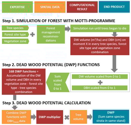
Figure 1.
Calculation of dead wood potential (DWP) was executed in three steps. First, simulations of forest growth produced the needed information of forest growth in 168 combinations of seven tree species, six forest site types, and four vegetation zones. Second, based on the previous information, altogether 168 different DWP functions were developed. Third, the spatial data of forest stands was converted into the DWP for each tree species with DWP functions. DW = dead wood, DBH = diameter at breast height, DBHmean = mean diameter at breast height.
As a first step, the data required for DWP modeling were simulated with the freely available Motti forest stand simulator (version 3.3) [40,41,42], provided by the Natural Resources Institute Finland. The functionality of the simulator is built upon NFI. Simulations provided data on the amount of dead wood (m3 per hectare) and diameter at breast height (DBH) of living trees (Figure 1, step 1). Simulations were made in 5-year intervals for 168 forest combinations of seven tree species (Alnus glutinosa ((L.) Gaertn.), Betula pendula (Roth), Betula pubescens (Ehrh.), Picea abies ((L.) H. Karst), Pinus sylvestris (L.), Populus tremula (L.), and other broadleaved tree species), six forest site types, and four vegetation zones from hemiboreal to northern boreal zones [43,44] (see Figure 2 and Appendix A for more details). Finnish forest management practice recommendations [45] set the guidelines for simulations. This information included, e.g., the number of seedlings per hectare and the timing of thinnings in a growing stand. No clear-cutting was executed in the simulations as stands were allowed to grow until the volume of the growing stock started to decline due to self-thinning effect. Simulations were executed on mineral soil only as simulations on peatland were not available in this version of Motti simulator. As the used version did not include information on the decomposition of dead wood, the volumes were larger than in reality. Based on expert opinion, the amounts of simulated dead wood were correct (considering the known deficiencies) and similar between tree species and forest site types. As the initial purpose for the modeling was to develop relative data on the probability of dead wood (differentiated from exact biological data) for spatial conservation prioritization needs, this was not seen as a problem.

Figure 2.
The map of Finland, the vegetation zones used in DWP modeling, and locations of the validation sites. The vegetation zones (grey lines) are as follows: I Southern Finland (vegetation zones 1 (hemiboreal), and 2a and 2c (southern boreal)), II Middle Finland (2b (southern boreal)), III Ostrobothnia and Kainuu (3a–c (middle boreal)), and IV Northern Finland (4a–d (northern boreal)). Southern (Evo) and northeastern (Kuhmo) sites are marked with pink squares.
The second step (Figure 1, Step 2) included the conversion of simulated estimates of dead wood and DBH into DWP functions. In total, 168 functions were formulated, one for each species–site type–vegetation zone combination (see Appendix A). This was done in four steps as described in Table 1. In Steps A and B, the amounts of dead wood (A) and DBH (B) were scaled between 0 and 1 in relation to the amount of them at the simulation maximum point, a point where the growing stock volume started to decline. In Step C, the scaled dead wood and the DBH were summed at each time step (minimum value 0 at time step 0, maximum value 2 at time step of 80 years in the example in Table 1). In Step D, the sum was rescaled from 0 to 1. These values were eventually used for fitting the DWP functions (Figure 3, Appendix A).

Table 1.
Example of construction of one dead wood potential (DWP) function. DWP function for other broadleaved trees in forest site type 1 (herb-rich forest) and in vegetation zone 2 (southern boreal 2b) was calculated as follows: Step A: the amount of dead wood was scaled between 0 and 1 in relation to the amount at the simulation maximum point (bolded). Step B: the DBH values were scaled similarly to the dead wood. Step C: the scaled dead wood and DBH were summed at each time step (min 0, max 2). Step D: this sum was rescaled from 0 to 1 forming DWP multiplier.
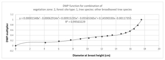
Figure 3.
Fitting the dead wood potential (DWP) functions and generating DWP multipliers. The figure describes one of the 168 functions, being the function for other broadleaved trees, growing in the most nutrient-rich soil (forest site type 1) in vegetation zone 2. DWP functions were formulated by fitting an 8-decimal function through the scaled DBH and dead wood values. Here, the X-axis is the diameter at breast height (DBH) and the Y-axis is the DWP multiplier for stratum volume. In this example the DWP multiplier for stratum volume for trees of, e.g., 10 cm mean diameter at breast height, is approximately 0.3.
Step 3 (Figure 1), required spatial forest stand data (DBHmean and volume per hectare) as at this point the DWP functions were used to convert the stand variables into the DWP. The DWP multiplier was defined with the DWP function using the stand DBHmean (Figure 3, Appendix A). Due to the overestimates that resulted from the extrapolation of the DWP functions, some of the DWP multipliers were unrealistically high. This was because natural forests host larger trees than commercial forests, especially for class other broadleaved trees. As we wanted to preserve the value of the large trees in natural forests, and on the other hand limit the overestimation of the DWP multiplier, its maximum was set to 2. Finally, the volume was multiplied with the DWP multiplier resulting in the DWP value. If there were more than one stratum of the same tree species in a stand, their DWP values were summed.
As an example, the stratum described in Figure 3 is Alnus incana ((L.) Moench) growing in herb-rich forests in the southern boreal zone. The DWP multiplier for DBHmean 10 cm is approximately 0.3. When the volume is 30 m3/ha, the DWP for this is:
where the DWP multiplier stands for the DWP function value at DBHmean of 10 cm (here 0.3). This is multiplied with the volume (i.e., 30 m3/ha) to achieve the DWP value 0.3 × 30 = 9.
2.2. Validation of DWP Modeling Method
The accuracy of the DWP modeling was validated on two separate sites in Finland, located in southern (Evo) and northeastern Finland (Kuhmo) (Figure 2). Both areas consist of managed and conserved boreal forests and are managed by Metsähallitus, the state-owned enterprise responsible for the management of state-owned areas. The most considerable differences between the areas, apart from vegetation zone, concern the management histories of the forests. Firstly, the Evo forest school, the oldest of the kind in Finland and still operational, has brought about systematic and intensive use and experimental research of forests for educational purposes in the Evo area. Secondly, throughout the history of the sites human population has been greater in southern Finland, inducing higher rates of forest utilization for self-sufficiency needs and later for private forestry [46].
The southern validation area was located in Hämeenlinna, in the Evo recreational forest area and in its surroundings (WGS84 lat: 63°52′, lon: 29°09′). Altogether, 100 field plots were measured during the summer 2018 of which 82 were in managed and 18 in conserved forest areas (Table 2). Almost half of the field plots (40 plots) were in forest stands that have been signed as habitats of special importance in terms of biodiversity or alike. On these habitats, forestry is practiced with limitations or not at all, but exact information is not publicly available [47,48,49]. Mineral soil covered 90 and peatland 10 of the plots [50].
Table 2.
Validation areas of Evo and Kuhmo in numbers.
In Evo, in total, 88 of the plots were allocated to different forest strata using inventory data provided by Metsähallitus. The area was divided into 100 theoretical strata according to the dominant tree species (pine, spruce, birch sp., aspen, and other deciduous), DBH class (0–10, 10–20, 20–30, 30–40, and 40–50 cm), and basal area class (0–15, 15–30, 30–45, and 45–60 m2/ha). In total, 51 of the theoretical strata were found from the site. The number of plots in each forest stratum was determined by the forest stands’ relative abundance in the study area. In addition, 12 field plots were positioned subjectively in areas where aspen (Populus tremula) was present. Plot-level DBHmean and mean volume were 24 cm and 260.4 m3/ha, and for dead trees 8 cm and 15.8 m3/ha, respectively (Table 3).
Table 3.
Plot-level characteristics for living and dead wood (DW) in the Evo validation area. DBHmean = mean diameter at breast height, H = mean height, Vol = volume, N = number of pieces, D = mean value of the dead wood diameters. Mean row indicates mean values for the whole area.
The northeastern validation area was in Kuhmo, covering the Hiidenportti National Park and Teerisuo-Lososuo Mire Reserve, and the commercially managed forests between them (WGS84 lat: 61°14′, lon: 25°07′). Here, 103 field plots were measured during the summer 2019 of which 44 were in managed and 59 in conserved forest areas (Table 2). Ten of the managed forest field plots were in forest stands with restricted utilization possibilities. Mineral soil covered 66 and peatland 37 of the plots. The plots were positioned using a systematic grid with 400 m distance between the neighboring plots in x and y directions. The plot-level DBHmean and mean volume were 18.5 cm and 117.6 m3/ha, and for dead trees 15.8 cm and 28.6 m3/ha, respectively (Table 4).
Table 4.
Plot-level characteristics for living and dead wood in the Kuhmo validation area.
In both validation areas, the field sample was measured as circular plots with a fixed radius of 9 m (or 5.64 m for trees with DBH < 4.5 cm). DBH and the tree species were determined for all living trees with a DBH of over 4.5 cm. For trees with a DBH of under 4.5 cm, only the height and number of the stems were recorded. Tree height was measured for 25% of trees in each forest stand stratum (i.e., for each tree species in both upper and lower canopy storey). The heights of individual trees were acquired by parametrizing Näslund’s height curve [51] using the measured sample trees. Tree volumes were calculated with taper curves [52].
Both standing and downed dead wood were measured in all plots. Standing and downed dead wood with a DBH of over 10 cm were measured for length and DBH (maximum diameter if breast height could not be defined). For fragments of dead wood, all pieces with a maximum diameter of 10 cm or more were recorded. For fallen trees, only the parts inside the plots were included in the inventory. For intact trunks, volumes were calculated with taper curves [52], whereas for snags and coarse woody debris, volume was derived using the formula of truncated cone. The species was determined for all dead wood whenever possible.
Plot-level attributes for living and dead wood were calculated for each stratum. Mean diameter was weighted with the basal area (Equation (2)), and for height value, Lorey’s mean height (Equation (3)) was used.
BA stands for tree-level basal area, DBH for diameter at breast height (i.e., 1.3 m), and h for tree height.
Information on the forest site type was taken from the Metsähallitus database [53,54].
The DWP conversion was carried out for Evo with functions from vegetation zone 1 and for Kuhmo with zone 3. Strata from the same tree species in the same forest stand were summed. For dead wood comparison, all DWPs in the same field plot were summed. This information was compared with the field measured amount of dead wood.
3. Results
The modeling method was validated on two separate areas in Finland (Figure 2) by comparing the reference volumes of dead wood to the modeled index values, i.e., DWP (Figure 4). The modeled DWP values were calculated based on field plot data that had been collected simultaneously with the dead wood data. Dead wood and DWP volumes of different tree species occurring in the same field plot were summed for the comparison. In Evo, the DWP values varied between 0 and 1623 (mean 132) and volume of dead wood from 0 to 320.2 m3 per hectare (mean 15.8). In Kuhmo, the DWP values ranged between 0 and 301 (mean 54) and dead wood volumes from 0 to 182.3 m3 per hectare (mean 28.6).
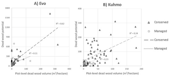
Figure 4.
Correlation between the dead wood potential (DWP) and dead wood volume in Evo and Kuhmo. The x-axis describes the plot level dead wood volume (m3 per hectare) and y-axis the DWP value for each plot. Both values are sums of different tree species in each plot. Plots on managed and conserved areas are marked with black triangles and gray circles, respectively. Coefficients of determinations are shown with dashed lines for managed and with dotted line for conserved field plots.
Results show that correlations between DWP and reference dead wood volumes (see Table 5) are more constant in Kuhmo than in Evo. When validation areas are observed separately, the correlation is stronger in Evo (R2 = 0.54) than in Kuhmo (R2 = 0.29). Correlation in conserved areas (strictly or with some degree of conservation) is stronger in Evo (R2 = 0.62) than in Kuhmo (R2 = 0.24). The results were investigated also based on soil type as the Motti simulations were executed only with mineral soil variables. Based on the results from Kuhmo, where 36% of field plots were on peatland, there were no significant differences between the correlations on different soil types (mineral soil and peatland both R2 = 0.24). As for Evo, where only 10% of field plots were on peatland, the correlation for mineral soil DWP was higher (R2 = 0.57) than for peatland (R2 = 0.30).
Table 5.
Coefficients of determinations for two validation sites. Total = all field plots on area, conserved = field plots in permanently protected areas and areas with restricted forest management, managed forests = field plots in non-conserved areas, mineral soil = field plots situated in mineral soil, and peatland = field plots in peatland.
In addition to plot-level validation, the DWP method was also examined on a larger scale using stand data for all forest stands in the Evo area managed by Metsähallitus [53,54,55]. The DWPs of different tree species were summed. The locations of areas known for their high biodiversity value and substantial dead wood volumes were revealed as shown in Figure 5.
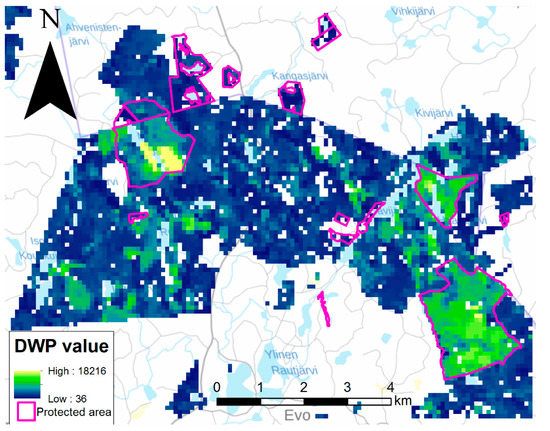
Figure 5.
Map of Evo validation area where tree stand data has been converted to dead wood potential (DWP) of each 96 × 96 m pixel. Protected forest areas are marked with pink borders. Only areas managed by Metsähallitus are included in this calculation.
4. Discussion
This article presents how forest stand information can be converted to wall-to-wall dead wood information that can be used for estimating forest biodiversity. In this approach, forest stand information (location, site type, tree species, DBHmean, and volume) was converted into the DWP by exploiting Motti forest simulations. Altogether, a process transforming stand data into DWP was generated to enable dead wood modeling for the whole of Finland or similar boreal ecosystems. The framework was validated with field data from two separate areas. The comparison between the DWP values and field data showed that the dead wood value of forests is predictable with our DWP modeling method. Additionally, the method recognized areas known for their substantial dead wood volumes, such as the protected areas of Kotinen and Sudenpesänkangas in Evo. Correlations between measured dead wood volume and modeled DWP varied between 0.11 and 0.62 indicating variation in reliability of the method between forest environments.
The results show that the performance of the DWP method varies depending on which field plots were examined. Differences within validation areas arise when comparing the correlations of managed and conserved plots in Evo (see Table 5), where the difference is evident. In managed forests the correlation between DWP and reference dead wood volume is low (R2 = 0.11), whereas in conserved areas the correlation was much higher (R2 = 0.62). This was expected as managed forests in Evo have been treated according to the present forest management standards, which increases the amount of growing stock but leaves very little dead wood on site. It is notable, that there were exceptionally big aspens (DBH > 50 cm) in some field plots in Evo, which resulted in significantly high DWPs (>600) for three of the plots as seen in Figure 4. When the correlations were examined without these three plots, the R2 values appeared similar to those in Kuhmo. In Evo, the R2 of all areas decreased from 0.54 to 0.24. The R2 of managed and conserved forests changed from 0.11 to 0.25 and from 0.62 to 0.28, respectively. However, as there were no measurement errors in these three plots, they were not seen as outliers but merely as an evidence of the influence of chance on the results. On the other hand, in Kuhmo the correlations were constant. A likely reason for this is the more homogeneous forest management practices, or merely the lack of them, as the Kuhmo area forms an ecologically important region, where only 33% of field plots were normally managed, 57% strictly conserved, and 10% conserved with an unknown degree of conservation. A similar phenomenon can also be found in other forest areas with softer management practices such as urban forests [13]. There were no exceptional field plots that would have stood out from others in Kuhmo, either. For comparison, in Evo, 42% of field plots were managed, 18% strictly conserved, and 40% conserved with an unknown degree of conservation. The low correlations can also be caused by the heterogeneity of forest environments in conserved areas. Conserved forest stands tend to differ from managed stands in terms of their vertical and horizontal structure, species distribution, and age structure [3,4].
When comparing the results between the validation areas, the correlations between DWP and reference dead wood volumes were higher in Evo (R2 = 0.54) than in Kuhmo (R2 = 0.29). As mentioned before, most of the difference is explained by the presence of big aspens in a few field plots. However, we would also like to bring up the possible impact of using the Motti simulator for calculating the default dead wood volumes for DWP models. As the Motti program is developed for forest growth modeling in managed forests, and forest management recommendations were used as input data for the simulations, the results should be more accurate in the widely managed area of Evo (only 18 field plots on conservation areas) than in the more pristine area of Kuhmo (59 field plots in conservation areas). Lastly, the occurrence of dead wood is very scattered in the landscape. Together with the small sample plot size (radius 9 m and area 252 m2), the scattered occurrence increases stochasticity of the data. To lower the influence of individual trees in the future, using bigger sample plots (e.g., 30 × 30 m) would likely decrease the variation between plots.
The starting point for this study was to find a method to be utilized for conversion of national stand-level forest data into information on biodiversity values. As the volume of trees was considered inadequate and expert opinion-based estimate too inaccurate, the openly available Motti program 3.3 was seen as a possibility as it had been developed to observe the effect of different management decisions on forest growth in a small scale based on Finnish NFI data. Ranius, Kindvall, Kruys, and Jonsson [23] simulated dead wood quantity for Picea abies ((L.) Karst.) including decomposition, but as for us, Motti provided a Finnish NFI-based ready-to-use platform for seven tree species. Other methods based on Finnish NFI were either designed for modeling the estimations of use of forests in more coarse resolution or the changes in dead wood rations and decomposition (see, e.g., [56,57]).
In general, the method presented in this paper provides a way to assess the biodiversity value of forests but also highlights the needs for development. The information and methodology on dead wood dynamics has increased during recent decades (see [22,57,58]), but accurate methods for locating dead wood, be it mapping or modeling, are still missing. As long as there are no techniques to measure dead wood automatically, modeling is needed. This DWP method should be improved first by adding dead wood dynamics into the calculations. Disturbances are an essential factor for the input rate of dead wood [59]. However, including natural disturbances, such as forest fires and windthrows, is challenging as long as operational stand-level data is pursued.
Decisions on the use of forest land are made daily. They are based on knowledge and values, and therefore it is essential to employ biodiversity data in decision making. This is especially because many nations, including Finland, have pledged to principles of sustainable development, Aichi targets, etc. [60]. As accurate landscape-level data on dead wood is often unavailable, DWP can be used to mimic such data. As forest management reduces biodiversity values but stimulates growth, thus increasing the DWP value, we recommend using DWP jointly with other datasets that can provide additional information on the conditions of the subject area (see also [23]). This can include information on threats to biodiversity (e.g., planning and construction), species observations (e.g., red-listed species), locations of permanently protected areas, former land use decisions (e.g., ditching or forest management), or forest heterogeneity (e.g., horizontal and vertical structure of forests, changes in bedrock, soil, or soil moisture). According to the preliminary results, the method has been used successfully for spatial conservation prioritization needs when used with additional data in Zonation analysis [36,61].
When the development of DWP modeling to achieve a national-level surrogate for biodiversity started, there were no open forest data nor interfaces to deliver such information. Nonetheless, the old method needed an update. In this study we presented a method that treats the whole of Finland equally and builds upon NFI data. Our method utilized simulation results, and 168 options for calculating biodiversity value were developed. The results show that DWP performs better in near-pristine southern forests known for their exceptionally good quality areas. These areas have high correlations with reference dead wood values. However, in northeastern areas with a history of softer management, the differences between the near-pristine and the managed forests is not as clear. As the forest management history affects the trees and the biodiversity values of the sites, we recommend using this data with supplementary data for estimating the site-specific biodiversity values.
5. Conclusions
Dead wood data is a key factor in the assessment of conservation values of forest areas. This DWP method provides a tool for assessing the dead wood potential of large forest areas when spatially accurate data on dead wood volume is unavailable. Considering the techniques and data sources available, the DWP method presented in this paper provides a potential tool for acquiring wall-to-wall dead wood data for landscape-level analysis.
Author Contributions
Conceptualization, N.M., N.L., P.H., A.L. and T.T.; formal analysis, N.M. and N.L.; investigation, N.M. and N.L.; methodology, N.M., N.L., P.H., A.L. and T.T.; software, N.L. and A.L.; supervision, P.H. and T.T.; validation, N.M., E.H. and T.T.; visualization, N.M.; writing—original draft, N.M., P.H. and T.T.; writing—review and editing, N.M., N.L., P.H. and T.T. All authors have read and agreed to the published version of the manuscript.
Funding
N.M., N.L. and A.L. were funded by the Finnish Ministry of the Environment (Forest Biodiversity Programme in Southern Finland METSO YM8/221/2010 and VN/6587/201). T.T. was funded by the Academy of Finland’s Strategic Research Council (IBC-Carbon, project number 312559). E.H. was funded from the LIFE financial instrument of the European Union (Beetles LIFE (LIFE17/NAT/FI/000181)). Open access funding was provided by University of Helsinki.
Acknowledgments
We would like to thank the rest of the people that have been involved in the developmental work of dead wood potential presented here: Tuomas Haapalehto and Marja Hokkanen (Metsähallitus Parks & Wildlife), Joona Lehtomäki (University of Helsinki), Kimmo Syrjänen (The Finnish Environment Institute), Saara Lilja-Rothsten and Lauri Saaristo (Tapio OY), and Tarja Wallenius, Jari Jämsen and Niklas Björkvist (Metsähallitus Forestry Inc.). We would also like to thank and all the people who collected field data, especially Aleksi Ritakallio and Pasi Korpelainen. Lastly, we would like to express our gratitude to Sonja Virta for her linguistic help with the manuscript.
Conflicts of Interest
The authors declare no conflict of interest. The funders had no role in the design of the study; in the collection, analyses, or interpretation of data; in the writing of the manuscript, or in the decision to publish the results.
Appendix A
Dead Wood Potential (DWP) Functions
These 168 DWP functions were used for calculating the DWP for every tree stratum. X in functions was replaced with stratum DBHmean, which gave the DWP multiplier for stratum volume as an outcome. All multipliers greater than 2 is recommended to set to 2.
The vegetations zones were (1) hemiboreal 1 and southern boreal 2a and 2c, (2) southern boreal 2b, (3) middle boreal 3a–c (4) northern boreal 4a–d [42,43]. The forest site types (mineral ground forest site types and their counterparts on peatland) were (1) herb rich forests, (2) herb-rich heath forest, (3) mesic heath forest, (4) sub-xeric heath forest, (5) xeric heath forest, and (6) barren heath forest. The forest site types 7, 8, and 9 (the most barren ones) were calculated with functions for barren heath forest (6). The DBH value in the table Appendix A is the value of DBH in Motti simulation maximum for tree volume in that tree species–vegetation zone–forest site type combination.
| Tree Species | Vegetation Zone | Forest Site Type | Functions for Dead Wood Potential (DWP) Calculation | DBH (cm) | |
| 1 | Picea abies ((L.) H. Karst.) | 1 | Herb-rich forest | y = 0.0000000161x5 − 0.0000017284x4 + 0.0000659861x3 − 0.0010311017x2 + 0.0147885592x − 0.0049002034 | 55.4 |
| 2 | Picea abies | 1 | Herb-rich heath forest | y = 0.0000000184x5 − 0.0000017033x4 + 0.0000563171x3 − 0.0007552955x2 + 0.0134742452x − 0.0023702218 | 50.7 |
| 3 | Picea abies | 1 | Mesic heath forest | y = 0.0000005264x4 − 0.0000425948x3 + 0.0011372754x2 − 0.0002934437x + 0.0169174344 | 52.6 |
| 4 | Picea abies | 1 | Sub-xeric heath forest | y = 0.0000005986x4 − 0.0000192421x3 + 0.0003016817x2 + 0.0115485958x + 0.0025994013 | 37 |
| 5 | Picea abies | 1 | Xeric heath forest | y = 0.0000002716x5 − 0.0000157163x4 + 0.0003436485x3 − 0.0030953347x2 + 0.0272649678x − 0.0038273867 | 28.8 |
| 6 | Picea abies | 1 | Barren heath forest | y = 0.0010125092x2 + 0.0150097643x + 0.0023813648 | 25 |
| 7 | Picea abies | 2 | Herb-rich forest | y = 0.0000006155x4 − 0.0000450509x3 + 0.0010562901x2 + 0.0018961460x + 0.0096330860 | 53.5 |
| 8 | Picea abies | 2 | Herb-rich heath forest | y = 0.0000006155x4 − 0.0000450509x3 + 0.0010562901x2 + 0.0018961460x + 0.0096330860 | 50.7 |
| 9 | Picea abies | 2 | Mesic heath forest | y = 0.0000005306x4 − 0.0000448023x3 + 0.0012362144x2 − 0.0014654573x + 0.0164931209 | 53.7 |
| 10 | Picea abies | 2 | Sub-xeric heath forest | y = 0.0000013384x4 − 0.0000816544x3 + 0.0017079190x2 + 0.0008330889x + 0.0132025288 | 40 |
| 11 | Picea abies | 2 | Xeric heath forest | y = 0.0000040479x4 − 0.0001761466x3 + 0.0027120941x2 + 0.0028549025x + 0.0111397051 | 29.3 |
| 12 | Picea abies | 2 | Barren heath forest | y = 0.0000092054x4 − 0.0003755234x3 + 0.0052546605x2 − 0.0051711784x + 0.0160875537 | 25.5 |
| 13 | Picea abies | 3 | Herb-rich forest | y = 0.0000122709x3 − 0.0007624465x2 + 0.0290175225x − 0.0309302578 | 48.3 |
| 14 | Picea abies | 3 | Herb-rich heath forest | y = 0.0000000372x5 − 0.0000032919x4 + 0.0001048535x3 − 0.0013661297x2 + 0.0173523584x − 0.0041851545 | 45.6 |
| 15 | Picea abies | 3 | Mesic heath forest | y = 0.0000008241x4 − 0.0000591222x3 + 0.0014262304x2 − 0.0001559167x + 0.0149484085 | 46.2 |
| 16 | Picea abies | 3 | Sub-xeric heath forest | y = 0.0000018927x4 − 0.0000772079x3 + 0.0012286067x2 + 0.0087162361x + 0.0067653140 | 31.8 |
| 17 | Picea abies | 3 | Xeric heath forest | y = 0.0000007434x5 − 0.0000389231x4 + 0.0007562472x3 − 0.0060387418x2 + 0.0369600166x − 0.0055048664 | 24.8 |
| 18 | Picea abies | 3 | Barren heath forest | y = 0.0000018814x5 − 0.0000895617x4 + 0.0015570974x3 − 0.0110989030x2 + 0.0500584897x − 0.0068869694 | 21.8 |
| 19 | Picea abies | 4 | Herb-rich forest | y = 0.0000001362x5 − 0.0000089326x4 + 0.0002173264x3 − 0.0021928022x2 + 0.0227845402x − 0.0043775857 | 33.7 |
| 20 | Picea abies | 4 | Herb-rich heath forest | y = 0.0000049058x4 − 0.0002520313x3 + 0.0043429636x2 − 0.0095134968x + 0.0253623319 | 31.3 |
| 21 | Picea abies | 4 | Mesic heath forest | y = 0.0000038422x4 − 0.0001752678x3 + 0.0028749856x2 + 0.0007796390x + 0.0148666980 | 29.8 |
| 22 | Picea abies | 4 | Sub-xeric heath forest | y = 0.0000015843x5 − 0.0000734457x4 + 0.0012755734x3 − 0.0091984010x2 + 0.0464506582x − 0.0076350317 | 21.4 |
| 23 | Picea abies | 4 | Xeric heath forest | y = 0.0000050816x5 − 0.0001963719x4 + 0.0028507686x3 − 0.0173939950x2 + 0.0655229900x − 0.0088755793 | 17.4 |
| 24 | Picea abies | 4 | Barren heath forest | y = 0.0000000094x5 − 0.0000016212x4 + 0.0001104195x3 − 0.0035850719x2 + 0.0628358948x − 0.0934533866 | 15.6 |
| 25 | Pinus sylvestris (L.) | 1 | Herb-rich forest | y = 0.0000004623x4 − 0.0000222413x3 + 0.0001927273x2 + 0.0120210416x − 0.0075600744 | 48.3 |
| 26 | Pinus sylvestris | 1 | Herb-rich heath forest | y = 0.0000000098x5 + 0.0000001796x4 − 0.0000515518x3 + 0.0015055128x2 − 0.0006701712x + 0.0042664418 | 46.7 |
| 27 | Pinus sylvestris | 1 | Mesic heath forest | y = 0.0000013512x4 − 0.0001013567x3 + 0.0023850056x2 − 0.0060850485x + 0.0064301561 | 46.7 |
| 28 | Pinus sylvestris | 1 | Sub-xeric heath forest | y = 0.0000012252x4 − 0.0000893534x3 + 0.0021243604x2 − 0.0042316368x + 0.0101178798 | 45.1 |
| 29 | Pinus sylvestris | 1 | Xeric heath forest | y = 0.0000012644x4 − 0.0000693070x3 + 0.0010995711x2 + 0.0077363288x − 0.0045700136 | 41.8 |
| 30 | Pinus sylvestris | 1 | Barren heath forest | y = 0.0000000283x5 + 0.0000006755x4 − 0.0001089991x3 + 0.0024651722x2 − 0.0018870714x + 0.0052463026 | 37.1 |
| 31 | Pinus sylvestris | 2 | Herb-rich forest | y = 0.0000009335x4 − 0.0000663941x3 + 0.0014401761x2 + 0.0015466061x + 0.0000349890 | 48.3 |
| 32 | Pinus sylvestris | 2 | Herb-rich heath forest | y = 0.0000006174x4 − 0.0000326284x3 + 0.0004487432x2 + 0.0105988127x − 0.0075041933 | 46.2 |
| 33 | Pinus sylvestris | 2 | Mesic heath forest | y = 0.0000229170x3 − 0.0010204842x2 + 0.0216302498x − 0.0105496624 | 45.7 |
| 34 | Pinus sylvestris | 2 | Sub-xeric heath forest | y = 0.0000010166x4 − 0.0000676667x3 + 0.0014820782x2 + 0.0015167476x + 0.0046006516 | 44.3 |
| 35 | Pinus sylvestris | 2 | Xeric heath forest | y = 0.0000020094x4 − 0.0001301944x3 + 0.0026234281x2 − 0.0040767151x + 0.0070796259 | 41.7 |
| 36 | Pinus sylvestris | 2 | Barren heath forest | y = 0.0000030626x4 − 0.0001696886x3 + 0.0029412809x2 − 0.0017420282x + 0.0028058062 | 36.5 |
| 37 | Pinus sylvestris | 3 | Herb-rich forest | y = 0.0000003836x4 − 0.0000136713x3 − 0.0000543905x2 + 0.0147055443x − 0.0115382974 | 47.2 |
| 38 | Pinus sylvestris | 3 | Herb-rich heath forest | y = 0.0000000581x5 − 0.0000047820x4 + 0.0001280600x3 − 0.0011291177x2 + 0.0132446600x + 0.0021001166 | 44.6 |
| 39 | Pinus sylvestris | 3 | Mesic heath forest | y = 0.0000005446x4 − 0.0000164774x3 − 0.0001563580x2 + 0.0170326122x − 0.0151731205 | 43.7 |
| 40 | Pinus sylvestris | 3 | Sub-xeric heath forest | y = 0.0000012675x4 − 0.0000882199x3 + 0.0020954396x2 − 0.0031922096x + 0.0113978403 | 42.2 |
| 41 | Pinus sylvestris | 3 | Xeric heath forest | y = 0.0000000485x5 − 0.0000019886x4 − 0.0000093689x3 + 0.0010724885x2 + 0.0036876387x + 0.0065684616 | 39.3 |
| 42 | Pinus sylvestris | 3 | Barren heath forest | y = 0.0000003745x5 − 0.0000274009x4 + 0.0007016601x3 − 0.0072645366x2 + 0.0404266958x − 0.0025942599 | 34.5 |
| 43 | Pinus sylvestris | 4 | Herb-rich forest | y = 0.0000201272x3 − 0.0007666773x2 + 0.0187609364x − 0.0056661884 | 43.7 |
| 44 | Pinus sylvestris | 4 | Herb-rich heath forest | y = 0.0000225723x3 − 0.0006202513x2 + 0.0177580701x − 0.0011832482 | 38.1 |
| 45 | Pinus sylvestris | 4 | Mesic heath forest | y = 0.0000127058x3 + 0.0001898738x2 + 0.0042006395x + 0.0443521300 | 36 |
| 46 | Pinus sylvestris | 4 | Sub-xeric heath forest | y = 0.0000116647x3 + 0.0000042624x2 + 0.0117378253x + 0.0070122178 | 36.3 |
| 47 | Pinus sylvestris | 4 | Xeric heath forest | y = 0.0000038240x4 − 0.0001528377x3 + 0.0019583311x2 + 0.0093019582x − 0.0011384075 | 30.2 |
| 48 | Pinus sylvestris | 4 | Barren heath forest | y = 0.0000759311x3 − 0.0018448651x2 + 0.0292579425x − 0.0051270841 | 27.8 |
| 49 | Betula pendula (Roth) | 1 | Herb-rich forest | y = 0.0000000698x5 − 0.0000029907x4 + 0.0000126208x3 + 0.0006443447x2 + 0.0081154853x + 0.0028446742 | 36.8 |
| 50 | Betula pendula | 1 | Herb-rich heath forest | y = 0.0000004286x5 − 0.0000315153x4 + 0.0008107264x3 − 0.0084532404x2 + 0.0439597902x − 0.0043918714 | 34.5 |
| 51 | Betula pendula | 1 | Mesic heath forest | y = 0.0000004916x5 − 0.0000342620x4 + 0.0008300406x3 − 0.0080614969x2 + 0.0409280753x − 0.0062904828 | 33.1 |
| 52 | Betula pendula | 1 | Sub-xeric heath forest | y = 0.0000848874x3 − 0.0025538279x2 + 0.0357856249x − 0.0197727664 | 29.7 |
| 53 | Betula pendula | 1 | Xeric heath forest | y = 0.0000026167x5 − 0.0000929878x4 + 0.0011342487x3 − 0.0054258503x2 + 0.0332693801x + 0.0003155131 | 19.8 |
| 54 | Betula pendula | 1 | Barren heath forest | y = 0.0000124704x5 − 0.0004611922x4 + 0.0060537298x3 − 0.0328496818x2 + 0.0907612742x − 0.0041143955 | 17 |
| 55 | Betula pendula | 2 | Herb-rich forest | y = 0.0000023886x4 − 0.0001199093x3 + 0.0017604835x2 + 0.0064533491x + 0.0003928322 | 36.8 |
| 56 | Betula pendula | 2 | Herb-rich heath forest | y = 0.0000001835x5 − 0.0000111267x4 + 0.0002244220x3 − 0.0016810971x2 + 0.0179017119x + 0.0010852197 | 34.4 |
| 57 | Betula pendula | 2 | Mesic heath forest | y = 0.0000006281x5 − 0.0000454954x4 + 0.0011532698x3 − 0.0118540667x2 + 0.0561558320x − 0.0080901647 | 33 |
| 58 | Betula pendula | 2 | Sub-xeric heath forest | y = 0.0000800245x3 − 0.0022774568x2 + 0.0326993896x − 0.0144578193 | 29.5 |
| 59 | Betula pendula | 2 | Xeric heath forest | y = 0.0000041677x5 − 0.0001574013x4 + 0.0020859079x3 − 0.0112566189x2 + 0.0463268449x − 0.0010374605 | 19.3 |
| 60 | Betula pendula | 2 | Barren heath forest | y = 0.0000129718x5 − 0.0004756278x4 + 0.0061959914x3 − 0.0334149409x2 + 0.0918745245x − 0.0041449752 | 16.8 |
| 61 | Betula pendula | 3 | Herb-rich forest | y = 0.0000000812x5 − 0.0000025757x4 − 0.0000173798x3 + 0.0010223015x2 + 0.0081035278x + 0.0043284919 | 34.1 |
| 62 | Betula pendula | 3 | Herb-rich heath forest | y = 0.0000007434x5 − 0.0000509956x4 + 0.0012244189x3 − 0.0119180632x2 + 0.0550499985x − 0.0089540976 | 31.4 |
| 63 | Betula pendula | 3 | Mesic heath forest | y = 0.0000044906x4 − 0.0001489538x3 + 0.0013133137x2 + 0.0156569208x − 0.0038277485 | 28.6 |
| 64 | Betula pendula | 3 | Sub-xeric heath forest | y = 0.0000843469x3 − 0.0014555367x2 + 0.0237551975x + 0.0050821260 | 25.2 |
| 65 | Betula pendula | 3 | Xeric heath forest | y = 0.0000134762x5 − 0.0004836110x4 + 0.0061431121x3 − 0.0320798098x2 + 0.0873219905x − 0.0061012210 | 16.6 |
| 66 | Betula pendula | 3 | Barren heath forest | y = 0.0000276450x5 − 0.0008898351x4 + 0.0101340238x3 − 0.0473476725x2 + 0.1086884842x − 0.0051200733 | 14.7 |
| 67 | Betula pendula | 4 | Herb-rich forest | y = 0.0000142294x3 + 0.0006851383x2 + 0.0038379153x + 0.0305639777 | 28.5 |
| 68 | Betula pendula | 4 | Herb-rich heath forest | y = 0.0000821947x3 − 0.0013489222x2 + 0.0225653406x + 0.0086468736 | 25.2 |
| 69 | Betula pendula | 4 | Mesic heath forest | y = 0.0001487373x3 − 0.0032477261x2 + 0.0384672973x − 0.0112808847 | 23.5 |
| 70 | Betula pendula | 4 | Sub-xeric heath forest | y = 0.0000237811x4 − 0.0006969965x3 + 0.0063541234x2 + 0.0058201682x + 0.0066524128 | 20.7 |
| 71 | Betula pendula | 4 | Xeric heath forest | y = 0.0000341585x5 − 0.0010567167x4 + 0.0115821628x3 − 0.0522670867x2 + 0.1164330642x − 0.0110599387 | 14.1 |
| 72 | Betula pendula | 4 | Barren heath forest | y = 0.0000607977x5 − 0.0017280977x4 + 0.0173812267x3 − 0.0718177791x2 + 0.1399870537x − 0.0109816278 | 12.8 |
| 73 | Betula pubescens (Ehrh.) | 1 | Herb-rich forest | y = 0.0000005147x5 − 0.0000397530x4 + 0.0010706348x3 − 0.0116114394x2 + 0.0563842058x − 0.0081785677 | 34.6 |
| 74 | Betula pubescens | 1 | Herb-rich heath forest | y = 0.0000008478x5 − 0.0000578998x4 + 0.0013844346x3 − 0.0134123160x2 + 0.0598250568x − 0.0064807858 | 30.8 |
| 75 | Betula pubescens | 1 | Mesic heath forest | y = 0.0000008494x5 − 0.0000570531x4 + 0.0013427466x3 − 0.0128234040x2 + 0.0577501024x − 0.0077276424 | 30.4 |
| 76 | Betula pubescens | 1 | Sub-xeric heath forest | y = 0.0000011998x5 − 0.0000697299x4 + 0.0014158143x3 − 0.0115995601x2 + 0.0505531563x − 0.0090827056 | 27.2 |
| 77 | Betula pubescens | 1 | Xeric heath forest | y = 0.0000195064x5 − 0.0006349216x4 + 0.0073406555x3 − 0.0351181493x2 + 0.0908986831x − 0.0032060826 | 15.2 |
| 78 | Betula pubescens | 1 | Barren heath forest | y = 0.0000016683x5 − 0.0000969083x4 + 0.0021895457x3 − 0.0235631730x2 + 0.1367625836x − 0.1076733924 | 13.2 |
| 79 | Betula pubescens | 2 | Herb-rich forest | y = 0.0000005078x5 − 0.0000396260x4 + 0.0010777939x3 − 0.0118120982x2 + 0.0575682212x − 0.0096812959 | 34.9 |
| 80 | Betula pubescens | 2 | Herb-rich heath forest | y = 0.0000007892x5 − 0.0000545302x4 + 0.0013190001x3 − 0.0129279489x2 + 0.0586627985x − 0.0068225071 | 31.1 |
| 81 | Betula pubescens | 2 | Mesic heath forest | y = 0.0000009307x5 − 0.0000626945x4 + 0.0014860637x3 − 0.0143806824x2 + 0.0637802760x − 0.0046716255 | 30.1 |
| 82 | Betula pubescens | 2 | Sub-xeric heath forest | y = 0.0000013047x5 − 0.0000748816x4 + 0.0015031182x3 − 0.0121962798x2 + 0.0522196363x − 0.0092041945 | 26.8 |
| 83 | Betula pubescens | 2 | Xeric heath forest | y = 0.0000199097x5 − 0.0006442758x4 + 0.0074117015x3 − 0.0353237563x2 + 0.0913360115x − 0.0032317430 | 15.1 |
| 84 | Betula pubescens | 2 | Barren heath forest | y = 0.0000434301x5 − 0.0012348638x4 + 0.0125008008x3 − 0.0525099819x2 + 0.1142383729x − 0.0022700043 | 13.1 |
| 85 | Betula pubescens | 3 | Herb-rich forest | y = 0.0000008926x5 − 0.0000586134x4 + 0.0013438732x3 − 0.0124500644x2 + 0.0553706773x − 0.0088025839 | 30.1 |
| 86 | Betula pubescens | 3 | Herb-rich heath forest | y = 0.0000011983x5 − 0.0000734126x4 + 0.0015788582x3 − 0.0138170861x2 + 0.0589918348x − 0.0079444343 | 27.9 |
| 87 | Betula pubescens | 3 | Mesic heath forest | y = 0.0000024729x5 − 0.0001290246x4 + 0.0023699864x3 − 0.0177546791x2 + 0.0658269113x − 0.0055008469 | 23.9 |
| 88 | Betula pubescens | 3 | Sub-xeric heath forest | y = 0.0003131284x3 − 0.0068869653x2 + 0.0632760365x − 0.0340467609 | 20 |
| 89 | Betula pubescens | 3 | Xeric heath forest | y = 0.0000469941x5 − 0.0013264440x4 + 0.0132503785x3 − 0.0542358803x2 + 0.1129146343x − 0.0040491170 | 13 |
| 90 | Betula pubescens | 3 | Barren heath forest | y = 0.0000973178x5 − 0.0024765182x4 + 0.0223414139x3 − 0.0827234057x2 + 0.1457634078x − 0.0033752688 | 11.5 |
| 91 | Betula pubescens | 4 | Herb-rich forest | y = 0.0001056533x3 − 0.0018595467x2 + 0.0276357197x + 0.0014319387 | 23.7 |
| 92 | Betula pubescens | 4 | Herb-rich heath forest | y = 0.0000135491x4 − 0.0002887099x3 + 0.0014516350x2 + 0.0247671329x − 0.0038273969 | 20.5 |
| 93 | Betula pubescens | 4 | Mesic heath forest | y = 0.0000520241x4 − 0.0015190382x3 + 0.0140511857x2 − 0.0150064164x + 0.0165457552 | 18.4 |
| 94 | Betula pubescens | 4 | Sub-xeric heath forest | y = 0.0000946763x4 − 0.0025073073x3 + 0.0211413109x2 − 0.0274326999x + 0.0237633916 | 16.1 |
| 95 | Betula pubescens | 4 | Xeric heath forest | y = 0.0001112251x5 − 0.0027012577x4 + 0.0231219019x3 − 0.0808900733x2 + 0.1407658016x − 0.0085794462 | 11.1 |
| 96 | Betula pubescens | 4 | Barren heath forest | y = 0.0002010279x5 − 0.0045434558x4 + 0.0360747028x3 − 0.1164661501x2 + 0.1750207637x − 0.0087745744 | 10.2 |
| 97 | Populus tremula (L.) | 1 | Herb-rich forest | y = 0.0000004911x5 − 0.0000364224x4 + 0.0009463543x3 − 0.0099537068x2 + 0.0497723271x − 0.0052573545 | 33.7 |
| 98 | Populus tremula | 1 | Herb-rich heath forest | y = 0.0000006389x5 − 0.0000448857x4 + 0.0011066815x3 − 0.0110807294x2 + 0.0529277624x − 0.0053017914 | 31.9 |
| 99 | Populus tremula | 1 | Mesic heath forest | y = 0.0000079795x4 − 0.0004296518x3 + 0.0072278336x2 − 0.0222549155x + 0.0216449596 | 31.4 |
| 100 | Populus tremula | 1 | Sub-xeric heath forest | y = 0.0000025340x5 − 0.0001252167x4 + 0.0021839468x3 − 0.0155782893x2 + 0.0596280231x − 0.0065490851 | 23 |
| 101 | Populus tremula | 1 | Xeric heath forest | y = 0.0000113631x5 − 0.0004077298x4 + 0.0051975367x3 − 0.0273533659x2 + 0.0790810564x − 0.0031555977 | 16.8 |
| 102 | Populus tremula | 1 | Barren heath forest | y = 0.0000233258x5 − 0.0007620291x4 + 0.0088408222x3 − 0.0423768934x2 + 0.1028515013x − 0.0028496552 | 15 |
| 103 | Populus tremula | 2 | Herb-rich forest | y = 0.0000004952x5 − 0.0000373045x4 + 0.0009829351x3 − 0.0104664729x2 + 0.0520280776x − 0.0067635479 | 34 |
| 104 | Populus tremula | 2 | Herb-rich heath forest | y = 0.0000005734x5 − 0.0000429847x4 + 0.0011286691x3 − 0.0120179552x2 + 0.0581328449x − 0.0081317520 | 33.5 |
| 105 | Populus tremula | 2 | Mesic heath forest | y = 0.0000084733x4 − 0.0004459214x3 + 0.0073424690x2 − 0.0218166161x + 0.0214580688 | 30.8 |
| 106 | Populus tremula | 2 | Sub-xeric heath forest | y = 0.0000026447x5 − 0.0001281296x4 + 0.0021927625x3 − 0.0153685162x2 + 0.0588012658x − 0.0058806919 | 22.7 |
| 107 | Populus tremula | 2 | Xeric heath forest | y = 0.0000108433x5 − 0.0003926531x4 + 0.0050555795x3 − 0.0269215264x2 + 0.0788169919x − 0.0034048924 | 17 |
| 108 | Populus tremula | 2 | Barren heath forest | y = 0.0000245697x5 − 0.0007935809x4 + 0.0091121621x3 − 0.0432970898x2 + 0.1043628446x − 0.0028581742 | 14.8 |
| 109 | Populus tremula | 3 | Herb-rich forest | y = 0.0000005817x5 − 0.0000388786x4 + 0.0009104427x3 − 0.0086232657x2 + 0.0433743113x − 0.0060358705 | 31.2 |
| 110 | Populus tremula | 3 | Herb-rich heath forest | y = 0.0000008455x5 − 0.0000541241x4 + 0.0012171283x3 − 0.0111218403x2 + 0.0512982223x − 0.0068051191 | 29.4 |
| 111 | Populus tremula | 3 | Mesic heath forest | y = 0.0001562745x3 − 0.0046067531x2 + 0.0537072162x − 0.0412866515 | 26 |
| 112 | Populus tremula | 3 | Sub-xeric heath forest | y = 0.0003543187x3 − 0.0078771000x2 + 0.0700779711x − 0.0376300965 | 19.6 |
| 113 | Populus tremula | 3 | Xeric heath forest | y = 0.0000206683x5 − 0.0006761866x4 + 0.0078290083x3 − 0.0371976946x2 + 0.0928146663x − 0.0049042456 | 15.2 |
| 114 | Populus tremula | 3 | Barren heath forest | y = 0.0000439513x5 − 0.0012918402x4 + 0.0134394830x3 − 0.0573061683x2 + 0.1192271055x − 0.0040964012 | 13.4 |
| 115 | Populus tremula | 4 | Herb-rich forest | y = 0.0000048016x4 − 0.0001117991x3 + 0.0003543209x2 + 0.0226836786x − 0.0063111968 | 25.8 |
| 116 | Populus tremula | 4 | Herb-rich heath forest | y = 0.0000919159x3 − 0.0013406533x2 + 0.0229964151x + 0.0086222734 | 23.7 |
| 117 | Populus tremula | 4 | Mesic heath forest | y = 0.0001862663x3 − 0.0038237204x2 + 0.0422245854x − 0.0127054555 | 21.8 |
| 118 | Populus tremula | 4 | Sub-xeric heath forest | y = 0.0000116611x5 − 0.0003967235x4 + 0.0047990655x3 − 0.0240006334x2 + 0.0726713154x − 0.0077883137 | 16.3 |
| 119 | Populus tremula | 4 | Xeric heath forest | y = 0.0000449284x5 − 0.0013038827x4 + 0.0133998791x3 − 0.0566353526x2 + 0.1195635316x − 0.0100572770 | 13.3 |
| 120 | Populus tremula | 4 | Barren heath forest | y = 0.0000843400x5 − 0.0022248614x4 + 0.0207460282x3 − 0.0793170088x2 + 0.1446013272x − 0.0096399207 | 11.9 |
| 121 | Alnus glutinosa ((L.) Gaertn.) | 1 | Herb-rich forest | y = 0.0000074496x5 − 0.0003525090x4 + 0.0059404760x3 − 0.0415701978x2 + 0.1244785725x − 0.0023168716 | 20.5 |
| 122 | Alnus glutinosa | 1 | Herb-rich heath forest | y = 0.0000128704x5 − 0.0005507459x4 + 0.0084512065x3 − 0.0543659749x2 + 0.1493117306x − 0.0015781598 | 18.3 |
| 123 | Alnus glutinosa | 1 | Mesic heath forest | y = 0.0000120440x5 − 0.0004985693x4 + 0.0073668242x3 − 0.0453107979x2 + 0.1239013027x − 0.0021327974 | 18.1 |
| 124 | Alnus glutinosa | 1 | Sub-xeric heath forest | y = 0.0000988573x5 − 0.0026154349x4 + 0.0245845858x3 − 0.0956244366x2 + 0.1696714860x − 0.0020026933 | 11.8 |
| 125 | Alnus glutinosa | 1 | Xeric heath forest | y = 0.0004043769x5 − 0.0089613217x4 + 0.0712133327x3 − 0.2367022954x2 + 0.3241998142x − 0.0006634528 | 9.37 |
| 126 | Alnus glutinosa | 1 | Barren heath forest | y = 0.0053924930x3 − 0.0590984236x2 + 0.2201961376x − 0.0256368371 | 8.4 |
| 127 | Alnus glutinosa | 2 | Herb-rich forest | y = 0.0000075081x5 − 0.0003506327x4 + 0.0058294432x3 − 0.0402069148x2 + 0.1199446382x − 0.0026136340 | 20.3 |
| 128 | Alnus glutinosa | 2 | Herb-rich heath forest | y = 0.0000145047x5 − 0.0006014285x4 + 0.0089383388x3 − 0.0556707462x2 + 0.1490098749x − 0.0016618983 | 17.8 |
| 129 | Alnus glutinosa | 2 | Mesic heath forest | y = 0.0000132149x5 − 0.0005805631x4 + 0.0091730318x3 − 0.0610986544x2 + 0.1701848768x − 0.0011818426 | 18.5 |
| 130 | Alnus glutinosa | 2 | Sub-xeric heath forest | y = 0.0019794703x3 − 0.0307260916x2 + 0.1574728842x − 0.0118975512 | 12 |
| 131 | Alnus glutinosa | 2 | Xeric heath forest | y = 0.0004318896x5 − 0.0094351732x4 + 0.0739824124x3 − 0.2429702683x2 + 0.3295543992x − 0.0006597002 | 9.23 |
| 132 | Alnus glutinosa | 2 | Barren heath forest | y = 0.0057173199x3 − 0.0617247899x2 + 0.2259910364x − 0.0255182941 | 8.26 |
| 133 | Alnus glutinosa | 3 | Herb-rich forest | y = 0.0000082551x5 − 0.0003559860x4 + 0.0054499415x3 − 0.0344546810x2 + 0.1004627207x − 0.0032690688 | 19.2 |
| 134 | Alnus glutinosa | 3 | Herb-rich heath forest | y = 0.0000141998x5 − 0.0005663320x4 + 0.0080472709x3 − 0.0475170982x2 + 0.1254229615x − 0.0030199959 | 17.5 |
| 135 | Alnus glutinosa | 3 | Mesic heath forest | y = 0.0000162769x5 − 0.0005859380x4 + 0.0075014554x3 − 0.0397237899x2 + 0.1025931440x − 0.0025992132 | 16.3 |
| 136 | Alnus glutinosa | 3 | Sub-xeric heath forest | y = 0.0001040101x5 − 0.0027123121x4 + 0.0250222206x3 − 0.0946173574x2 + 0.1625612077x − 0.0038541966 | 11.6 |
| 137 | Alnus glutinosa | 3 | Xeric heath forest | y = 0.0003465269x5 − 0.0075489957x4 + 0.0583114029x3 − 0.1852030100x2 + 0.2496181502x − 0.0024301401 | 9.47 |
| 138 | Alnus glutinosa | 3 | Barren heath forest | y = 0.0006307148x5 − 0.0127831695x4 + 0.0918602416x3 − 0.2716487035x2 + 0.3275330978x − 0.0017410250 | 8.66 |
| 139 | Alnus glutinosa | 4 | Herb-rich forest | y = 0.0000109015x5 − 0.0004002291x4 + 0.0052118785x3 − 0.0279047711x2 + 0.0799147601x − 0.0042342366 | 17.1 |
| 140 | Alnus glutinosa | 4 | Herb-rich heath forest | y = 0.0000232563x5 − 0.0007786065x4 + 0.0092497879x3 − 0.0451945856x2 + 0.1074552414x − 0.0040762029 | 15.2 |
| 141 | Alnus glutinosa | 4 | Mesic heath forest | y = 0.0000222440x5 − 0.0007248221x4 + 0.0083510986x3 − 0.0394504590x2 + 0.0966699136x − 0.0079985370 | 15 |
| 142 | Alnus glutinosa | 4 | Sub-xeric heath forest | y = 0.0001195714x5 − 0.0029180046x4 + 0.0250762833x3 − 0.0880100258x2 + 0.1496041466x − 0.0094044374 | 11.1 |
| 143 | Alnus glutinosa | 4 | Xeric heath forest | y = 0.0003526446x5 − 0.0074890484x4 + 0.0557315217x3 − 0.1679583885x2 + 0.2211855538x − 0.0091879247 | 9.41 |
| 144 | Alnus glutinosa | 4 | Barren heath forest | y = 0.0049165839x3 − 0.0569047042x2 + 0.2187235843x − 0.0565417242 | 8.77 |
| 145 | Other broadleaved | 1 | Herb-rich forest | y = 0.0000159331x5 − 0.0006551323x4 + 0.0096463222x3 − 0.0594495816x2 + 0.1557082599x − 0.0009990372 | 17.6 |
| 146 | Other broadleaved | 1 | Herb-rich heath forest | y = 0.0000205100x5 − 0.0007254342x4 + 0.0093421540x3 − 0.0512173513x2 + 0.1319081391x − 0.0004774367 | 15.4 |
| 147 | Other broadleaved | 1 | Mesic heath forest | y = 0.0000401044x5 − 0.0013620237x4 + 0.0166251208x3 − 0.0854673359x2 + 0.1885573057x − 0.0007201616 | 14.6 |
| 148 | Other broadleaved | 1 | Sub-xeric heath forest | y = 0.0002650248x5 − 0.0060471431x4 + 0.0492898767x3 − 0.1672909525x2 + 0.2451454027x − 0.0006349294 | 9.91 |
| 149 | Other broadleaved | 1 | Xeric heath forest | y = 0.0026390485x4 − 0.0378261877x3 + 0.1704826425x2 − 0.1726942108x + 0.0023550176 | 7.95 |
| 150 | Other broadleaved | 1 | Barren heath forest | y = 0.0093497583x3 − 0.0837830610x2 + 0.2517833753x − 0.0135120058 | 7.01 |
| 151 | Other broadleaved | 2 | Herb-rich forest | y = 0.0000154781x5 − 0.0006291426x4 + 0.0091523543x3 − 0.0556536543x2 + 0.1459033017x − 0.0011735548 | 17.5 |
| 152 | Other broadleaved | 2 | Herb-rich heath forest | y = 0.0010104419x3 − 0.0177529097x2 + 0.1097035692x − 0.0173601891 | 14.3 |
| 153 | Other broadleaved | 2 | Mesic heath forest | y = 0.0009902020x3 − 0.0180949531x2 + 0.1133238427x − 0.0136136818 | 14.7 |
| 154 | Other broadleaved | 2 | Sub-xeric heath forest | y = 0.0002614646x5 − 0.0059727446x4 + 0.0487995206x3 − 0.1663751121x2 + 0.2456566987x − 0.0006193862 | 9.92 |
| 155 | Other broadleaved | 2 | Xeric heath forest | y = 0.0070031761x3 − 0.0686189565x2 + 0.2293861734x − 0.0180324391 | 7.67 |
| 156 | Other broadleaved | 2 | Barren heath forest | y = 0.0096623996x3 − 0.0864707998x2 + 0.2587742488x − 0.0141651976 | 6.95 |
| 157 | Other broadleaved | 3 | Herb-rich forest | y = 0.0000191741x5 − 0.0007210959x4 + 0.0096521416x3 − 0.0536080315x2 + 0.1325356110x − 0.0018781810 | 16.5 |
| 158 | Other broadleaved | 3 | Herb-rich heath forest | y = 0.0000341563x5 − 0.0011529939x4 + 0.0139572824x3 − 0.0707435928x2 + 0.1588258703x − 0.0012299346 | 14.7 |
| 159 | Other broadleaved | 3 | Mesic heath forest | y = 0.0000440456x5 − 0.0013787066x4 + 0.0153463234x3 − 0.0707112495x2 + 0.1470997311x − 0.0013175106 | 13.9 |
| 160 | Other broadleaved | 3 | Sub-xeric heath forest | y = 0.0002722786x5 − 0.0060045435x4 + 0.0469498663x3 − 0.1510238501x2 + 0.2142271115x − 0.0017976770 | 9.74 |
| 161 | Other broadleaved | 3 | Xeric heath forest | y = 0.0009667794x5 − 0.0183945971x4 + 0.1240917529x3 − 0.3448562969x2 + 0.3852069122x − 0.0009318150 | 8.09 |
| 162 | Other broadleaved | 3 | Barren heath forest | y = 0.0076237774x3 − 0.0730281879x2 + 0.2298242375x − 0.0247438319 | 7.54 |
| 163 | Other broadleaved | 4 | Herb-rich forest | y = 0.0000323070x5 − 0.0010219432x4 + 0.0114310178x3 − 0.0524164810x2 + 0.1155566015x − 0.0031287472 | 14.4 |
| 164 | Other broadleaved | 4 | Herb-rich heath forest | y = 0.0000634743x5 − 0.0018274664x4 + 0.0186526646x3 − 0.0783238736x2 + 0.1495900203x − 0.0025211789 | 12.8 |
| 165 | Other broadleaved | 4 | Mesic heath forest | y = 0.0000571733x5 − 0.0015683402x4 + 0.0151450449x3 − 0.0595812600x2 + 0.1177980604x − 0.0055481454 | 12.7 |
| 166 | Other broadleaved | 4 | Sub-xeric heath forest | y = 0.0003133823x5 − 0.0064099859x4 + 0.0458978425x3 − 0.1330159652x2 + 0.1814353937x − 0.0061431270 | 9.31 |
| 167 | Other broadleaved | 4 | Xeric heath forest | y = 0.0007835618x5 − 0.0145607268x4 + 0.0942725426x3 − 0.2456538957x2 + 0.2703820828x − 0.0062743999 | 8.24 |
| 168 | Other broadleaved | 4 | Barren heath forest | y = 0.0011059106x5 − 0.0200709884x4 + 0.1267110787x3 − 0.3214094244x2 + 0.3292721334x − 0.0068760501 | 7.94 |
References
- Sala, O.E.; Chapin, F.S.; Armesto, J.J.; Berlow, E.; Bloomfield, J.; Dirzo, R.; Huber-Sanwald, E.; Huenneke, L.F.; Jackson, R.B.; Kinzig, A.; et al. Biodiversity—Global biodiversity scenarios for the year 2100. Science 2000, 287, 1770–1774. [Google Scholar] [CrossRef] [PubMed]
- Montanarella, L.; Scholes, R.; Brainich, A.I. The Ipbes Assessment Report on Land Degradation and Restoration; IPBES—Secretariat of the Intergovernmental Science-Policy Platform on Biodiversity and Ecosystem Services: Bonn, Germany, 2018. [Google Scholar] [CrossRef]
- Esseen, P.-A.; Ehnström, B.; Ericson, L.; Sjöberg, K. Boreal forests. Ecol. Bull. 1997, 46, 16–47. [Google Scholar]
- Hansen, A.J.; Spies, T.A.; Swanson, F.J.; Ohmann, J.L. Conserving biodiversity in managed forests. BioScience 1991, 41, 382–392. [Google Scholar] [CrossRef]
- Gauthier, S.; Bernier, P.; Kuuluvainen, T.; Shvidenko, A.Z.; Schepaschenko, D.G. Boreal forest health and global change. Science 2015, 349, 819–822. [Google Scholar] [CrossRef]
- Wallenius, T.; Niskanen, L.; Virtanen, T.; Hottola, J.; Brumelis, G.; Angervuori, A.; Julkunen, J.; Pihlström, M. Loss of habitats, naturalness and species diversity in Eurasian forest landscapes. Ecol. Indic. 2010, 10, 1093–1101. [Google Scholar] [CrossRef]
- Peltola, A.; Ihalainen, A.; Mäki-Simola, E.; Sauvula-Seppälä, T.; Torvelainen, J.; Uotila, E.; Vaahtera, E.; Ylitalo, E. Suomen Metsätilastot—Finnish Forest Statistics; Luke Natural Resources Institute Finland: Helsinki, Finland, 2019; p. 200. [Google Scholar]
- Kontula, T.; Raunio, A. Threatened Habitat Types in Finland 2018. Red List of Habitats—Results and Basis for Assessment; Finnish Environment Institute and Ministry of the Environment: Helsinki, Finland, 2019; Volume 2, p. 254.
- Kouki, J.; Junninen, K.; Mäkelä, K.; Hokkanen, M.; Aakala, A.; Hallikainen, V.; Korhonen, K.T.; Kuuluvainen, T.; Loiskekoski, M.; Mattila, O.; et al. Forests. In Threatened Habitat Types in Finland 2018. Red List of Habitats—Results and Basis for Assessment; Kontula, T., Raunio, A., Eds.; Finnish Environment Institute and Ministry of the Environment: Helsinki, Finland, 2018; pp. 475–567. [Google Scholar]
- Hyvärinen, E.; Juslén, A.; Kemppainen, E.; Uddström, A.; Liukko, U.-M. The 2019 Red List of Finnish Species; Ministry of the Environment & Finnish Environment Institute: Helsinki, Finland, 2019; p. 704.
- Watson, J.E.M.; Evans, T.; Venter, O.; Williams, B.; Tulloch, A.; Stewart, C.; Thompson, I.; Ray, J.C.; Murray, K.; Salazar, A.; et al. The exceptional value of intact forest ecosystems. Nat. Ecol. Evol. 2018, 2, 599–610. [Google Scholar] [CrossRef]
- Punttila, P.; Ihalainen, A. Luonnontilaisen kaltaiset metsät suojelu- ja ei-suojelluilla alueilla (Old growth forests in conservation and non-conservation areas, in Finnish). [Updated version]; In METSOn Jäljillä—Etelä-Suomen Metsien Monimuotoisuusohjelman Tutkimusraportti; Horne, P., Koskela, T., Kuusinen, M., Otsamo, A., Syrjänen, K., Eds.; Ministry of Agriculture and Forestry & Ministry of Environment & Finnish Forest Research Institute METLA & Finnish Environment Institute: Vammala, Finland, 2006; p. 19. [Google Scholar]
- Korhonen, A.; Siitonen, J.; Kotze, D.J.; Immonen, A.; Hamberg, L. Stand characteristics and dead wood in urban forests: Potential biodiversity hotspots in managed boreal landscapes. Landsc. Urban Plan. 2020, 201, 12. [Google Scholar] [CrossRef]
- Aakala, T. Coarse woody debris in late-successional Picea abies forests in northern Europe: Variability in quantities and models of decay class dynamics. For. Ecol. Manag. 2010, 260, 770–779. [Google Scholar] [CrossRef]
- Siitonen, J. Forest management, coarse woody debris and saproxylic organisms: Fennoscandian boreal forests as an example. Ecol. Bull. 2001, 49, 11–41. [Google Scholar]
- Stokland, J.N. The coarse woody debris profile: An archive of recent forest history and an important biodiversity indicator. Ecol. Bull. 2001, 49, 71–83. [Google Scholar]
- Paillet, Y.; Bergès, L.; Hjältén, J.; Ódor, P.; Avon, C.; Bernhardt--Römermann, M.; Bijlsma, R.-J.; De Bruyn, L.; Fuhr, M.; Grandin, U. Biodiversity differences between managed and unmanaged forests: Meta--Analysis of species richness in Europe. Conserv. Biol. 2010, 24, 101–112. [Google Scholar] [CrossRef] [PubMed]
- Lassauce, A.; Paillet, Y.; Jactel, H.; Bouget, C. Deadwood as a surrogate for forest biodiversity: Meta-analysis of correlations between deadwood volume and species richness of saproxylic organisms. Ecol. Indic. 2011, 11, 1027–1039. [Google Scholar] [CrossRef]
- Junninen, K.; Komonen, A. Conservation ecology of boreal polypores: A review. Biol. Conserv. 2011, 144, 11–20. [Google Scholar] [CrossRef]
- Gao, T.; Nielsen, A.B.; Hedblom, M. Reviewing the strength of evidence of biodiversity indicators for forest ecosystems in Europe. Ecol. Indic. 2015, 57, 420–434. [Google Scholar] [CrossRef]
- Tomppo, E.; Heikkinen, J.; Henttonen, H.M.; Ihalainen, A.; Katila, M.; Mäkelä, H.; Tuomainen, T.; Vainikainen, N. Designing and Conducting a Forest Inventory—Case: 9th National Forest Inventory of Finland; Springer: Berlin, Germany, 2011. [Google Scholar]
- Russell, M.B.; Fraver, S.; Aakala, T.; Gove, J.H.; Woodall, C.W.; D’Amato, A.W.; Ducey, M.J. Quantifying carbon stores and decomposition in dead wood: A review. For. Ecol. Manag. 2015, 350, 107–128. [Google Scholar] [CrossRef]
- Ranius, T.; Kindvall, O.; Kruys, N.; Jonsson, B.G. Modelling dead wood in Norway spruce stands subject to different management regimes. For. Ecol. Manag. 2003, 182, 13–29. [Google Scholar] [CrossRef]
- Kimberley, M.O.; Beets, P.N.; Paul, T.S.H. Comparison of measured and modelled change in coarse woody debris carbon stocks in New Zealand’s natural forest. For. Ecol. Manag. 2019, 434, 18–28. [Google Scholar] [CrossRef]
- Goodale, C.L.; Apps, M.J.; Birdsey, R.A.; Field, C.B.; Heath, L.S.; Houghton, R.A.; Jenkins, J.C.; Kohlmaier, G.H.; Kurz, W.; Liu, S.R.; et al. Forest carbon sinks in the Northern Hemisphere. Ecol. Appl. 2002, 12, 891–899. [Google Scholar] [CrossRef]
- Mäkinen, H.; Hynynen, J.; Siitonen, J.; Sievänen, R. Predicting the Decomposition of Scots pine, Norway spruce, and Birch Stems in Finland. Ecol. Appl. 2006, 16, 1865–1879. [Google Scholar] [CrossRef]
- Kangas, A.; Astrup, R.; Breidenbach, J.; Fridman, J.; Gobakken, T.; Korhonen, K.T.; Maltamo, M.; Nilsson, M.; Nord-Larsen, T.; Næsset, E.; et al. Remote sensing and forest inventories in Nordic countries—Roadmap for the future. Scand. J. For. Res. 2018, 33, 397–412. [Google Scholar] [CrossRef]
- Tanhuanpää, T.; Kankare, V.; Vastaranta, M.; Saarinen, N.; Holopainen, M. Monitoring downed coarse woody debris through appearance of canopy gaps in urban boreal forests with bitemporal ALS data. Urban For. Urban Green. 2015, 14, 835–843. [Google Scholar] [CrossRef]
- Pesonen, A.; Maltamo, M.; Eerikainen, K.; Packalen, P. Airborne laser scanning-based prediction of coarse woody debris volumes in a conservation area. For. Ecol. Manag. 2008, 255, 3288–3296. [Google Scholar] [CrossRef]
- Pesonen, A.; Leino, O.; Maltamo, M.; Kangas, A. Comparison of field sampling methods for assessing coarse woody debris and use of airborne laser scanning as auxiliary information. For. Ecol. Manag. 2009, 257, 1532–1541. [Google Scholar] [CrossRef]
- Finnish Government. Decision-in-Principle of Finnish Government on Extension of the Forest Biodiversity Programme for Southern Finland (METSO) for Years 2014–2025; METSO: Helsinki, Finland, 2014; p. 18.
- Lehtomäki, J.; Tomppo, E.; Kuokkanen, P.; Hanski, I.; Moilanen, A. Applying spatial conservation prioritization software and high-resolution GIS data to a national-scale study in forest conservation. For. Ecol. Manag. 2009, 258, 2439–2449. [Google Scholar] [CrossRef]
- Leinonen, A.; Lehtomäki, J.; Saaristo, L.; Haapalehto, T.; Mikkonen, N. Metsäelinympäristöjen Zonation-Analyysien tulosten käyttöohje (Instruction Manual for Using Zonation Analysis Results on Forest Environments, in Finnish); Suomen ympäristökeskus: Helsinki, Finland, 2013; p. 31. [Google Scholar]
- Lehtomäki, J. Academic Dissertation: Spatial Conservation Prioritization for Finnish Forest Conservation Management. Ph.D. Thesis, University of Helsinki, Helsinki, Finland, 2014. [Google Scholar]
- Lehtomäki, J.; Tuominen, S.; Toivonen, T.; Leinonen, A. What data to use for forest conservation planning? A comparison of coarse open and detailed proprietary forest inventory data in Finland. PLoS ONE 2015, 10, e0135926. [Google Scholar] [CrossRef]
- Mikkonen, N.; Leikola, N.; Lahtinen, A.; Lehtomäki, J.; Halme, P. Monimuotoisuudelle Tärkeät Metsäalueet Suomessa-Puustoisten Elinympäristöjen Monimuotoisuusarvojen Zonation-Analyysien loppuraportti; Suomen ympäristökeskus: Helsinki, Finland, 2018. [Google Scholar]
- Cajander, A.K. The theory of forest types. Acta For. Fenn. 1926, 29, 108. [Google Scholar] [CrossRef]
- Gamfeldt, L.; Snall, T.; Bagchi, R.; Jonsson, M.; Gustafsson, L.; Kjellander, P.; Ruiz-Jaen, M.C.; Froberg, M.; Stendahl, J.; Philipson, C.D.; et al. Higher levels of multiple ecosystem services are found in forests with more tree species. Nat. Commun. 2013, 4, 1340. [Google Scholar] [CrossRef]
- Pykälä, J. Avainbiotooppien merkitys epifyyttijäkälille. Metsätieteen Aikakauskirja 2019, 2019. [Google Scholar] [CrossRef][Green Version]
- Hynynen, J.; Salminen, H.; Ahtikoski, A.; Huuskonen, S.; Ojansuu, R.; Siipilehto, J.; Lehtonen, M.; Eerikäinen, K. Long-term impacts of forest management on biomass supply and forest resource development: A scenario analysis for Finland. Eur. J. For. Res. 2015, 134, 415–431. [Google Scholar] [CrossRef]
- Hynynen, J.; Salminen, H.; Ahtikoski, A.; Huuskonen, S.; Ojansuu, R.; Siipilehto, J.; Lehtonen, M.; Rummukainen, A.; Kojola, S.; Eerikäinen, K. Scenario analysis for the biomass supply potential and the future development of Finnish forest resources. In Metlan Työraportteja—Working Papers of the Finnish Forest Research Institute; Luke: Helsinki, Finland, 2014; Volume 302, p. 106. [Google Scholar]
- Salminen, H.; Lehtonen, M.; Hynynen, J. Reusing legacy FORTRAN in the MOTTI growth and yield simulator. Comput. Electron. Agric. 2005, 49, 103–113. [Google Scholar] [CrossRef]
- Ahti, T.; Hämet-Ahti, L.; Jalas, J. Vegetation zones and their sections in northwestern Europe. Annales Botanici Fennici. 1968, 5, 169–211. [Google Scholar]
- Ulvinen, T.; Syrjänen, K.; Anttila, S. Suomen Sammalet—Levinneisyys, Ekologia, Uhanalaisuus, 2nd ed.; Suomen ympäristökeskus: Helsinki, Finland, 2002; p. 354. [Google Scholar]
- Äijälä, O.; Koistinen, A.; Sved, J. Hyvän Metsänhoidon Suositukset. Metsänhoito. (Finnish Forest Management Practice Recommendations); Metsäkustannus: Helsinki, Finland, 2014; p. 264. [Google Scholar]
- Tasanen, T. Läksi puut ylenemähän: Metsien hoidon historia Suomessa keskiajalta metsäteollisuuden läpimurtoon 1870-luvulla. In Finnish (The History of Silviculture in Finland from the Medieval to the Breakthrough of the Forest Industry in the 1870s); Metsäntutkimuslaitos: Vantaa, Finland, 2004; p. 444. [Google Scholar]
- Forest Act. Chapter 3—Safeguarding the Biodiversity of Forests (1085/2013). Section 10—Preserving Biodiversity and Habitats of Special Importance; Ministry of Agriculture and Forestry: Helsinki, Finland, 1996; (updated 2013).
- Metsähallitus. Multiple-Use Forests of Forestry. Sites of High Natural Value and Other Special Sites. Spatial Data. Available online: https://www.excursionmap.fi/ (accessed on 24 June 2020).
- Metsähallitus. Conservation Area Database SATJ; Spatial Data; Metsähallitus Parks & Wildlife: Vantaa, Finland, 2020. [Google Scholar]
- National Land Survey of Finland; Finnish Environment Institute. National Peatland Drainage Data SOJT_09b1 (Timestep 17.12.2013); Spatial Data; Finnish Environment Institute: Helsinki, Finland, 2011. [Google Scholar]
- Näslund, M. Skogsförsöksanstaltens gallringsförsök i tallskog. In Meddelanden från Statens Skogsförsöksanstalt; Centraltryckeriet: Alingsås, Sweden, 1936; Volume 29. [Google Scholar]
- Laasasenaho, J. Taper Curve and Volume Functions for Pine, Spruce and Birch; Metsäntutkimuslaitos: Helsinki, Finland, 1982; Volume 108, p. 74. [Google Scholar]
- Metsähallitus. Field and Forest Stand Data of Government Owned and Private Conservation Areas, Database SAKTI; Spatial Data; Metsähallitus Parks & Wildlife: Vantaa, Finland, 2015. [Google Scholar]
- Metsähallitus. Field and Forest Stand Database SILVIA; Spatial Data; Metsähallitus Forestry Inc.: Vantaa, Finland, 2015. [Google Scholar]
- Metsähallitus and Centres for Economic Development, Transport and Environment. Privately Owned Conservation Area Database (Part of Conservation Area Database SAKTI); Spatial Data; Metsähallitus Parks and Wildlife: Vantaa, Finland, 2015. [Google Scholar]
- Redsven, V.; Hirvelä, H.; Härkönen, K.; Salminen, O.; Siitonen, M. MELA2012 Reference Manual, 2nd ed.; The Finnish Forest Research Institute: Vantaa, Finland, 2013; p. 647. [Google Scholar]
- Minunno, F.; Peltoniemi, M.; Härkönen, S.; Kalliokoski, T.; Makinen, H.; Mäkelä, A. Bayesian calibration of a carbon balance model PREBAS using data from permanent growth experiments and national forest inventory. For. Ecol. Manag. 2019, 440, 208–257. [Google Scholar] [CrossRef]
- Tuomi, M.; Laiho, R.; Repo, A.; Liski, J. Wood decomposition model for boreal forests. Ecol. Model. 2011, 222, 709–718. [Google Scholar] [CrossRef]
- Harmon, M.E.; Franklin, J.F.; Swanson, F.J.; Sollins, P.; Gregory, S.V.; Lattin, J.D.; Anderson, N.H.; Cline, S.P.; Aumen, N.G.; Sedell, J.R.; et al. Ecology of coarse woody debris in temperate ecosystems. Adv. Ecol. Res. 1986, 15, 133–302. [Google Scholar] [CrossRef]
- The Finnish Government. Government Resolution on the Strategy for the Conservation and Sustainable Use of Biodiversity in Finland for the years 2012–2020, ‘Saving Nature for People’; The Finnish Government: Helsinki, Finland, 2012; p. 26.
- Moilanen, A.; Pouzols, F.M.; Meller, L.; Veach, V.; Arponen, A.; Leppänen, J.; Kujala, H. Zonation—Spatial Conservation Planning Methods and Software. Version 4. User Manual, 4th ed.; Veach, V., Ed.; C-BIG Conservation Biology Informatics Group: Helsinki, Finland, 2014; p. 290. [Google Scholar]
© 2020 by the authors. Licensee MDPI, Basel, Switzerland. This article is an open access article distributed under the terms and conditions of the Creative Commons Attribution (CC BY) license (http://creativecommons.org/licenses/by/4.0/).