1. Introduction
The scientific debate over how to make the connections between the standard System of National Accounts (SNA) and its ongoing satellite, the Environmental Economic Ecosystem Accounting–Experimental Ecosystem Accounting (SEEA–EEA), visible is a challenge that is still pending. The literature on environmental accounting of agroforestry and silvopastoral landscapes rarely values the multiple ecosystem services of an area, an economic unit (e.g., farm). or a vegetation type (e.g., holm oak open woodland). Generally, the literature presents the market value of the products consumed directly or a correction of the latter that reduces their exchange values in order to approximate them to their resource rents. In previous publications, we have applied and compared our Agroforestry Accounting System (AAS) with the System of National Accounts (SNA), and we have slightly refined the latter to avoid the lag between income generation and its accounting in the period in which the product is extracted. In these publications, experimental applications of the SEEA–EEA, compared with the SNA and that integrated into the AAS, were not developed. The main novelty of this article is that, for the first time, we present detailed applications and comparisons of our developments of the refined SEEA–EEA and refined SNA with a simplified version of the AAS. The accounting frameworks applied take the production and capital accounts in the process of being updated by the United Nations Statistics Division (UNSD) at the scale of the holm oak open woodlands of Andalusia into account.
In this paper, we present our simplified Agroforestry Accounting System (sAAS) as an ecosystem accounting approach and compare it with our slightly refined standard System of National Accounts (rSNA) and our refined SEEA–EEA (henceforth rEEA). We aim to contribute to the SEEA–EEA framework discussion through the application of these three environmental accounting approaches to 1408 thousand hectares of mixed, predominantly holm oak open woodlands (HOW) in the region of Andalusia, Spain (data for the year 2010). The HOW activities for which total product consumption (TPcHOW) is measured include: timber, cork, firewood, nuts, grazing (by game species and livestock), conservation forestry, landowner residential services, private amenity services, fire services, water supply, mushrooms, carbon, free access recreation, landscape conservation services, and threatened wild biodiversity preservation services.
We aimed to measure and discuss consistencies identified from the results of the ecosystem accounting frameworks applied to the HOW. We focused on the following selected ecosystem indicators: (i) ordinary net valued added (NVAo) defined as the aggregation of the values for the compensation of employees, self-employed services, and net operating margin/surplus of the immobilized capital in the creation of the total product consumption in the period (year); and (ii) ecosystem service (ES), change in environmental asset (CEA), adjusted change in environmental net worth (CNWead), and environmental income (EI). In this study of the HOW, we assumed that the physical quantities and valuations at observed market prices for the commercial products and the simulated exchange values for the farmer and government final product consumptions without market prices were available to us [
1,
2,
3,
4,
5,
6,
7]. These data allowed us to focus on our conceptualization of the structures of the compared ecosystem accounting approaches and on the consistent measurement of the 12 ecosystem services (ES), changes in the environmental assets (CEA), and adjusted change in environmental net worth (CNWead) along with the environmental income (EI) to which the 15 economic activities considered in the Andalusian HOW contribute. In addition, this HOW study considered the farmer voluntary opportunity cost (FVOC) generated by the non-commercial intermediate products of the services of amenity auto-consumption (ISSnca) and donation (ISSncd) and their counter-part of own ordinary manufactured non-commercial intermediate consumption of the services of amenity auto-consumption (SSncooa) and donation (SSncood). FVOCs are due to the fact that the land and livestock owners program the manufactured investments in economic activities as a whole, voluntarily accepting, in some of the individual commercial activities, the possibility that over continued periods (years), they will generate ordinary manufactured net operating margins (NOMmo) below the normal margins that they would be expected to obtain from the same volume of immobilized investment in other, non-agricultural, commercial assets. The counterparts which the owners expect from the FVOCs incurred are the ISSnca and ISSncd, favoring the consumption of final product without the market price from the private amenity and landscape economic activities of the ecosystem—in this case, HOW. The HOW hunting and livestock activities, which were omitted in this study, contribute the ISSnca and ISSncd used as input by the private amenity (SSncooa) and landscape SSncood activities considered in this HOW study.
This research provides three main contributions. Firstly, we defined and measured ecosystem services from an economic perspective as the contribution of nature to the transaction value of the ordinary total product consumption directly or indirectly used by people in the accounting period [
3,
4,
8,
9,
10,
11,
12,
13,
14]. Total product consumption excludes the final product of own-account gross capital formation, both manufactured and natural growth, and the consumption of the environmental fixed asset (environmental degradation). These variables were incorporated when measuring the environmental income for the period. The concept of ecosystem services is defined with diverse, often controversial interpretations [
15]. Many natural and social science disciplines consider free (non-economic) products (these are non-economic products because of the lack of willingness to pay by people and/or entities for their consumption or appropriation) of nature termed ‘physical ecosystem service measurements’ [
16]. From an economic perspective, other authors have considered the ecosystem to be a non-human, independent, self-regenerating environmental asset in a given spatial unit that produces non-economic and economic products (goods and services) consumed by humans in the current period (as an example of this perspective, ecosystem services have been defined as “all the goods and services provided by an ecosystem (e.g., a forest) which benefit people” [
17] p. 12). From a more ecological perspective, other authors have added to the latter concept of ecosystem services the condition of being “direct and indirect contributions to sustainable human wellbeing” [
18] (p. 8). These varied definitions present a polysemic labyrinth and go beyond our more specific measurement of economic ecosystem services in a manner consistent with the definition of social total income [
2,
3,
4,
8,
10,
19].
Secondly, the ongoing SEEA–EEA (henceforth EEA for short) incorporates institutional sectors of farmers (corporations) and ecosystems in the sequences of production and income generation accounts [
14]. We advocate that consistent measurement of ecosystem services (ES) and environmental assets (EA) requires a refined SEEA–EEA (henceforth rEEA for short) that substitutes the ecosystem institutional sector for the government institutional sector [
3,
4,
8]. In addition, and in order to estimate the environmental income (EI) consistently with social total income, we propose the measurement of the adjusted change in the environmental net worth (CNWead) in accordance with the environmental work in progress utilized (WPeu), inventoried at the opening of the period. The rEEA omission of manufactured costs incurred to produce government total products leads to a bias of overvaluation of the ordinary net value added and ecosystem services of the government activities.
Thirdly, the omission of EI in the rEEA is an odd convention. The EI offers a synthetic environmental–economic indicator reference that reveals the maximum value of sustainable economic ecosystem services that can be embedded in total product consumption in the period without depleting and degrading the biological endowments of the opening environmental assets at the closing of the period, although this conclusion of ecological sustainability is conditioned according to the scheduled modeling of indefinite cycles of biological regeneration.
Due to the absence of an applicable complete reference framework of environmental–economic accounts for ecosystems [
20], we provide a summary of the ecosystem accounting approaches applied that is intended to be consistent with the spirit of the EEA in relation to the uncovering of the hidden economy of nature that is embedded in the HOW ecosystem type. With this in mind, we need to measure the total product consumption for the period and future periods along with the accumulated total, addressing our consumption through the sustainable management of the natural and cultural resources of HOW silvopastoral landscapes.
The simultaneous application of the rEEA guidelines to the total product consumption of the different types of ecosystems that comprise the silvopastoral landscape at the national/regional scales, in which the refined SNA (rSNA for short) measurements are integrated, is still unusual in scientific literature. At the regional scale, applications by the authors of [
21,
22,
23] have been some of the most notable exceptions in regard to forests, woodlands, and other agrarian landscapes.
As far as we know, there are no other accounting frameworks that apply a complete production and capital (balance sheet) accounts framework to forests at the national or sub-national (regional) scales and that incorporate the government institutional sector and environmental asset gain in the measurement of the forest environmental income, as occurs with the simplified Agroforestry Accounting System (sAAS), our refined System of National Accounts (rSNA), and the authors’ refined Experimental Ecosystem Accounting (rEEA). This application to the Andalusian holm oak open woodlands is the only exception to the absence of the three accounting framework applications at the regional (sub-national) scale. We applied and compared the AAS and rSNA approaches for the measurement of forest lands in the region of Andalusia (including shrublands and grasslands) at producer (market) prices in [
3]; for Andalusian holm oak woodlands at social prices in [
8]; a group of five, non-industrial, privately owned large cork oak (
Quercus suber L.) farms (dehesas) at social prices in Andalusia in [
4,
24]; and a comparison of the AAS and rSNA (without the timing bias of total net value added) framework results for ecosystem services and incomes at social prices in a group of 16, non-industrial, privately owned large holm oak farms (dehesas) in Andalusia. Campos et al. [
25] using primary data from [
24] incorporated our development of the rEEA Model B methodology [
26] and compared it with the methodologies of the rSNA (with the timing bias of ordinary net value added) and the simplified Agroforestry Accounting System (sAAS) to that of total product consumption.
The authors of [
8] presented the geo-referenced environmental income from HOW land use tiles at social prices estimated by the rSNA (without the timing bias of total net value added) and AAS (with the production account of total product) ecosystem accounting methodologies. In this article, we unveil new complexities from an economic perspective in terms of the development of innovative concepts and practices associated with the design and implementation of the rSNA and rEEA accounts integrated into the sAAS. One of the most consistent arguments in favor of implementing rEEA at the individual ecosystem-type scale, integrated in the sAAS, refers to the fact that the voluntary opportunity cost of the individual activities of the owners can only be estimated at the individual corporation scale. It follows, therefore, that the rEEA applied to an ecosystem type at the regional/national scale must be based on prior application at the corporation scale in order to provide consistent values for the ecosystem services, environmental incomes, and environmental assets of the economic activities when the owners and the government incur voluntary opportunity costs. Tackling the development of the concepts of the ordinary own manufactured, non-commercial intermediate consumption of the services of amenity auto-consumption (SSncooa) and donation (SSncood), ecosystem services, ordinary net value added, adjusted change in environmental net worth, and environmental income for the HOW necessitated the scheduling of long term conservation forestry based on field measurements. To this end, both tree inventories and physical yield of firewood, cork, and acorns used in this study were previously published [
3,
8,
24].
In this new application of ecosystem accounting frameworks to HOW, the novelty is that, taking [
8] primary data into account, it incorporates our development of the updated rEEA Model C methodology [
14] and compares it with the methodologies of the rSNA (with the timing bias of ordinary net value added) and sAAS (simplified production account to that of total product consumption). In other words, the main novelty applied in this study was to compare the ecosystem service bias and environmental income omission of the updated rEEA [
14] with their consistent measurement according to total income factorial allocation measured by the sAAS.
Other authors have followed the approach of wealth accounting to estimate concepts such as “value added” or “ecosystem income,” referring to the change in welfare value accruing from environmental asset change. In absolute terms, consumer surpluses in the estimation of welfare values and environmental asset gains will not be consistent with the simulated exchange value applied by the AAS, and the market transaction price and the production cost price principle of the SNA (“our method is not directly compatible with GDP (gross domestic product) estimates but in return allows us to evaluate sustainability of the economy and the environment in relation to forest services” [
27] p. 189). However, for marginal changes in the application of the wealth accounting approach to forests, the “value added” estimated by the change in the environmental asset is consistent with its integration in the SNA net value added [
27] (p. 190–191). In this context of wealth accounting, “value added” becomes environmental income or “ecosystem [total] income” [
28] for individual assets in some ecosystem accounting frameworks (this is the case of carbon in this HOW study). In regard to the ecosystem service with the change in the environmental asset, the authors of [
29,
30] suggested that, given a “threshold” for the future sustainable scheduled bio-physical management of environmental assets, the conditioned resource rent flows for the future period represent the expected sustainable flow of ecosystem services (“potential flow”). This “potential flow” can be interpreted as the maximum environmental income from the environmental asset in a period that guarantees that, consumed in its totality, the value of the environmental asset does not decline at the closing of that period (“If a sustainability threshold can be established, it becomes possible to calculate what we can call “potential flow” (or sustainable flow). If the actual flow of the service (the use) is equal to or below the potential flow, then the capacity to provide the same (or enhanced) amount of ecosystem service is guaranteed” [
30] p. 160).
Our article presents a scenario of the long-term self-regeneration of the holm oak trees in the privately and publicly owned holm oak woodland land use tiles (HOW) of Andalusia, where the continuous grazing of game species and livestock is maintained. The economic results derived from the comparison of the ecosystem accounting frameworks revealed that the ordinary own non-commercial intermediate consumption of services (SSncoo) is paid for in significant quantities by the land owners and, to a lesser extent, by the government to facilitate the conservationist management of the private amenity, free-access public recreation, open woodland landscape conservation, and threatened wild biodiversity services.
2. Brief Review of the Literature on Ecosystem Services and Environmental Incomes from Selected Economic Activities
In this study, the ecosystem service was estimated by the natural resource rent: “The resource rent can be interpreted as the extra income one obtains from having the right to utilize a natural resource” [
31] (p. 10). We have defined the environmental income in previous publications as the total contribution of nature to the total income of an economic activity in the period [
2,
3,
4,
32]. In regard to the measurement of these two ecosystem variables, here, we limited this aspect to the presentation of comparisons of the ecosystem service valuations and the changes in environmental assets by a small sample of authors, thus illustrating the similarities and differences in the valuations of woody products (timber, cork, and firewood) [
3,
4,
8,
33], carbon [
3,
27,
33], free access recreational services [
3,
5,
22,
34], and the environmental income [
27,
29,
30,
35,
36,
37].
2.1. Woody Products
The convention applied in this study, of estimating ecosystem services as the residual economic values embedded in the products generated and consumed by people in the period, excluded the accumulated final natural growth in the stocks of environmental assets at the closing of the period. Thus, it followed that it was not consistent to substitute the physical consumption of woody products for their natural growth in the period in order to estimate the ecosystem services of the woody products. Other authors have preferred to estimate the ES of woody products from the net natural physical growth in the period of the woody products in progress. These authors have explained that this is “in order to avoid misleading overlapping and double counting between the ecosystem service and economic activities already captured by the economic accounts” [
34] (p. 9).
The risk of double counting the woody product ecosystem services is non-existent when the refined experimental ecosystem accounting (rEEA) framework is applied to the Andalusian HOW study. The rEEA avoids double ecosystem service accounting by not taking into account the natural growth (environmental gross capital formation) in the measurement of the current period total product. In our study, the economic concept of ecosystem service refers exclusively to the standard resource rent of a product consumed directly or indirectly by people, whether represented by the WPeu or the NOMeo embedded in the value of the first possible transaction of the product consumption (e.g., stumpage transaction price) at the farm site.
In regard to registering the WPeu (harvest unitary resource rent valued at the opening of the period) and the natural growth (NG) of the woody product, there is a time difference between the period in which the natural growth takes place and the subsequent period in which the product is harvested. The double counting of WPeu and the NG (adjusted according to forecast future destruction by forest fires) of woody products in the period allows for the measurement of the economic contribution given by nature in the form of environmental net operating margin investment (NOMei) in the net operating margin (NOM) of nature-based woody products in the period. We register the accumulated final product in the form of woody natural growth (NG)—minus expected future destructions—in the supply side of the production account for the period. At the same time, the NG is registered as an entry in the capital account of the stock of woody environmental asset work in progress. The harvested environmental woody work in progress (WPeu) for the period must be registered as a withdrawal of stock from the environmental asset work in progress (EAwu) and, at the same time, as an intermediate consumption of environmental work in progress used (WPeu) and a final product consumed (FPc) at market price (producer) at the farm gate. The value of the NG represents the environmental operating income from the investment (NOMei) in the woody product in the period, and it coincides with the total environmental operating income (environmental net operating margin—NOMe), since the WPeu is a cost and not an ordinary environmental operating income. The WPeu is implicitly defined in the NOSrSNA as operating resource rent. It is justifiable that the rSNA considers the WPeu as resource rent because, during the same period, NG is omitted. However, an over/under biased estimation may occur if physical growth is lower/higher than the woody product harvested, all else being equal.
The NG is not the only component of environmental income from the woody environmental asset in the period; another EI component is the environmental asset gain (EAg). The EI expresses the total contribution of nature in the period to the current consumption and to indefinite future consumptions of woody products forecast to be harvested. However, in the ecosystem accounting methodologies applied, we were interested in presenting the EI with an identity equivalent to the original, thus explicitly showing its dependence on the ES component (WPeu) and the change in the woody environmental asset in the period. Thus, the EI, as the sum of the ES and changes in the environmental assets (CEA), simply expresses the over/under-consumption of woody total products in the period, depending on whether ES is, respectively, higher or lower than the EI.
2.2. Carbon
Our valuation of the ecosystem service of carbon at market price in regard to carbon fixation by HOW shrubs and trees coincided with that of other authors: “We consider CO
2 sequestration from the atmosphere to the ecosystem as a proxy for the assessment of the ecosystem service [
33] (p. 44).” We differ from the authors of [
33] in that we incorporated the environmental income (EI) from carbon for the period measured according to the change in opening and closing environmental assets (CEA). The carbon CEA shows the fixation (ES) less the emission (CFCe). Thus, the measurement of the EI can also be presented as the fixation of carbon (ES) plus the adjusted change in environmental net worth (CNWead). We take issue with other authors who did not acknowledge the flow of carbon fixation as an ecosystem service but, with an apparent lack of logic, proposed that CEA should be acknowledged: “In the estimations, we consider that carbon retention does not concern flow benefits but changes the stock value of the forest, as carbon dioxide sequestration due to a current increase in the forest stock does not bring immediate benefits for humans at present but does affect the inter-temporal welfare in the form of mitigated damage by climate change in the future, i.e., increased levels of future consumption” [
27] (p.194). We accept that the effects of fixation (ES) on the consumption of products occur in the same period in which they take place and that they persist over time, whereas the effects of the emissions (CFCe) do not affect the products consumed in the current period but do have an enduring effect on products consumed in the future (see details in [
3], Supplementary text S1.7, p. 7).
2.3. Free Access Recreation Service
We estimated the recreational visits declared by visitors, with movements beyond the peri-urban natural spaces of the Andalusian region, through a contingent valuation survey of Spanish households [
3,
5]. We estimated the price of the transaction using a simulated exchange value method based on an on-site contingent valuation survey of the visitors to the natural areas of Andalusia [
38]. The value of the final product consumed of recreational services (FPcre) by free access visitors to the Andalusian HOW was estimated as the exchange value of the visit by multiplying the median willingness to pay (DAP
M) by half the total number of visits. The ecosystem service (ES) of the recreational visits is estimated by the PFcre minus the total ordinary manufactured cost (TCmore) and the ordinary manufactured net operating margin (NOMmore) [
3,
5]. In other words, the recreational visit final product consumed is not usually the value of the ecosystem service, as evidenced in the HOW, where the ES accounted for 69.6% of the FPcre measured by the sAAS (
Table A1).
Our estimates of the value of the HOW recreational services differed from those of other authors according to the type of visits and the type of exchange value of the visit. The authors of [
33] simulated all the ordinary (habitual) visits by local inhabitants to the natural areas around them, including peri-urban natural areas, based on a distance function [
34] (p. 200). The price of the visit was assumed to be the usual cost to the visitors derived from applying the zonal travel cost method [
34] (p. 200). The authors assumed that the estimated consumer surplus in this case was a “proxy” value of the simulated transaction price of the visits: “For zonal TCM [travel cost method], consumer purchasing habits are estimated based on the number of trips that they make at different travel costs. (…) the travel cost was the most suitable proxy for estimating the exchange value of visits generated at different distances, even when assessing walking/biking trips. As time travelling or cycling to recreation sites cannot be valued with exchange price, the travel expenses by car represent replacement costs which proxy the value of recreation in line with SEEA guidelines” [
33] (p. 2001).
Our estimations also differed from those of [
22]. According to these authors, visitors are those who move in a radius of 15 km from a place where they spend at least one night in tourist accommodation in the region of Limburg, Netherlands, in an area near to or within the natural area visited. The ecosystem service of the recreational visit was estimated according to the difference in the price of the tourist accommodation with respect to other accommodation not influenced by the environmental services of the natural area: “Average resource rent per tourist was calculated separately for the three regions based on differences in average expenditure and the number of tourists visiting the area. Resource rent was spatially allocated to natural areas based on the number of tourists visiting natural areas within a 15 km radius around each accommodation” [
22] (p. 120).
2.4. Environmental Incomes
As far as we know, the use of the term ‘environmental income’ with the implication of sustainability as we use it, was first defined by the authors of [
35]: “Where resource change is very dramatic (e.g., the decline in sandalwood […]), then some adjustments [in resource rent] are necessary to derive a figure for sustainable [environmental] income” [
35] (pp. 49–50). The authors of [
27] implicitly acknowledged the EI when estimating the environmental assets, considering that they depend on the environmental margin and capital gains: “p [is environmental asset price, and it] embodies the marginal service flows (dividends) and capital gains of the evaluated stock, adjusted by time discounting and future stock growth” [
27] (p. 190). The authors of [
29,
30] also implicitly accepted the concept of environmental income when they assumed the indefinite future scheduling of sustainable management of environmental assets, which integrated the consumption and possible improvements in the estimation of the environmental price of the assets: “If a sustainability threshold can be established, it becomes possible to calculate what we can call “potential flow” (or sustainable flow). If the actual flow of the service (the use) is equal to or below the potential flow, then the capacity to provide the same (or enhanced) amount of ecosystem service is guaranteed” [
30] (p. 160).
The ecosystem service and environmental income values of a product consumed are similar if the change in environmental asset is small, and if the above-defined conditions of sustainability are fulfilled, then the ecosystem service and environmental income also coincide with the sustainable environmental income value for the current period.
Among the pioneering applications of the concept of environmental income (EI), we should highlight the studies of family-scale subsistence economy incomes of shepherds and “salvage” product collectors in free access silvopastoral landscapes in Africa, Asia, and Latin America [
36,
37]. Though these pioneering applications of environmental income have not usually adjusted the resource rent (ecosystem services) according to the changes in the environmental assets (CEA) for the period, often because they have assumed these changes to be minimal, they have implicitly acknowledged, in these cases, a situation of indefinite continuity of stable state and/or improvement in the physical amount of renewable natural resources in any case “where changes in the resource stocks studied are known to be small—as was the case in the year of the Shindi study—then the effort required to adjust household [farmer] accounts for changes in resource stocks is probably excessive” [
35] (p. 49).
3. Ecosystem Accounting Frameworks Applied to Andalusian HOW
The ultimate objective of ecosystem accounting should be to estimate the total economic contributions given by nature in the form of environmental intermediate consumption (e.g., WPeu), the consumption of environmental fixed asset (CFCe), and environmental income (EI). All these economic variables are measured by taking into account the nature-based economic total product consumption by people directly or indirectly in the current period, as well as infinite future periods. We focused on describing the comparison of results of the rSNA, rEEA, and sAAS. Our comparisons highlighted the shortcomings of the rSNA and rEEA valuations in the preliminary development stage of the rEEA. Based on the results for the production and capital accounts of the rSNA and AAS accounting approaches [
8], we developed a stylized sequence of ecosystem accounts for the rSNA, rEEA, and sAAS that measure, amongst others, the ecosystem services and the adjusted change in environmental net worth corresponding to the individual activities, the farmer, and the government institutional sectors, as well as the aggregate for 15 HOW activities (see methodological details in [
3,
4,
8]).
The integration of ecosystem accounts within society accounts is a pending challenge that is yet to be resolved due to a variety of conceptual and instrumental factors. Among the main challenges of the rSNA, the valuations of the consumption of the final product without market price and the delimitation of the concept of social total income are those that generate the most academic controversy. The challenge for governments in the near future will be to agree upon a UNSD standardized economic ecosystem accounting framework. Meeting this challenge would involve both mitigating the current polysemic labyrinth associated with both ecosystem services and ecosystem incomes, as well as further developing the structure of the sequence of economic ecosystem accounts linked to the SNA. In this study, we use the terms ‘ecosystem accounting’ in place of ‘environmental accounting,’ ‘environmental asset’ as a synonym of ‘ecosystem asset,’ ‘ecosystem service’ instead of ‘environmental asset resource rent,’ and ‘environmental income’ as an equivalent to ‘ecosystem income.’ The structures of the production and regeneration of the income accounts (henceforth production account for short) and balance sheet (henceforth capital account) of the rSNA, the rEEA, and the sAAS allow the accounting records of the respective ecosystem accounting frameworks to be structured as subsystems of the SNA and AAS. Once the social total income was estimated using the SNA and AAS approaches, we organized the structure of the stylized sequence of ecosystem accounts, starting with the sAAS production account of the total product consumption (TPc).
The general accounting identity of the environmental income (EI) is expressed as the sum of the production and capital account balancing items of the environmental net operating margin (NOMe) plus the environmental asset gain (EAg) [
3,
4,
8]. EAg is an indicator that is estimated on the basis of the revaluation of the environmental asset (EAr) for the period, to which the entry of new discoveries (EAed) is added, the withdrawal of extraordinary destruction (EAwd) is deducted, and the instrumental adjustment of the final carbon production consumed (FPcca/(1 + r)) and natural growth (NG/(1 + r)) valued at the opening of the period is subtracted. These components of the EI are equivalent to the sum of the ES plus the adjusted change in environmental net worth (CNWead), according to environmental work in progress used (WPeu) for all HOW products. The CNWead coincides with the change in the environmental asset (CEA), except for carbon activity.
The ordinary net operating surplus of the standard SNA (NOSoSNA) and rSNA (NOSorSNA) were the same in this study and differed from the rEEA ordinary net operating margin (NOMorEEA) and the sAAS (NOMosAAS). This discrepancy was caused by the exclusion in the rEEA and sAAS approaches of the environmental work in progress used (WPeu) in the NOMo.
The rSNA incorporates the government institutional sector, and both the rSNA and rEEA extend the variables of the sequence of accounts ([
14], Table 2, Model C, p. 10), among the most important of which are the ecosystem services (ES), the change in environmental assets (CEA), the adjusted change in environmental net worth (CWead), and the environmental income (EI). The results of the rSNA and rEEA were compared in the same stylized sequence of production and capital accounts with those obtained using the sAAS.
3.1. Simplified Agroforestry Accounting System Applied in Andalusian HOW
The overvaluation of the ES in the rEEA was avoided in the sAAS by incorporating the ordinary, own, non-commercial intermediate consumption of services (SSncoo), amenity auto-consumption (SSncooa), and donations (SSncood) used by HOW private amenity and landscape activities. In addition, we assumed that in the sAAS, in contrast to the rSNA and rEEA, an ordinary manufactured net operating margin (NOMmoG,sAAS) could be attributed to the government activities.
The environmental income valuations in the sAAS are derived from the social total income (TI) in the Agroforestry Accounting System [
2,
3,
4,
8,
19,
35,
39,
40]. This consistency of the sAAS improves the integration of the sequence of ecosystem accounts in the general framework of principles for the transaction value and effective demand of the period by consumers that form the basis of silvopastoral landscape ecosystem accounting.
The ultimate objective of the sAAS is to measure the individual ordinary net value added (NVAo), ecosystem service (ES), change in environmental asset (CEA), adjusted change in environmental net worth (CNWead), and the environmental income (EI) of the total product consumption along with its environmental asset (for accounting identities details, see [
3,
4,
8]).
3.1.1. Environmental Income Measured by sAAS Approaches in HOW
The environmental income (EI) from a silvopastoral landscape (a delimited area) is the maximum possible contribution of its ecosystem services that can be embedded in the total product consumption by people in a period (e.g., a year) without diminishing the environmental asset at the closing (EAc) in relation to its value at the opening of the period (EAo). Estimating the environmental income from an individual product (EI) is done by aggregating the environmental net operating margin (NOMe) and the environmental asset gain (EAg). The latter is an estimate from environmental asset revaluation (EAr) minus the instrumental accounting of environmental asset adjustments (EAad), which avoids double counting. In the HOW application, we did not observe extraordinary destruction withdrawals (EAwd) or appearances (EAea). By adding and subtracting the environmental work in progress used (WPeu), after rearranging both EI components, we obtained an EI that linked the ES and CNWead. In the sAAS, the change in the environmental asset (CEA) coincides with the CNWead, except in the case of carbon activity due to the absence of a value for emissions embedded in the final product consumption (fixation):
Figure 1 shows the stylized sequences of sAAS registers that are required to measure environmental income, separated into ES and CNWead.
3.1.2. Ecosystem Services Measured by sAAS in HOW
The ecosystem services “are flows measured as the amount of ES that are actually mobilized (used) in a specific area and time: actual flow” [
33] (p. 4). Thus, in this HOW study, the ecosystem services (ES) were the contribution of nature embedded in the value that people attach to the total product consumption. The ES was measured as a residual (balancing item) value estimated after having paid ordinary manufactured total costs and the imputed normal ordinary manufactured net operating margin (NOMmon) (for details, see [
4]).
Here, the total product consumption (TPc) is defined as the observed or simulated exchange value of a good (tangible product) or service (intangible product) produced in an ecosystem (delimited area) and destined for direct or indirect consumption by people in the current accounting period. The transaction value of the TPc is made up of the contributions from ordinary manufactured intermediate consumption (CImo), the environmental work in progress used (WPeu), the ordinary labor cost (LCo), the consumption of ordinary manufactured fixed capital (CCFmo), the ordinary manufactured net operating margin (NOMmo), and the ordinary environmental net operating margin (NOMeo). Among these TPc components, both the WPeu (as ordinary environmental intermediate cost) and the NOMeo (as the ordinary environmental net operating margin) are the contributions of nature to the TPc (we omitted the possible ordinary consumption of environmental fixed asset—CFCeo). In other words, these two TPc environmental components are the ecosystem services embedded in the TPc:
where TCmo is the ordinary manufactured total cost.
Figure 2 shows the sAAS map of the range of values for total ecosystem services at producer prices applied in Andalusian holm oak open woodlands.
3.1.3. Adjusted Change in Environmental Net Worth Measured by sAAS in HOW
The aim of measuring CNWead is to avoid the double counting of the WPeu in the environmental income equation [
2]. The change in environmental net worth (CNWe) is estimated as the aggregate value of the environmental net operating margin investment (NOMei) plus the environmental asset gain (EAg). In this HOW application, the NOMei incorporates the natural growth (NG) minus an instrumental investment consumption of environmental fixed asset (CFCei):
In this HOW study, the environmental asset adjustments (EAad) were the opening period carbon final consumption (FPcca/(1 + r)) and opening natural growth (NG/(1 + r)):
where EAr is the revaluation of the environmental asset, EAad is the withdrawals due to adjustment in the environmental asset, EAw is the withdrawals of the environmental asset, EAe is the entry of the environmental asset, and NG is natural growth.
3.2. Refined System of National Accounts
The standard SNA constitutes the initial conceptual framework for the theory and measurement of social total income. In practice, the SNA measures the total income from livestock rearing by incorporating the change in the livestock inventory minus livestock purchases in the current period. The revaluation of manufactured capital is implicitly incorporated in the net value added through the estimation of manufactured consumption of fixed capital at replacement cost [
9,
19]. In the SNA, public spending in HOW is misplaced in the government general institutional sector. The SNA does not estimate, in practice, the capital accounts of commercial activities. The final product consumption is valued in the SNA at a basic price. This price is the sum of the producer price (market) and the price of compensations (net operating subsidies of taxes on production).
We incorporated the government institutional sector in the rSNA in order to avoid displaced public spending in the HOW [
3,
6,
8]. The objective was to make the economic activities of the government institutional sector in the HOW visible. Though the rSNA adds those government activities to farmer activities in the HOW, it does not modify the net value added of the farmers and the nation as a whole estimated in the SNA, except for the case, in the government institutional sector, of the final product of economic water supply from the HOW stored in reservoirs outside the HOW (the valuation at the market environmental price of forest water supply from the HOW in the rSNA does modify the net value added measured by the standard SNA for irrigated land, since the ecosystem service of forest water supply is embedded in the agricultural products from this irrigated land). The novelty in practical terms of the rSNA is that it estimates the environmental income of farmers and of the government activities with market prices (mushrooms and water).
We did not incorporate the proposed adjustments (ecosystem degradation) of the ordinary net value added (NVAoad) and ordinary net operating surplus (NOSoad)/margin (NOMoad) in [
14], because we omitted the possible embedded ordinary consumption of environmental fixed asset (CFCeo) in the total product consumption (TPc) in this HOW application. Having no conceptual objection to the classifications, we understood that practical reasons had to determine the choice. Our experience, after having made multiple applications of the standard SNA and our AAS [
3,
4,
8], is that consistent simplicity must be the priority. We thought that the records of depreciation (degradation) and other changes in volume should not be registered explicitly in the production account; rather, they should be registered implicitly in the capital account because the estimate of current period consumption of the environmental fixed asset (environmental fixed asset degradation) complicates the intuitive understanding of environmental revaluation as an asset income item arising from infinite future changes in total product consumption, physical productivity, and environmental prices. However, there may be exceptions that make it appropriate to include the depreciation of environmental fixed assets in the production account and to make a corresponding adjustment to the environmental asset gain (e.g., carbon release) with the aim of avoid double counting.
Here, we do not use the term “depletion” and instead replace it with natural growth (NG) on the supply side and environmental work-in-progress used (WPeu) on the uses side as intermediate consumption of the production account (supply and use and generation of income tables). The production account records the NG and WPeu and the environmental asset account in its corresponding records as own entry (EAeo) and withdrawal used (EAwu), respectively. In order to avoid double counting NG and WPeu in the environmental net operating margin (NOMe) and the environmental asset gain (EAg), the expected woody natural growth (NG/(1 + r) and expected carbon final consumption (FPcca/(i − r)) valued at the opening of the period, environmental prices are subtracted from environmental asset revaluation (EAr) as adjustments of the environmental asset gain (EAg).
For practical reasons, we ruled out the widespread use of depreciation (environmental fixed asset consumption) in the production account, with the exception of forest carbon activity. Physical depreciation can only be established in a manner consistent with income theory if it is applied to the full maturation of the harvested product in progress. This is usually not the same as that of the current period in woody products and wild game captures. However, depletion and depreciation (degradation) are measured implicitly in the changes in environmental assets (CEA) for the current period. Depletion is directly measured as the difference between NG and WPeu in both the production and environmental assets in progress (WPe) accounts. Environmental fixed asset degradation (CFCe) is accounted for implicitly in environmental fixed asset revaluation (EAr) in the current period, except for carbon, which is accounted for both in the carbon production account (CFCei) and environmental fixed assets (EFA) account. In this HOW study, ecosystem environmental fixed asset degradation was recorded implicitly as the change in environmental asset (CEA) estimated for the period and explicitly as the carbon investment consumption of the carbon environmental fixed asset. In short, the records described were intended, on the one hand, to show the rSNA-hidden ecosystem services embedded in the total product consumption measured by the AAS and, on the other hand, to uncover the contributions of the HOW (ecosystem type) total environmental income to the HOW total income.
The NOMmrSNA coincide with the ordinary manufactured net operating margin (NOMmorSNA), because own manufactured gross capital formation (GCFm) is valued at production cost. Hence, HOW manufactured net operating margin investment (NOMmirSNA) has a value of zero by convention in the rSNA. In addition, the rSNA convention also assumes a zero NOMmorSNA value for government activities, except for mushroom activity.
In this study of HOW, the rSNA omitted the natural growth (NG) in the total product consumption, but NG was considered as an own account entry in the capital account. The rSNA also omitted the environmental work in progress used (WPeu) in the intermediate consumption cost of the corresponding economic activity, this being included in the NOSo
rSNA (Equation (14)). We classified the NOS
rSNA according to the accounting identities below:
where NOS
rSNA is the rSNA net operating surplus, WPeu is the environmental work in progress used, NOMm
rSNA is the rSNA manufactured net operating margin, NOMmo
rSNA is the rSNA ordinary manufactured net operating margin, NOMe is the rSNA environmental net operating margin (NOMe), NOMeo is the rSNA ordinary environmental net operating margin, NOMei is the rSNA environmental net operating margin investment, and NG is natural growth.
The total product consumption (TPc
rSNA) in the rSNA explicitly includes the intermediate product (IP
rSNA). In practice, the standard SNA does not estimate intermediate consumption. We put the total product consumption (TPc
rSNA) into the IP
rSNA and final product consumption (FPc
rSNA) categories. We did not need to measure the manufactured gross capital formation (GCFm) to estimate the ecosystem services for the period. However, it was necessary to consider the GCFm as future manufactured consumption of fixed capital (CFCm) in the estimation of closing environmental assets by discounting the future infinite resource rent flows of the individual activities at environmental prices. This issue was crucial to consider. In the TPc
rSNA, double counting occurs due to the IP
rSNA embedded in the final product consumption (FPc
rSNA), except for the intermediate product of grazing (IRMcg
rSNA), which is included in the final product consumptions of livestock and hunting activities in the current period. These two activities were omitted in this HOW study. The adjusted total product consumption (TPcad
rSNA) was estimated by the FPc
rSNA plus the IRMcg
rSNA:
The ordinary commercial intermediate consumption (ICco
rSNA) (flows of government compensation affecting the HOW activities valued have not been recorded) in the rSNA extends the ordinary bought intermediate consumption of the SNA (ICcob
rSNA) to include the ordinary own commercial intermediate consumption of services (SScoo
rSNA). The SScoo
rSNA exclude the intermediate products of grazing (IRMcg
rSNA), as these are consumed by animal activities in the HOW, which were omitted in this study. Consequently, as there are no non-commercial intermediate products of services (ISSnc) in HOW activities, the value of the SScoo
rSNA is lower than that of the IP
rSNA:
The ordinary gross value added (GVAo
rSNA) in the rSNA is not representative of the operating income, as it incorporates the cost of ordinary manufactured fixed capital consumption (CFCmo
rSNA). To estimate the latter requires the application of subjective criteria on the obsolescence and degradation of the physical stocks of constructions, equipment, and other intangible manufactured capital (forest planning, wild animals, and gathering of public biological products). Two sources of subjectivity exist when valuing the replacement cost of manufactured fixed capital consumed, such as, on the one hand, homogeneity in the productivity of new capital goods replacing the previous ones, and, on the other, the implicit inclusion of ordinary manufactured capital gain in the measurement of ordinary net value added (NVAo) [
19]. The latter still does not correspond to the operating income, as it includes the intermediate consumption of woody environmental work in progress used (WPeu), which exists in the inventories of standing stocks at the opening of the period. The consequence of omitting the intermediate consumption of WPeu is the overvaluation of the NVAo. That is, the ordinary net operating surplus (NOSo
rSNA) is not pure capital operating income due to overvaluation as a result of the value of WPeu. The ordinary labor cost component (LCo
rSNA) of the rSNA corresponds to the employee compensations in the HOW activities considered, as there was no self-employed labor in this HOW application:
Only by estimating and assigning the IPrSNA and their associated ordinary own commercial intermediate consumption (ICoorSNA) to the individual activities that produce and utilize them can one estimate the ordinary net operating surplus (NOSorSNA) and ecosystem services (ES) of the individual activities valued. The ES, therefore, if valued according to the “resource rent” of the total product consumption (TPcrSNA), may not be consistent with the definition of the ordinary environmental net operating margin produced by the ecosystems when the WPeu are included.
It is necessary to estimate the changes in the environmental assets of the rSNA (CEArSNA), which, when added to the ESrSNA, give the environmental income (EIrSNA) (Equations (1) and (2)). At the same time, the environmental income represents the value of the contributions of environmental assets to the current and future periods of rSNA total commercial product consumptions valued in the HOW.
3.3. Refined System of Environmental Economic Accounting–Experimental Ecosystem Accounting
To achieve consistency in the concept of social total income (TI) from the public product of the ecosystem institutional sector under the rEEA, it is necessary that only those with production functions that do not utilize manufactured costs are registered ([
14], Table 2, Model C, p. 10). This is the case of water and carbon for the HOW activities considered. Our definition of public goods and services followed that of [
42], which was wider than the [
43] conventional definition (“Public services are characterized by non-rivalry and non-excludability. Non-rivalry implies that the use/consumption of a service by one individual does not reduce the availability of it to another individual, for example, climate regulation. (…). Non excludability implies that it is impossible to exclude anyone from the use/consumption of the service. Climate is also an example of non-excludability” [
43] p. 9502). We agreed on defining the public goods and services according to their economic ownership not embraced by the market in the case of activities that we attributed to farmers. We assumed the government economic ownership of all the ordinary final goods and services from which the public consumers benefit for free. In the HOW, the public activities of fire services, mushroom picking, free access recreation, landscape conservation, and threatened wild biodiversity preservation incur costs paid by the public farmers (voluntary opportunity costs of the private activities) and the government. The exclusion of the manufactured costs of these five final public product consumptions (FPc
G,rEEA) in the rEEA underlies the discrepancies between the rEEA and sAAS frameworks in the valuation of the HOW ecosystem services. In other words, the rEEA extends the conventional definition of public activities that we assumed were omitted in [
14], given that, as these authors assigned them by convention to the ecosystem institutional sector, they could not contain the manufactured costs. These manufactured costs are incorporated in the government institutional sector in the sAAS.
In the rEEA, the non-SNA intermediate consumption incorporates the ecosystem services associated with the environmental work in progress used (WPeu) and the SSncooa/d originating from the ISSnca/d produced by the farmers in the HOW activities of hunting and livestock, which were not valued in this HOW application.
The ordinary net operating margin (NOMorEEA) is a pure operating capital income, since we included the WPeu in the non-SNA intermediate consumption. As in the sAAS, we separated NOMorEEA into manufactured NOMmorEEA and environmental NOMeorEEA. By rEEA convention, ecosystem activities have a NOMmorEEA with a value of zero.
The degradation/enhancement of environmental assets was not incorporated in the total product consumption in the rEEA because the only consumption of environmental fixed asset (CFCe) measured in the HOW is that of carbon emission (degradation). Given the absence of a physical production function link between the fixation and emission of carbon in the period, there is no reason to assume that the consumption of environmental fixed asset investment (CFCei) is embedded in the carbon fixation final product consumption (FPcca) (for details, see [
3]: Supplementary text S1.7). In other words, the HOW application registers carbon emission explicitly as the consumption of environmental fixed asset investment (CFCei) in the production account, stemming from a withdrawal from the environmental fixed asset account.
Our proposal in the rEEA as an alternative to the net value added and net operating surplus adjustments proposed by the authors of [
14] was the adjustment of the environmental assets incorporated in the estimation of environmental asset gains. As such, the adjustments for depletion and degradation/enhancement are integrated in the estimation of the change in the environmental asset (CEA) and/or in the adjusted change in environmental net worth (CNWead).
Summing the ES and the CNWead measured in the rEEA gives the individual values of the HOW ecosystem environmental incomes. However, as mentioned above, the ES values for the total product consumption for public activities with no market price are not consistent with the social total income theory and, therefore, with theory of environmental income.
It was assumed that the ecosystem accounting of the authors of [
14] (Table 2, Model C, p.10) measured a total product (product and output are equivalent terms in this study) that excluded the final product of gross capital formation (GCF), so we used the term ‘total product consumption’ (TPc) in the rEEA.
The rEEA and sAAS coincide in their estimates of the values of farmer activities but differ in their ecosystem service estimates of public product consumption in the sAAS government and the rEEA ecosystem institutional sectors. Here, we focus on this sub-section when describing the differences and similarities in the valuation of public product consumption estimated by the rEEA and sAAS.
3.4. Integration of the Ecosystem Accounting Frameworks Applied in Andalusian HOW
Beyond the rSNA ordinary net operating surplus (NOSo
bp,rSNA) at basic prices, the sAAS ordinary net operating margin (NOMo
sp,sAAS) at social prices is extended to include the following: (i) the subtraction of the WPeu and SSncooc/a/d; (ii) the addition of the landscape ordinary own non-commercial intermediate consumption of services (SSncoodla
sAAS) to avoid double counting; (iii) the addition of the difference between the price of the private amenity derived from farmer willingness-to-pay (ΔFPaa
sAAS) and the values of the final product consumption, which were valued using the rSNA at production cost of the private amenity service [
7]; (iv) the addition of the difference between revealed marginal (water), the stated consumer willingness-to-pay (ΔPGS
sAAS), and the cost price of the consumption of public goods and services without market prices (water, recreational services, landscape conservation service, and threatened wild biodiversity preservation service); and (v) the addition of the carbon fixation final product consumption (FPcca) omitted by the SNA:
where SSncooc/a/d is the compensation, amenity auto-consumption, and donation of ordinary own non-commercial intermediate consumption of services.
The integration of rEEA ordinary net value added at social prices (NVAo
sp,rEEA) into the sAAS ordinary net value added at social prices (NVAo
sp,sAAS) was not consistent in this HOW study. The reason for this is the lack of homogenous comparison because the rEEA omits the fire service activity intermediate product (IPfs) and the ordinary manufactured total cost (TCmo) of the ecosystem institutional sector activity, the ordinary labor cost being implicitly included in the NVAo
sp,rEEA:
where ICmo
G,sAAS is government ordinary manufactured intermediate consumption and CFCmo
G,sAAS is the government ordinary manufactured consumption of fixed capital.
4. Results of Accounting Frameworks Applied to HOW
In these rSNA, rEEA–EEA, and sAAS applications to Andalusian HOW, we required economic data on the flows and stocks of the activities and products of individual farms in order to associate the results of microeconomic management with the aggregated classifications of the different types of vegetation and land uses. The rSNA limits the valuation of aggregated activities to their basic prices. The rSNA and sAAS coincide in the valuation of commercial flows and stocks at market prices but differ in the valuation of final products with no market price, the sAAS estimating them according to the simulated exchange value and the SNA estimating them according to the manufactured production cost.
When comparing the results of the rSNA, rEEA, and sAAS in regard to the farmers, the government and the HOW activities as a whole, we focused on the aggregate values of the ordinary net value added (NVAo) at basic (rSNA) and social prices (rEEA and sAAS), ecosystem service (ES), change in environmental asset (CEA), adjusted change in environmental net worth (CNWead), and environmental income (EI) (
Table 1 and
Table A1,
Table A2 and
Table A3 and
Figure 3 and
Figure 4). The results shown in
Table 1 were taken from
Table A1,
Table A2 and
Table A3, and these tables were drawn up from the results of [
8].
If we assume that the sAAS provides unbiased ecosystem accounting values, then the rSNA estimates undervalued the three variables (NVAo, ES, and EI), with positive values shown in
Table 1 and
Figure 3. The rSNA also undervalued the negative results of the CNWead (
Table 1 and
Table A2).
The results for the ecosystem services and incomes of the commercial activities under the rSNA, rEEA, and sAAS methodologies showed similarities, except for the ordinary net value added (NVAo) in the rEEA, due to the omission of the fire service activity (
Table 2 and
Table A1,
Table A2 and
Table A3). The non-commercial indexes in
Table 2 reveal notable undervaluations by the rSNA and overvaluations by the rEEA; in the former, this was due to the omission of carbon activity and the valuation of final public products without market price at production cost. The bias towards overvaluation in the rEEA was due to the omission of the costs of the ecosystem institutional sector activities.
The indexes of the individual activities in
Table 2 show the values of more than one, except for the amenity, and carbon activities. The ecosystem service sustainability of the amenity in the ecological sense is not concordant with the negative economic change in the environmental fixed asset.
The comparisons of the results of the ecosystem accounting framework applications revealed that it is conceptually and effectively possible to make visible the extensions to the rSNA, rEEA, and sAAS in a manner consistent with the transaction value of the SNA.
5. Discussion of Key Issues of the Ecosystem Accounting Frameworks
5.1. Ecosystem Accounting Framework Comparison Beyond rSNA
We focused the discussion on the conceptual structures of the three ecosystem accounting frameworks applied to the measurement of HOW ecosystem environmental incomes. The most significant conceptual changes that we incorporated in the stylized sequence of accounts of the authors of [
14] (Table 2, [EEA] Model C, p. 10) are discussed below (see
Table 1 and
Table A1,
Table A2 and
Table A3).
The ecosystem services of the rSNA final product consumption (FPcnon-SNA) were not accounted for, as they are embedded in the SNA intermediate and final product consumption. Given their condition as ongoing environmental work in progress used (WPeu) at the opening of the period, it would be inconsistent to consider the WPeu as an intermediate product in the period. The government SNA final product consumption (FPcSNA) of public products without market prices consumed (recreation, landscape, and biodiversity) are included as rSNA at production costs along with the consumption of final public products with market prices (mushrooms and water).
The final product consumption (FPcnon-SNA) under the non-SNA rEEA and sAAS—that is, the economic value that is not measured by the standard SNA—is the ordinary intermediate consumption (IConon-SNA) and ecosystem services (ESnon-SNA) not accounted for in the rSNA and the imputed market value of final product consumption of the mushroom and water activities.
The rEEA includes the ecosystem as an institutional sector ([
14], Table 2, Model C, p. 10), and it does not register farmer voluntary opportunity costs and government manufactured costs. We included government rSNA final product consumption (FPc
SNA), the production costs of public products without market prices consumed (public recreation, landscape conservation service, and threatened wild biodiversity preservation service); additionally, the market value of public products with market prices (mushrooms and water) was included in the rEEA.
Our sAAS incorporates the government institutional sector as a collective owner of the public economic activities. We considered the total product consumption (TPc
sAAS) of (i) fire services measured at production cost; (ii) mushrooms, water, and carbon at market prices; and (iii) recreation, landscape and biodiversity at the marginal price of consumer willingness to pay. We then separated the TPc
sAAS into SNA final product consumption (FPc
rSNA) and non-SNA final product consumption (FPc
non-rSNA) (see
Table 1 and
Table A1,
Table A2 and
Table A3).
The ESrEEA in the rEEA is larger than that of the ESsAAS because the former omits the total ordinary costs to the public farmers and government incurred in the management and regulation of total public activities. The rEEA public ecosystem service (ESrEEA) estimates were considered overvaluations, except for water supply and carbon, because these products did not have manufactured costs in this HOW study.
There is no degradation of the future physical productivities of HOW economic activities when long-term horizon scheduled sustainable biological modeling [
8] is used. Furthermore, when estimating the changes in environmental assets at environmental price (unit resource rent), discounted at the closing of the period, a greater environmental asset value is obtained for each individual activity than at the opening of the period, except in the case of the private amenity environmental asset. The change in the private amenity environmental asset is due to the depreciation in the market price of land in 2010.
The rSNA ordinary net operating surplus (NOSorSNA) overvalued the pure operating capital income (net operating margin) in comparison with the rEEA and sAAS frameworks. This was due to the inclusion in the rSNA of the environmental work in progress used (WPeu) in NOSorSNA, which, as it was an input from the opening inventory of cork (work in progress produced in previous years), was not considered in the SNA as intermediate consumption of the economic activities in the period. In contrast to the rSNA criterion, the rEEA and sAAS excluded WPeu from the NOSorSNA—that is, under these two ecosystem accounting frameworks, we assumed that NOSorSNA coincided with the ordinary net operating margin (NOMo).
Timber, cork, firewood, and acorns do not include the consumption of manufactured fixed capital in the form of plantations when these are compensated by government. Since they are produced for the purposes of public landscape conservation services, we registered them under an activity designated as ‘conservation forestry’ (see details in [
3]). The use of manufactured fixed capital equipment was imputed in the intermediate consumption services paid by the farmer to contracted corporate services.
Changes in environmental assets (CEA) correspond to the environmental assets at the closing of the period (EAc) minus those at the opening of the period (EAo). Changes in adjusted environmental net worth (CNWead) according to WPeu usually coincide with the CEA. In this HOW study, CNWead and CEA differed only with respect to carbon activity. This was due to our assumption that carbon emission is a consumption of the fixed environmental asset (CFCei). That is, carbon emission is not embedded in the carbon ordinary final product (carbon fixation).
This HOW study showed that the environmental income of an individual product for a period may correspond with its sustainable economic ecosystem services. We established this hypothesis through the following future steady state assumptions: (i) The changes in environmental assets will be zero in future indefinite periods for recreation, mushrooms, water, landscape, and threatened wild biodiversity. (ii) Based on current inventories, the biological cycles of tree plantations for timber (conifer trees), cork (cork oak), firewood (holm oak), and their assumed future natural regeneration point to a positively adjusted change in environmental net worth (CNWead > 0). In simpler terms, given that the environmental income from timber, cork, and firewood exceed their respective ecosystem services, it is consistent to conceptualize the EI as a maximum sustainable ecosystem service value of these woody products that we can consume in the period without reducing the value of their environmental asset at the closing. Finally, (iii) it is reasonable to assume that the ecosystem services and the environmental income from commercial woody products have the same values regardless of the ecosystem accounting framework applied. This is not the case with the ecosystem services of private amenity and public non-market ordinary final products, due to the fact that their ES and EIs are omitted completely in the rSNA and the ecosystem institutional sector of the rEEA does not include the manufactured cost of ordinary final public goods and services.
In summary, in regard to the updating of the mainstream concept of ecosystem services (ES) and environmental assets from forest/woodland landscapes, there is general agreement that standard SNA economic activities should be refined to incorporate non-market total products and incomes (with economic rent (resource rent) as the true value of the ES for the period), and, all else being equal, their future discounted flows will reveal the values of the environmental assets for the period. Though there are no mainstream academic discrepancies in regard to the concept of environmental income, the absence of standard, complete sequences of ecosystem accounts means that in practice, different terms continue to be used, including environmental income, ecosystem income, and sustainable potential flow [
20,
29,
30,
40,
44,
45].
5.2. Farm Versus Regional Scale Holm Oak Open Woodland Applications: Convergences and Divergences
At the farm scale, none of the developed agroforestry methodologies have considered the valuation of the ecosystem services of farmer and government environmental assets, with the exception of the our cork oak farm (COF) AAS application in Andalusia [
4]. From a theoretical perspective, the authors of [
46] extended the agroforestry accounts of the farmer beyond the commercial products, incorporating the auto-consumption of final products without market price embedded in the market price of the land and its environmental assets. The International Financial Reporting Standards (IFRS) [
47] focus on the commercial activities of the farmer (see definition of “International Accounting Standard (IAS) 41. Agriculture”) and have not created an agroforestry accounting system that estimates the residual values of operating margins and environmental assets originating in products included in the agroforestry activities of the farms. IFRS and AAS agree in that “changes in the fair value of biological assets are included in profit or loss” [
47] (IAS 41 agriculture) and also accept that “biological assets attached to land (for example, trees in a plantation forest) are measured separately from the land” [
47] (IAS 41). Nevertheless, the incorporation of accounting records not supported by observed “fair values” is not on the IFRS agenda. The AAS and SEEA–EEA intend to go beyond the market transactions of farm total product consumption by incorporating farmer and government simulated transaction values. It is premature to make any assumptions about the future agenda of the agroforestry accounting system of IFRS and the final standard SEEA–EEA of the UNSD, although indications of expected developments suggest that IFRS will tend to converge with the SEEA–EEA by contributing to the economic rights of farmers and the government derived from the agroforestry activities of farms.
The AAS methodology is applicable regardless of the scale of the applications. Our AAS applications give the same results for ecosystem services and environmental assets, and, logically, the results vary due to differences in the areas valued (see [
8,
24,
25] for details). The macro scale of the Andalusian HOW does not include results for hunting activities, livestock, and agriculture. In contrast, the micro scale results for a sample of holm oak open woodland farms do incorporate these activities omitted in the regional scale application to the Andalusian HOW.
Why are animal activities important in the case of the estimates of ecosystem service values at the regional scale? The ES incorporated in the final animal products consumed have been measured according to the environmental activities of hunting (as a substitute environmental value for fodder grazing associated with the hunting activity and not paid for by the livestock farming) and grazing paid for by livestock farming. Animal activities are relevant because, at both scales, our AAS at social price incorporates the government compensations and the opportunity costs incurred by the owners in the management of the hunting, livestock, and agricultural activities. The compensations and opportunity costs are double counted as non-commercial intermediate products of the hunting, livestock, and crop activities. The government compensations to farmer and farmer voluntary opportunity costs are registered as the non-commercial intermediate products of services produced by the hunting, livestock, and agriculture activities (ISSncc/a/d) omitted in this HOW study. These activities ISSncc/a/d were registered in this HOW study as the ordinary own non-commercial intermediate consumption of services compensation, amenity auto consumption, and donation (SSncooc/a/d) used by the private amenity and landscape conservation activities. These SSncooc/a/d, consequently, affect the HOW farmer private amenity ecosystem service, income estimates, and government landscape incomes, but they do not affect the landscape ecosystem service.
In short, in the applications of our sAAS to the HOW at regional scale in Andalusia, the intermediate product does not coincide with the ordinary own intermediate consumption due to the omission of the hunting, livestock, and agriculture activity. In other words, our regional application does not present the total income and total capital, but it does present the total values of the ecosystem services, the environmental income, and the change in environmental assets. Here, we present maps at the regional scale of Andalusia that show the ecosystem services at producer prices.
The AAS and rSNA frameworks, when applied at the farm scale, will include all the economic activities present at the time of harvest. These AAS and rSNA farm scale applications are able to complete the measurements of farmer total income and total capital [
24]. This micro application shows the complete reality of the production and capital accounts at the farm scale, which is the minimum relevant economic unit for estimating the opportunity costs incurred by the owners of the land and livestock. In this case, the intermediate product and the own intermediate consumption values coincide.
The farm and Andalusian HOW scales of the described AAS and rSNA applications present certain new aspects. In the case of the HOW regional application, the AAS incorporates opportunity costs. The innovation with respect to Andalusian forests [
3] is that the results are presented at producer prices, whereas in this regional application to Andalusian HOW, the results include the own ordinary non-commercial intermediate consumption of services of government compensation, amenity auto-consumption, and donation (SSncooc/a/d)—that is, in this HOW study, the AAS measured ecosystem services and incomes at social prices.
The application at the holm oak dehesas (HOD) farm scale was preceded in part by [
2] and in its entirety by [
4] and [
24]. The first of these three publications applied the AAS accounts to commercial activities and did not estimate the value of the ecosystem services of the public goods and services, except for carbon. The application of the AAS to a reduced sample of privately-owned COFs and HODs in Andalusia incorporates the valuations of the ecosystem services and the environmental income at social prices.
According to the United Nations Statistical Division, “the same accounting principles used for macro-scale accounting can be applied at the business [farms] level. Thus, there is potential for SEEA EEA [EEA] to play a role in both corporate and national scale natural capital accounting” [
48] (p. 16). One important aspect of these micro applications at farm scale is that, to avoid the overvaluation bias of the ES estimates at market prices in rEEA applications that we noted but did avoid in this publication [
3] (p. 234) and that affect the results regardless of the territorial scale used, the ES estimates must be presented at social prices. The macro scale applications require estimations of the ordinary own non-commercial intermediate consumption of services stemming from government compensations and opportunity costs incurred voluntarily by the owners of the land and livestock. Therefore, these costs must be previously measured for each activity at the individual farm scale.
5.3. Concept and Accounting of Environmental Asset Gain
This article redefines the thesis of [
31] that the estimation of the economic contribution of the environmental asset to the national total product and the extension of the concept of economic activity beyond the SNA do not provide useful results from the biological sustainability perspective of economic activities. We qualify this thesis by pointing to the link between the meaning of environmental income sustainability and biological sustainability. We have shown in this HOW study that, in situations where there is compliance with the safe minimum standard (SMS) of bio-physical endowments and an absence of negative change in total income at the closing of the period, our definitions of biological and economic sustainability criteria for a renewable environmental asset coincide.
We define the concept of sustainable environmental income (EI) with the use of two conditions. The first condition is the compliance with the safe minimum standard (SMS) of the bio-physical endowment in the natural habitats in regard to the reproduction and wild breeding of a unique wild genetic variety. This guarantees that the risk of extinction due to economic activities is avoided. The second condition, once the first condition is met (i.e., the bio-physical endowment being above the SMS at the closing of the current period), is that the estimated total income from the economic activities of the ecosystem type (in this case HOW) in the current period should be greater than or equal to that estimated in the previous period in the same ecosystem type.
The corollary to the fulfillment of both conditions is that any combination of the values of the three income flows that make up TI (labor income, manufactured capital income, and environmental income) must be sustainable in biological and economic terms. When the biological condition is met but the economic condition is not, then biological sustainability is achieved but TI is not sustainable. Failure to meet both conditions signifies both the biological and economic non-sustainability of economic activity.
The conditioned definition of sustainable environmental income is measured by the biological stock of a unique genetic variety at the closing of the period and by the change in the social total income from the activity in the period with respect to the previous period. This difference between the biological stock of SMS at the closing of the period (at a specific moment) and the change in TI between two consecutive periods means that biological sustainability does not have to be represented by changes in wild population sizes and environmental income. On the other hand, the definition of sustainability of social total income requires at least two consecutive periods of social total income estimation.
5.4. Strengths and Weaknesses of Environmental Ecosystem Accounting Frameworks
We assumed that we were able to value all the products of national or regional scale economic activities recognized by the standard SNA, AAS, and EEA frameworks at their transaction prices. This assumption avoided the need for us to discuss the issue of measuring the simulated transaction values of the final product consumptions and allowed us to focus the analysis on the strengths and weaknesses of the residual measurements of ecosystem services, environmental assets, and environmental incomes in the different accounting frameworks.
Our aim was to develop economic ecosystem accounting that estimates ecosystem services and environmental assets per individual activity in the ecosystem type of a given area. Here, the individual activities are grouped into farmer, government, and ecosystem types.
The disproportionate polysemic labyrinth present in the literature makes it difficult to discuss the issues regarding strengths and weaknesses that are still being debated in the development of environmental ecosystem accounting. We focused on our applied versions of the sAAS, rSNA, and rEEA methodologies so that the readers could draw their own conclusions concerning the strengths and weaknesses of each.
Statistical offices recognize that the standard net value added does not measure the theoretical concept of the total income of society [
19,
31,
40,
49]. The most important divergence between the measurement of net value added by the standard SNA and the total income by the AAS results from the omission of explicit ecosystem services and environmental income valuations in the standard SNA.
The sAAS and rEEA frameworks modify the basic price of the rSNA, which is replaced by simulated social price. This social price is based on the estimate of farmer and consumer-revealed or -stated preferences of final product consumption.
The sAAS and rEEA approaches extend the rSNA economic activities to those managed by the farmer or government and for which the exclusive individual or collective farmer and government economic property rights of final product consumption are known. In other words, it is not necessary to incorporate manufactured production factors for the existence of an economic activity.
Our AAS approach complies with the transaction value principle of the standard SNA and the Experimental Ecosystem Accounting (EEA). The AAS differs in that (i) the integration of the explicit extension of the records with the exchange value principle of the SNA production account (adding the generation of income account) and non-financial capital account (adding the balance sheet) is more directly intuitive, (ii) it incorporates the environmental income, and (iii) our AAS extension of the SNA economic activities and valuation of the consumption of final products without market prices is consistent with the economic theory of total income. This theory is accepted by national accounting theory, although it is not regulated in the SNA [
50] (p. 87) [
51].
With the current guidelines under revision, the failure of the EEA is that it has not integrated the ecosystem services into the ecosystem total environmental income, nor has it consistently integrated ecosystem total environmental income into total income. The EEA adjustment of the SNA net value added is measured without ensuring theoretical consistency with total income. Nevertheless, the EEA-adjusted net value added (NVAad) and net operating surplus can also be perceived as implicit recognitions of being a proxy indicator for total income. Thus, this NVAad implicitly embeds the hidden environmental income of the ecosystem.
We applied our own development of the rEEA given the inadequacy of the current guidelines [
12,
13,
14] that lead to the inconsistent valuation of the ecosystem institutional sector activities of the HOW ecosystems due to the omission of the manufactured costs incurred by the government.
The consistent valuation of the total income of a forest ecosystem (e.g., holm oak open woodlands) in the sAAS results from the aggregation of the total income from all the individual activities with and without market prices at social transaction prices based on observed or simulated payments by consumers. The rSNA omits the farmer voluntary opportunity cost, leading to over/under valuation bias in the net operating margin estimates of the individual farmer and government activities. In both the sAAS and the rEEA, however, it is assumed that the FVOC is incorporated. The FVOC valuations present uncertainties because they depend on subjective assumptions of the voluntary behavior of the farmer and the rate of return on manufactured investment. The assignment of the FVOC acceptance criteria for certain commercial activities in the case of the holm oak open woodlands (HOW) may approximate the behavior shown by the private owners to whom 92% of the HOW area of Andalusia belongs [
8] (Supplementary text S1, S2, p. 4) [
52]. The greatest uncertainty in the estimation of the ordinary manufactured net operating margin (NOMmo) of the individual activities at the social price is due to the necessity to resort to a subjective choice of the rate of return.
The estimate of the FVOC depends on the subjective choice of the normal rate of return of manufactured immobilized capital invested in hunting and activities. Changes in the rates of return compared to the real normal rate of return of 3% applied in this study of the Andalusian HOW do influence the estimates of the farmer private amenity, net operating margin (NOMHOW,F), ecosystem services, net value added, and environmental income. Changes in the discount rate applied to estimate FVOC do not modify the landscape net value added.
6. Conclusions
This study aimed to uncover the ecosystem services and environmental incomes in the total products and environmental assets of the HOW of Andalusia that are hidden in the standard SNA by applying and comparing the rSNA, rEEA, and sAAS frameworks. The most important findings of this HOW study are: (i) the government institutional sector must be incorporated in the rEEA institutional sectors to avoid the overvaluation bias of government ecosystem services and environmental incomes; (ii) the current period environmental income corresponds to the maximum possible sustainable economic ecosystem service; and (iii) as long as the bio-physical endowments of renewable natural resources are recognized and maintained in perpetuity above the safe minimum standard (critical environmental asset threshold), then the environmental income for the current period will also be an indicator of the long term horizon regarding the perpetual bio-physical sustainability of the ecosystem. The shortcomings associated with the rSNA and rEEA ecosystem services and incomes can be overcome by broadening the standard SNA net value to consistently measure environmental income through its integration in ecosystem total income, as in the authors’ alternative sAAS framework to the rSNA and rEEA. A key implementation of sAAS and rEEA framework measurements is the application of the simulated exchange value to estimate the consumption of final products without market prices. In addition, to measure current period ecosystem services that are embedded in total product consumption, the economic activities must be valued beyond basic prices to include the FVOCs incurred in their economic activities. These FVOCs in this study were from Andalusian HOWs by own ordinary non-commercial intermediate consumption of the SSncooa and SSncood, favoring the consumption of HOW private amenity and landscape final products by the farmers and public consumers (free).
In the review process of EEA development, guided by the United Nations Statistical Division, we found a lack of reference to opportunity cost. The absence of the incurred farmer voluntarily opportunity cost from this discussion in the EEA revision process should be avoided in the future standardization of the EEA by the United Nations Statistical Division. The possible incorporation of voluntary opportunity costs in the EEA will avoid overvaluations of ecosystem services from farmer and government economic activities.
The sAAS framework consistently measures total income, ecosystem services, environmental income, and environmental assets, having applied the SNA exchange value principle, including both market and simulated transaction prices. Measuring ecosystem total environmental income only requires the farmers’ and government’s non-financial production and capital accounts pertaining to the respective HOW economic activities to be compiled. The novelty of the sAAS, sSNA, and rEEA frameworks is that the services of environmental assets embedded in the consumption of the final products in the period (year) are revealed. In this regard, the sAAS, sSNA, and rEEA uncover the ecosystem services hidden in the farmer SNA accounts that are misplaced in the general government SNA accounts and in economic activities omitted in the standard SNA. The sAAS and rEEA frameworks substitute the rSNA valuation criterion at production cost for the observed or simulated exchange value criterion of farmer and government final products without observed market prices.
In this study, our efforts focused on (i) extending the concepts of economic activity to the consumption of final products obtained without manufactured costs (e.g., water and carbon fixation in this HOW study) and (ii) substituting the SNA valuation of final products without market prices consumed for their simulated transaction value based on consumers’ marginal willingness to pay. This perspective was possible because economic science affords the concepts of total income and its factorial distribution. We consider our conceptual contribution reflected in the development and application of the AAS to the HOW as a process of continuous advancement. This article is an experimental application that proves the need for an operational theory of total income in order to measure the services, environmental incomes, and environmental assets of ecosystems in a manner that is consistent with the transaction value of the final products consumed by people in the current period and in future periods.


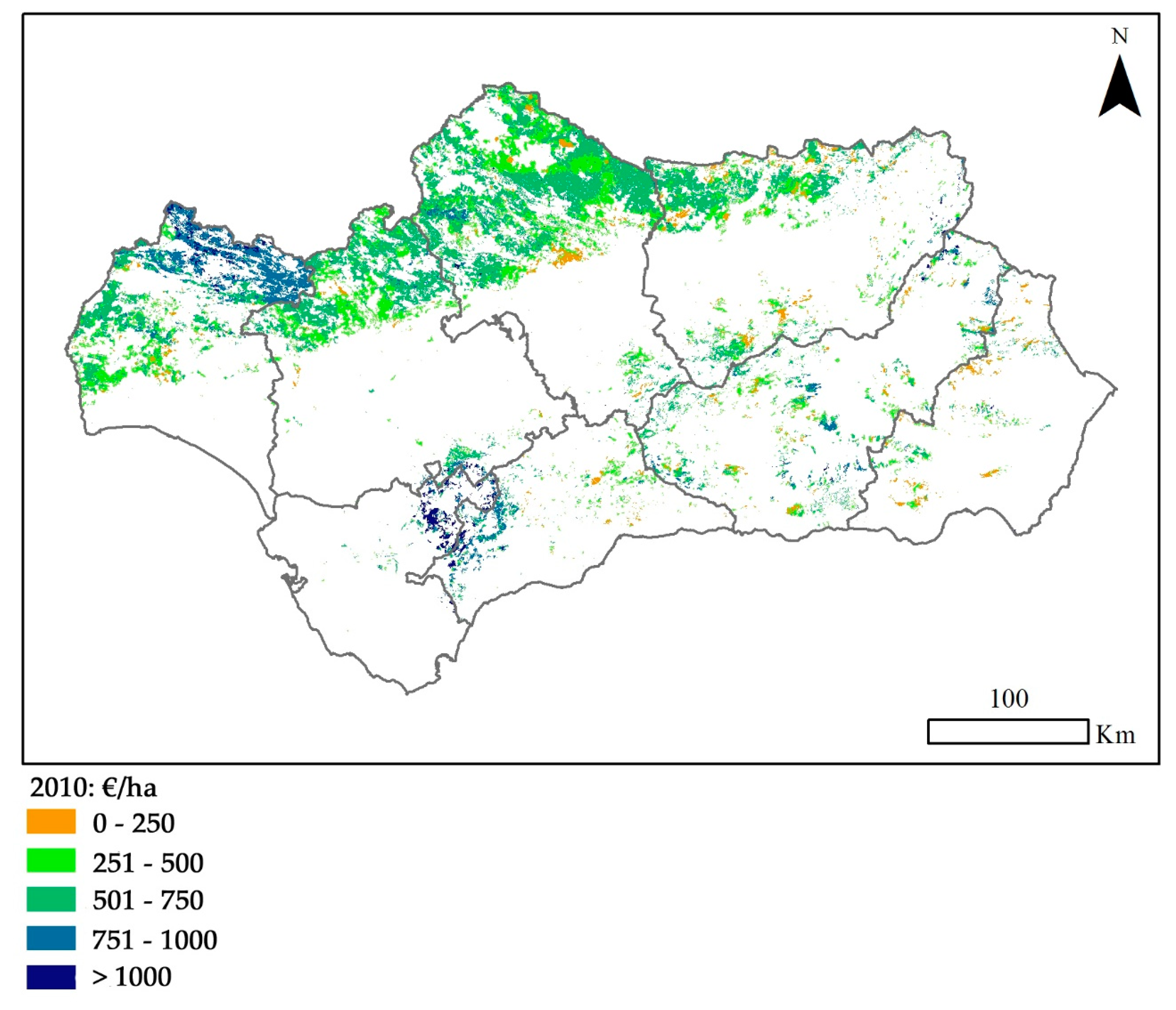
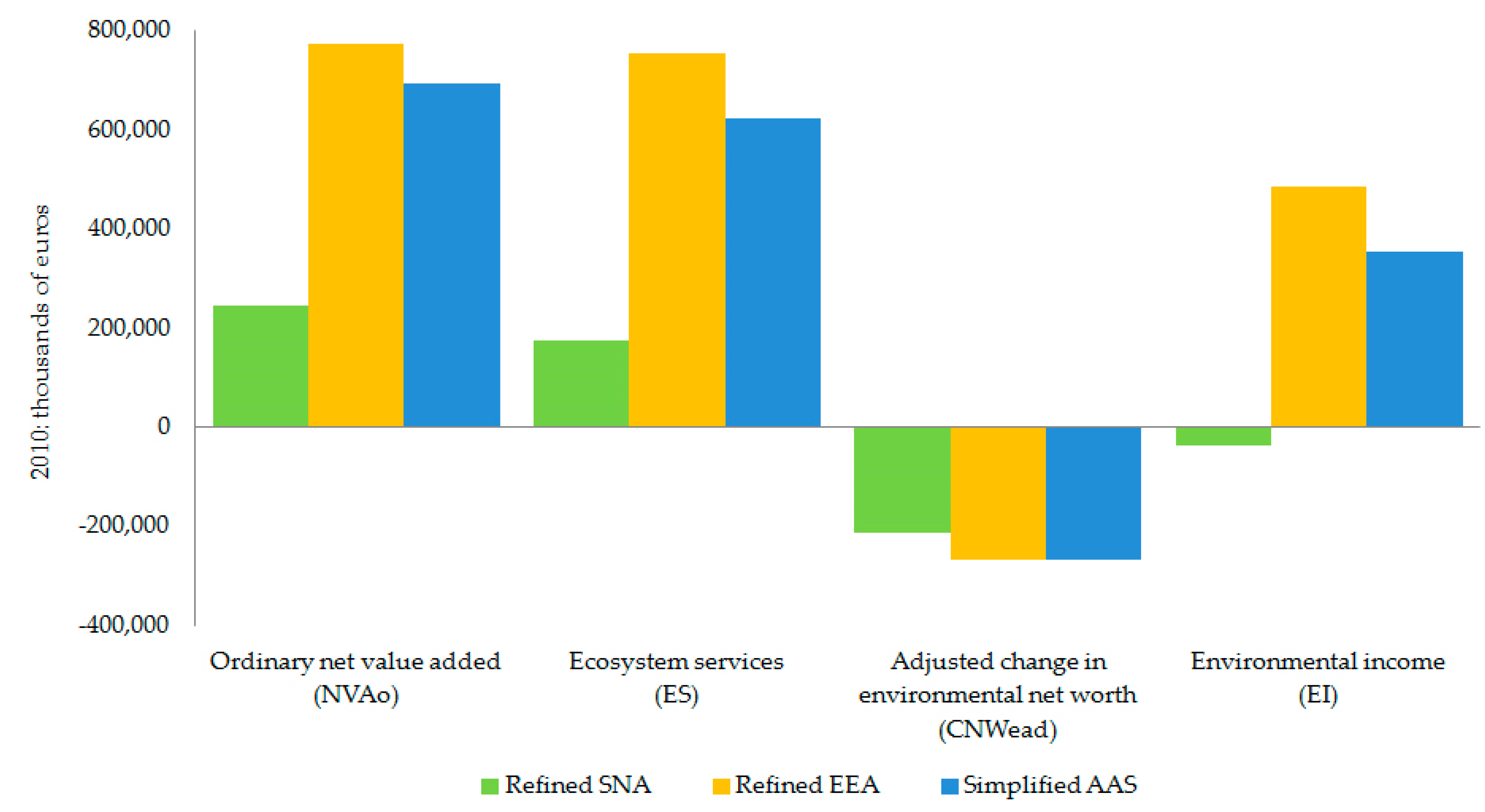
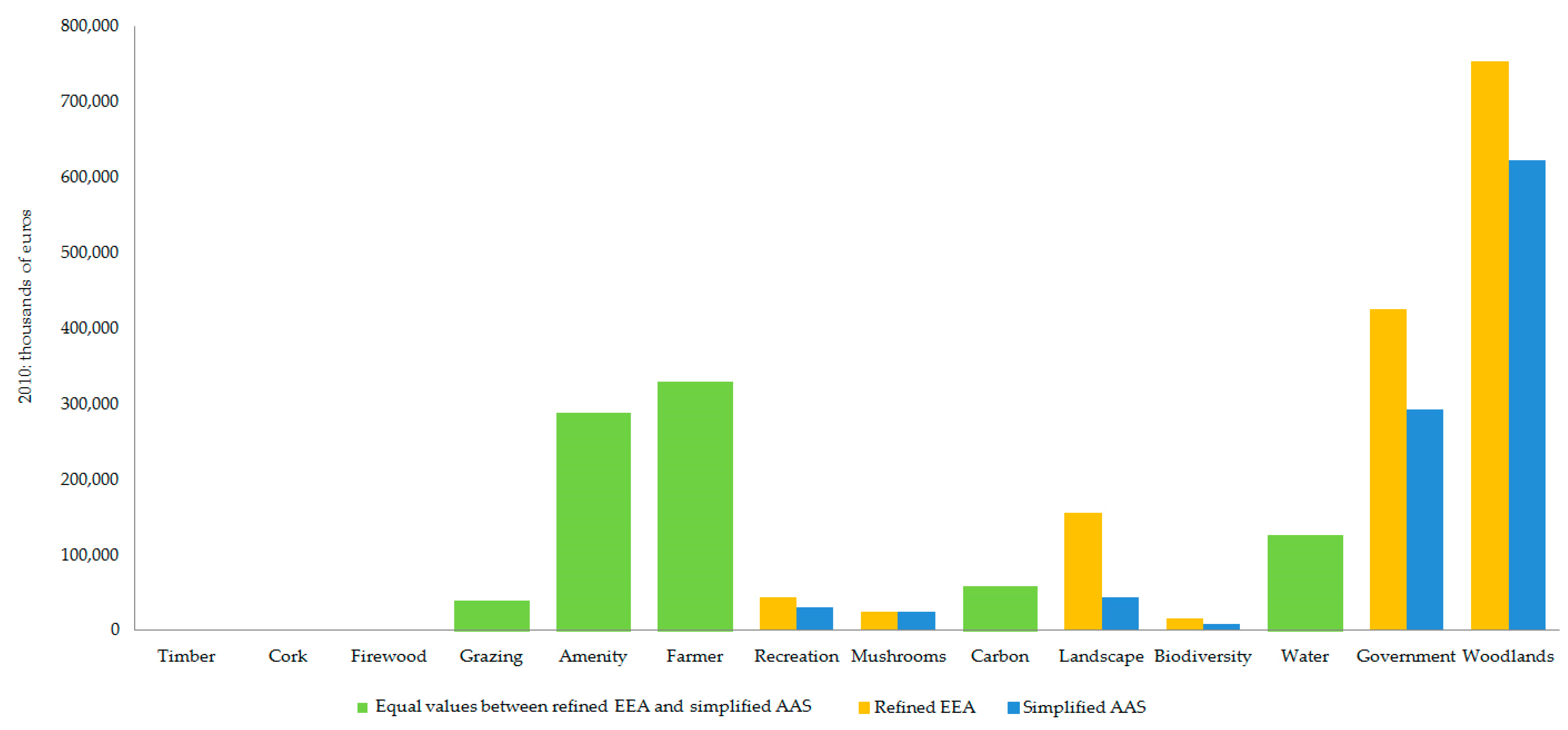


