Retrieval of Forest Structural Parameters from Terrestrial Laser Scanning: A Romanian Case Study

Abstract

Research Highlights: The present study case investigates the differences occurring when tree’s biophysical parameters are extracted through single and multiple scans. Scan sessions covered mountainous and hill regions of the Carpathian forests. Background and Objectives: We focused on analyzing stems, as a function of diameter at breast height (DBH) and the total height (H), at sample plot level for natural forests, with the purpose of assessing the potential for transitioning available methodology to field work in Romania. Materials and Methods: We performed single and multiple scans using a FARO Focus 3D X130 phase shift terrestrial laser scanner at 122 kpts and 0.3:0.15 mm noise compression ratio, resulting in an average point density of 6pts at 10m. The point cloud we obtained underpinned the DBH and heights analysis. In order to reach values similar to those measured in the field, we used both the original and the segmented point clouds, postprocessed in subsamples of different radii. Results: Pearson’s correlation coefficient above 0.8 for diameters showed high correlation with the field measurements. Diameter averages displayed differences within tolerances (0.02 m) for 10 out of 12 plots. Height analysis led to poorer results. For both acquisition methods, the values of the correlation coefficient peaked at 0.6. The initial hypothesis that trees positioned at a distance equivalent to their height can be measured more precise, was not valid; no increase in correlation strength was visible for either heights or diameters as the distance from scanner varied (r = 0.52). Conclusions: With regard to tree biophysical parameters extraction, the acquisition method has no major influence upon visible trees. We emphasize the term “visible”, as an increase in the number of acquisitions led to an increased number of detected trees (16% in old stands and 29% in young stands).

1. Introduction

Forest inventories are the main way of deriving information on forest stand characteristics for a range of fields including biometrics, forest monitoring, physiology and for appraising forest biodiversity or the success of forest management practices. Over the last decade, technological advances in terrestrial laser scanning (TLS) have allowed the development of highly portable, accurate and increasingly cost-effective sensors. Similarly, we can observe an increase in data processing solutions capable of segmenting and reconstructing accurate individual tree models [1,2,3]. This facilitated the use of such close range remote sensing technologies for describing forest stands structural parameters [4,5,6] and biophysical parameters [7,8,9].

TLS techniques facilitate virtual revisiting of the same forest stand once it has been scanned. This allows analyzing and testing hypotheses beyond those which initially led to the acquisition of the data. In addition, research and knowledge on TLS processing in forest ecosystems can be applied to predating sets of data [10]. Multiple scans processing [11,12], and several TLS scanning distances [7], have previously been used to assess the quality of tree parameter extraction, sometimes even using a species-specific approach [13]. Most of the studies on the extraction of forest biophysical parameters from TLS data focused either on plantations or on small areas of natural growth forest, and analyzed various size plots (from sample plot to forest stand level) [14,15].

The aim of our study is to assess the potential of transitioning the theoretical methodologies (e.g., point cloud classification, segmentation, voxelization, 3D reconstruction) towards a forest inventory oriented tool, specific for the Romanian forest monitoring activities. What was previously used for single tree scanning (as a means of analyzing the forest ecosystem in a controlled environment) needs to be transferred to full-scale fieldwork by overcoming the construction limitation of the TLS (narrow field of view) in the most productive manner. Besides the limitations of the technology itself, there is also a reluctance towards assimilating such close-range ground-based remote sensing approaches in Romanian forestry, that should be taken into account. In order to reach our aim, and asses the level to which the expert knowledge in terrestrial laser scanning can be passed to personnel from other areas, we had to restrict the acquisition, processing and interpretation of the data to preexistent algorithms and software. This is a major factor in the acceptance of the research as a tool in areas that might benefit from it.

Multiple studies have focused on the detection of biophysical parameters at both stand and individual scale, with major findings. Heinzel and Huber [16] reached close to 100% identification of stems position by focusing on close range segmentation; similar results are reiterated in several other papers [14,17]. With similarly good results, studies on biophysical parameters estimation covered both diameter [18,19,20] and heights evaluation [21,22]. There are still some factors that constrain the applicability of the technology, leading to the impossibility of gaining such results for all interest aspects (e.g., diameter, height, volume, crown area). But even so, research covering the aspect of combining point clouds from multiple positions [23] or that of pre-designing the acquisition network [24] as compensating measures. As such, for most of the intended goals, we followed and extended the previous work addressing both tree and stand level [25,26], forest type influence [27] and even terrestrial laser best practice guides [28,29].

We investigated and quantified the differences that occur when reconstructing trees at sample plot level from single scan versus multiple scans in deciduous and coniferous dominated forests. We also analyzed the influence of the distance variance between the scanner and the furthest targeted stem in both single and multiple scans. As a result, our case study serves as a good practice guide with focus on Romanian forest ecosystems, by addressing the subject at country specific reach level. By evaluating the degree to which the above-mentioned results and approaches can be reached through pre-existing software [30,31,32,33,34,35,36,37] and mid-range field equipment [35], we can facilitate the acceptance of terrestrial laser scanning as a tool in Romanian forestry. The current study case needs to answer the following questions: can available tree reconstruction methods be applied at a larger scale in natural forest stands, by non TLS-centric users? What are the limitations of single and multiple scanning approaches when increasing the study area– can this limit in any way the extent to which the technology can be used in the field? Is the extra effort implied by multiple scans reconstruction translated in an increase in quality or quantity of the results?

2. Materials and Methods

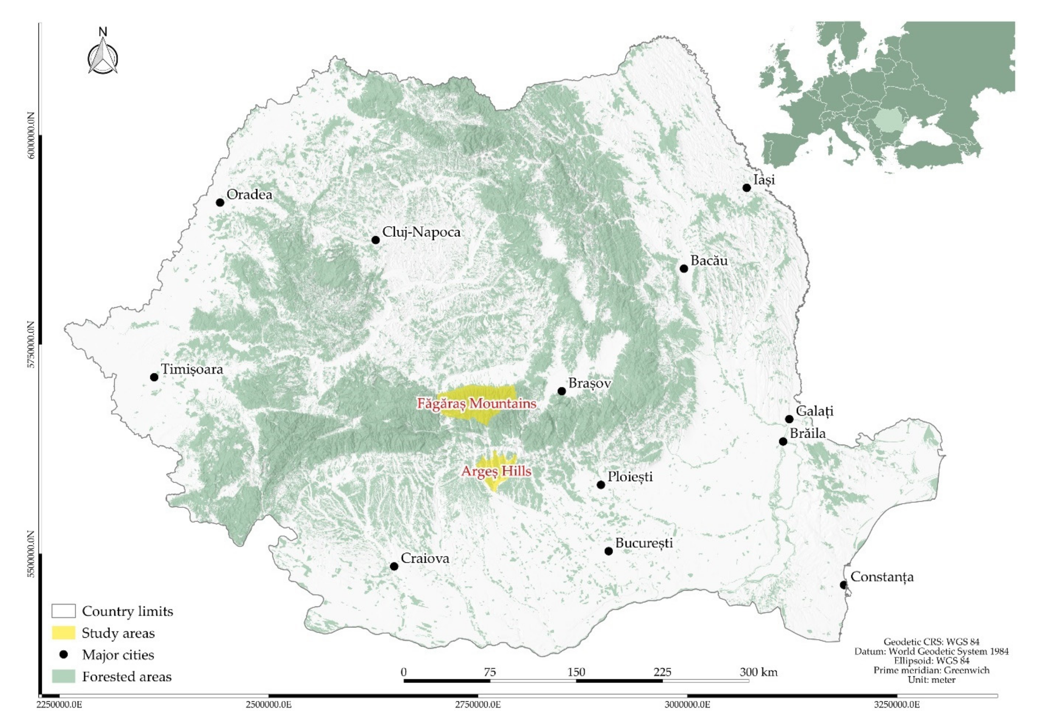
2.1. Study Area

We have conducted field inventory activities in twelve circular plots with a radius of 15 m each, grouped in two sets. The plots were set in the mountainous and Subcarpathian hills’ forests in central and southern Romania (

Table 1. Forest stand characteristics of the sample plots included in the case study.

Forest District	Location [WGS84]	DBH.m. [cm]1	No. Replicates2	Stdev3	H.m. [m]4	No. Replicates5	Stdev3	Species	Age [years]	Ρ6
Mihăești	45°06′32.6”N 25°00′42.9”E	10	2	3.4	13	3	2.6	SoY7	50	1
		52	2	16.1	26	3	8.7	SoO8	190	1
Mușătești	45°25′19.7”N 24°41′14.4”E	22	2	9.1	20	3	6.2	SY9	50	1
		40	2	12.6	27	3	6.8	SO10	150	1

¹ Mean diameter at breast height; ² Orthogonal measurements;³ Standard deviation; ⁴ Mean height; ⁵ Measurements along the isoline from distances equal to the height of the tree; ⁶ Ratio between canopy area without crowns overlap and plot area; ⁷ Sessile oak young (Quercus petraea); ⁸ Sessile oak old (Quercus petraea); ⁹ Spruce young (Picea abies); ¹⁰ Spruce old (Picea abies).

). The plots were selected by taking into consideration the species and age class (O-old, Y-young), namely sessile oak (So), Quercus petraea (SoO 1, 2, 3; SoY 1, 2, 3) in the hill region and norway spruce (S), Picea abies (SO 1, 2, 3; SY 1, 2, 3) in the highlands (Figure 1). We selected the species for their representativeness within the Romanian forest ecosystem, allowing for the assessment of the studied methods in both deciduous and coniferous plots of various structures.

2.2. Field Data Collection

2.2.1. Reference Measurements

We focused reference field measurements on recording diameter at breast height (DBH), height (H) and position of each tree (XYZ). The DBH values were computed as an average between two caliper measurements taken at right-angles and for the heights a digital hypsometer was used. In order to determine the position of each tree, FieldMap [38] (Integrated GIS field software coupled with electronic mapping and dendrometrics sensors) measurements were carried out. These measurements will underpin the validation of TLS processing results.

2.2.2. Single terrestrial laser scan

We performed a single terrestrial laser scan from the center of each plot with a FARO Focus 3D X130 phase shift terrestrial laser scanner at the same time with the above-mentioned field measurements. Allowing 8 µs per scan point for each of the 44.4 million samples of the scan, increased the signal strength in recording reflectance values. We considered the scan origin as the central position, as this was also used as a reference in the field measurements.

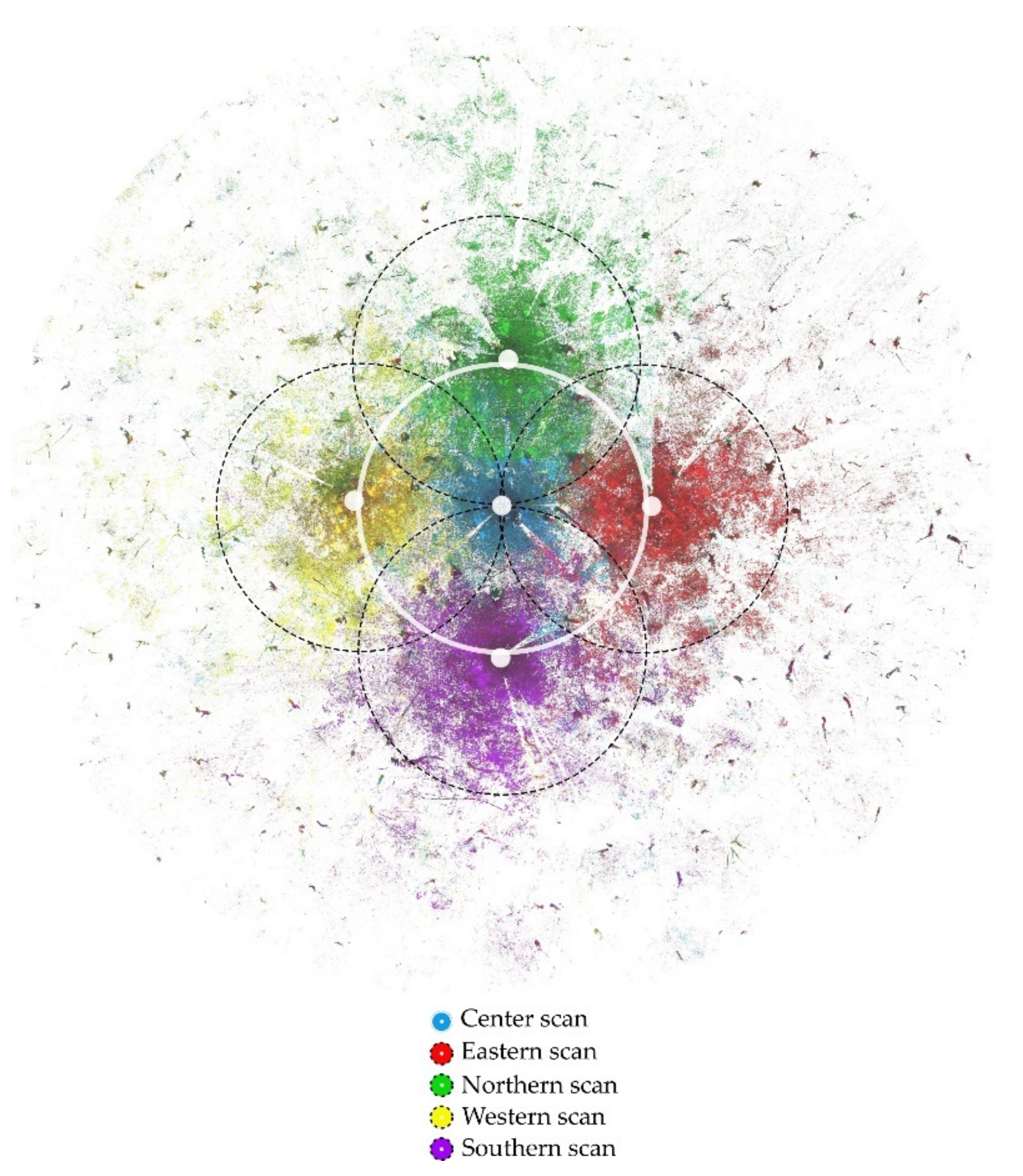
2.2.3. Multiple Terrestrial Laser Scans

The multiple TLS approach aimed at increasing the number of points whilst simultaneously standardizing their density through a five-scan composition. This was done to estimate whether the difference in acquisition method translates to an increase in the number of identified trees and furthermore in the sample plot reconstruction accuracy. Also, by scanning the same plot from several directions, shadow cones were mostly eliminated.

Forest inventory procedures regarding height measurement require a viewing distance equivalent to the height of each tree projected along the local terrain contour. Based on this and the general aim of running the analysis at the plot level, the position of each scan was set at the 15 meters mark. This reduced the risk of missing any of the peripheric stems. We ran four scans from radial positions, alongside a central scan. To compare the results from different plots, we established a repeatable methodology - to position the scans on the directions of the compass points (Figure 2).

Seven spheres (0.07 m radius) were used as coregistration markers, as their shape suffers no warp with the change of the scan perspective [39]. The positioning at variable heights raised them above the understory vegetation. Their increased visibility translated to increased coregistration confidence. Each sphere was placed so it could be recorded from the central scan and from at least two more stations.

Previous to starting any of the scans, we set all stations to ensure maximum visibility. This required superficial pruning, especially in young spruce sample plots, increasing the time allocated to one scan from ~8 min to almost 30 min.

2.3. Terrestrial Laser Scans Pre-Processing

Prior to the reconstruction stage, the raw scans were coregistered. We connected individual scans using a semi-supervised target-based approach, using the spheres as references, followed by a cloud to cloud control stage [35]. This extra level of control implied refining of the rough positioning by semi-supervised sphere identification, based on onboard inclinometer and compass data. The cloud to cloud optimization was done on a cropped, evenly sub-sampled point cloud (0.08 m density threshold). Coregistration precision values were within tolerances (0.02 m/pair of scans–strong coregistration; 0.02–0.04 meters–medium-strength coregistration; >0.04 meters–weak coregistration) [35], averaging between 0.004 and 0.018 m. Any error exceeding the accepted tolerance for biophysical parameters (0.02 m) required supervised coregistration (

Table 2. Error values in the case of multiple scans processing.

ID	Min.Con.1	Max.D. Error [m]2	Max.Hz. Error [m]3	Max.V. Error [m]4
SoY 15	4	0.0073	0.0071	0.0039
SoY 25	4	0.0078	0.0077	0.0055
SoY 35	4	0.0072	0.0071	0.0016
SoO 16	4	0.0184	0.0175	0.0058
SoO 25	4	0.0082	0.0080	0.0030
SoO 35	4	0.0101	0.0100	0.0040
SY 17	4	0.0069	0.0069	0.0058
SY 27	4	0.0136	0.0075	0.0113
SY 37	4	0.0068	0.0067	0.0030
SO 18	4	0.0051	0.0051	0.0038
SO 28	4	0.0053	0.0037	0.0052
SO 38	4	0.0038	0.0031	0.0023
mean	4	0.0084	0.0075	0.0046

¹ Minimum number of connections for each scan; ² Maximum error for distances computed two ways; ³ Maximum error for horizontally normalized distances; ⁴ Maximum error for vertically normalized distances; ⁵ Young sessile oak stands; ⁶ Old sessile oak stands; ⁷ Young spruce stands; ⁸ Old spruce stands.

).

After exporting the coregistered data as a coherent point cloud, the ground defining points were separated. This simplified subsequent processes by concentrating only on the vegetation. The process was an iterative one, with a three-dimensional (3D) window of 0.2 m height and a footprint of 0.8 square meters. A threshold of 128 points per grid cell (for the selected grid size) was chosen [40]. Noise was removed from the ground cloud by analyzing the normal orientation of each point, based on six nearest neighbors. The filtered cloud was then interpolated to generate a digital terrain model (DTM) of 0.1 m resolution.

The last step before reconstruction was cloud segmentation or classification of the point cloud into clusters that define individual trees. To facilitate the segmentation stage, several cleanup procedures have been undertaken. A simple way to bypass the understory vegetation, and the low-lying branches was to create a section of defined height (0.3 m) at a constant elevation above the DTM (2 m). This spatial sub-sample aimed to simplify the stem identification stage. Noise was removed from the resulting slice using the before mentioned method by changing the reference surface from a theoretically horizontal ground to a surface closer to vertical for the trunks. A fast spatial clustering based on the work of Hackenberg et al. [7] was applied to segment trunk seeds. We defined a seed as any cluster of points containing at least 0.1% of the total point cloud, but not less than 400 points. We separated the output into two classes through Euclidean clustering, based on the distance between points (0.10 m threshold). Out of the two resulting classes, one was characterized by a lower number of clusters with a higher percentage of representation in the original point cloud, whilst the other had a significantly higher number of clusters, with a reduced percentage of the total. Starting with these seeds, the clusters were expanded in the original vegetation point cloud in a vertical direction. Slices were generated at 0.10 m intervals and the same Euclidean clustering was applied. Instead of expanding the clusters based solely on the distance between points, the distance to the previous seed was also taken into consideration. A cylinder was fitted to each newly created cluster. If the projected center of the fitted cylinder fell inside the original seed footprint and its specific radius was a solution of Equation (1) (n = 1.2–as an average of the minimum/maximum values provided by Bitterlich, 1978), then the cylinder was considered as being part of the same tree. Clusters with less than 10 points or with a radius exceeding the tolerances were dropped and merged in a residual point cloud to be reprocessed in the following repetitions. The iteration continued until it reached the end, by either hitting the lowest Z value or by not generating any clusters that met the conditions above.

$${\mathrm{r}}_{\mathrm{h}}=\frac{{\mathrm{x}}^{\frac{1}{2}}\times {\mathrm{h}}^{\frac{\mathrm{n}}{2}}}{2}$$

(1)

h—height

r_h—radius at height h

n—geometry type coefficient

x—surface of revolution generator

Equation (1) resulted from the initial assumption that a tree trunk can be reduced to a 3D primitive (the simplest geometric object that can represent the stems). But the structure of a stem, with a concave base and a slight convex middle accentuated towards the top, better resembles a neiloid. By not considering this taper, cylindrical representations would generate unrealistically large volumes and tolerances; a paraboloid would be the next best geometry to represent the volume of a stem, with cones midway between the tapered shapes. Neiloids would yield the least excess-volume of all the considered shapes (Figure 3). A theoretical n value would vary between 0 for a cylinder and 3 for a neiloid. However, these values do not lead to realistic results. The literature recommends an n value between 0.9 and 1.5 to best define the real shape of a stem [41].

Two filters have been applied, addressing spatial extent and density. In the first case, clusters with a height of below 3 m or above 60 m have been removed. For point density, clusters with less than 15,000 points, were removed. Both processes were performed using CloudCompare (scalar fields - compute stat. param) [30] and Quantum GIS tools (vector geometry - bounding boxes) [37].

Down-sampling of the voxel grid reduced the size of the resulting clusters to facilitate the extraction of biophysical parameters. To limit the information loss, for each 3D cell or voxel (0.01m) the centroid of the contained points was extracted and used, rather than the centroid of the voxel itself. The mean distance to the nearest points was computed and based on the condition in Equation (2), some points were excluded. The voxel grid was implemented to reduce the processing power needed for the subsequent stages by using lidR and lasvoxelize packages for R [36,42]. This step implied reducing the number of points through the intersection of the point cloud with a 3D grid of the same extent.

$$\left|\overline{\mathrm{d}}-\mathrm{x}\times \mathsf{\sigma }\right|< \overline{\mathrm{d}},$$

(2)

$\overline{\mathrm{d}}$—mean distance

$\mathsf{\sigma }$—standard deviation

x—threshold for angle between neighboring normals

Previous research showed that $\overline{\mathrm{d}}\pm \mathsf{\sigma }$ (x = 1) is enough to identify outliers [43].

2.4. Terrestrial Laser Scans Processing

With the original point cloud cleaned and segmented, diameters and heights could be extracted. Besides these two parameters, the position of each stem had to be recorded in the same reference system as the field data to identify the correspondences between them.

Each stem position was computed as the average point location (X, Y) within a 0.1 m tall cylinder. The altimetric position was computed as a mean valueof the points lying inside a best-fitting cylinder above the ground, with a height of 0.1 m.

The DBH was determined by extracting a section parallel to the DTM, between 1.25 and 1.35 m and identifying the true stem (no branches) through a randomized Hough transform (weight based analysis for detecting shapes in 3D point clouds) [44]. Afterward, a circle was fitted using the least square regression. The height, or vertical projection of the stem, was computed in two ways, as TLS based height estimation usually leads to erroneous results. This way, two sets of height values were obtained, allowing for further evaluation of their accuracy against field measurement. The first approach was based on computing the maximum difference on the Z-axis between its DTM elevation and the top of the vegetation cluster. In the second approach, the height was computed as the highest Z value enclosed inside a cylinder of diameter equal to the stem’s DBH, from the unfiltered cloud. In the case of trees with an obvious lean (either recorded during field observations or identified during any of the supervised processing stages), the length was used instead of the height. The length was computed as the maximum distance between any two points in the tree cluster.

3. Results

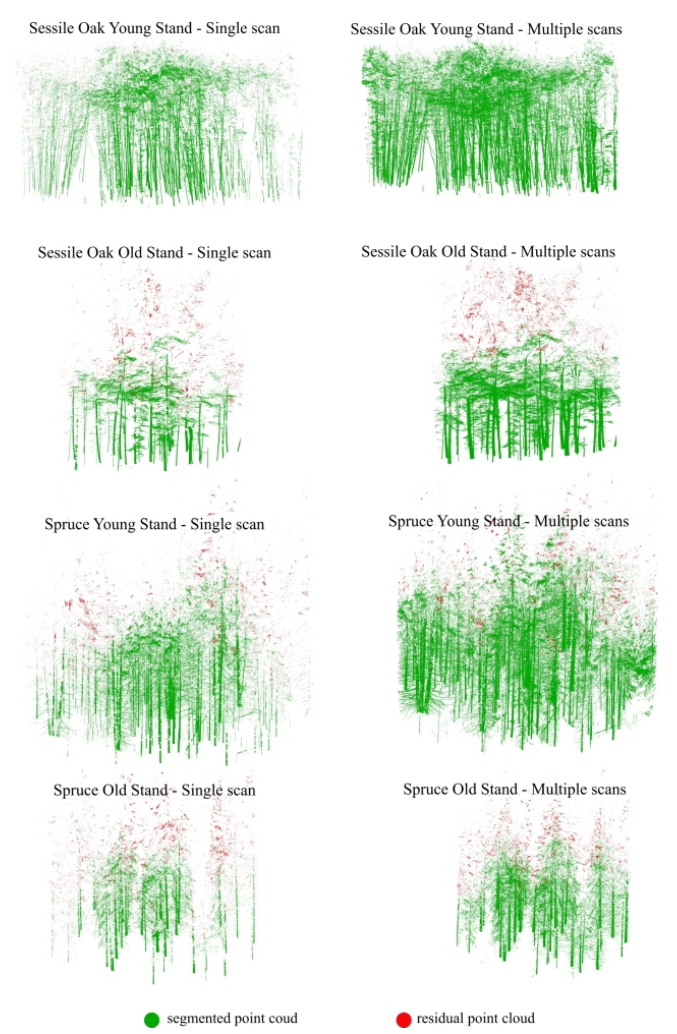
3.1. Individual Tree Segmentation

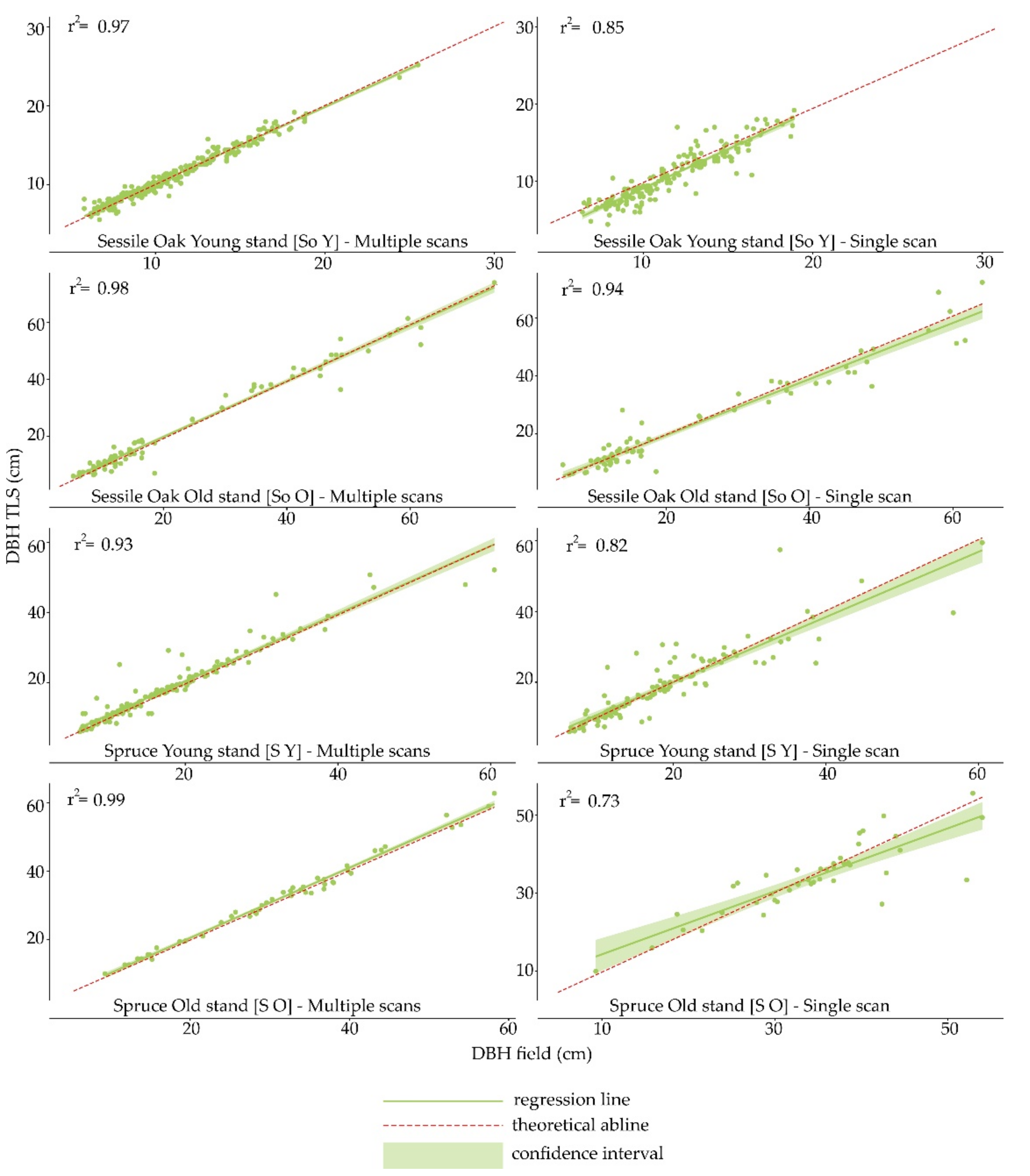
The precision of TLS reconstruction was evaluated based on the accuracy of the diameters, heights, and number of extracted individuals for the two scanning approaches. To assess whether or not multiple scans led to more accurate results, individual trees have been identified and mapped in both the TLS point clouds (single and coregistered multiple) and in-field measurements. One to one join was used to allow comparing them as identical data sets and assess only the quality of the extracted biophysical parameters (DBH and height). Consequently, both the field and the multiple scan data sets were subsampled to only display those individuals identified through single scanning since it provided the lowest number of stems (

Table 3. Differences regarding the number of identified trees between single and multiple scans.

ID	S.1	M.2	F.M.3	%M.4	%S.5	%Inc.6
SoO 1	26	31	36	86	72	13.89
SoO 2	25	34	45	76	56	20.00
SoO 3	21	31	48	65	44	20.83
SO 1	17	20	31	65	55	09.68
SO 2	10	15	28	54	36	17.86
SO 3	12	14	20	70	60	10.00
SoY 1	63	110	135	81	47	34.81
SoY 2	47	95	130	73	36	36.92
SoY 3	65	93	114	82	57	24.56
SY 1	46	60	92	65	50	15.22
SY 2	41	74	106	70	39	31.13
SY 3	30	30	87	34	34	00.00

¹ Number of trees from single scan; ² Number of trees from multiple scans; ³ Number of trees from field measurements; ⁴ Percentage of extraction from multiple scans in relation to field measurements; ⁵ Percentage of extraction from single scan in relation to field measurements; ⁶ Percentage of increase/decrease between multiple and single scans.

).

The increase in the number of identified individuals is substantial when switching from a single central scan to a coregistered point cloud. Also, a relationship between the sample plot’s structure (age and species) and segmentation quality was observed, as the number of detected trees increased by 16% for multiple scans in old sample plots and by 29% in young sample plots. By species, multiple scans detected on average 25% more trees when compared to single scans for sessile oak and only 18% more for norway spruce sample plots.

3.2. DBH Estimation

When analyzing the quality of extraction (diameter and height), the positive influence that the increased point cloud density had on stem extraction was not replicated in the biophysical parameters’ evaluation.

A comparison between the trends of the diameter values in relation to a theoretical abline (constrained by a constant relation between the two data sets) was carried out to better differentiate the two scanning approaches. Single scans displayed an overall underestimation of large diameters, regardless of the species or age of the plots (deviation within 0.3–3.6 cm). Moreover, in old sample plots, the underestimation of large DBH values was coupled with an overestimation of smaller DBH values. This effect is reduced when processing multiple scans. Regarding the overestimation of young trees’ DBH and underestimation of old trees’ DBH, the phenomenon can be explained by the natural evolution of trees. Young trees tend to maintain a more cylindrical stem shape, whereas old trees, because of different stress and environmental factors, develop in a more irregulate manner. This process is called ovalization (Figure 4).

In the case of multiple scans, inconsistencies occurred only in spruce sample plots where old plots did not just maintain an overestimation for small DBH, but also extended the effect slightly towards the larger values.

In contrast with the visible DBH underestimation in the single scan results, multiple scans overestimated DBH values in spruce sample plots. It is worth mentioning here, that spruce plots are characterized by an uneven DBH distribution. Only when overlooking the spruce sample plots, can multiple scans approach be considered to have a regulating effect on diameter values, eliminating over- or under-estimation tendencies (

Table 4. Evaluation of extracted DBH in relation to real values.

ID	S.1	M.2	F.M.3	ΔFM-S4	ΔFM-M5
SoO 1	26.9	26.0	25.6	−1.3	−0.4
SoO 2	19.4	19.9	19.4	0.0	−0.5
SoO 3	10.9	20.1	20.0	9.1	−0.1
SO 1	34.2	31.5	30.8	−3.4	−0.7
SO 2	30.6	32.7	32	1.4	−0.7
SO 3	35.6	32.5	31.5	−4.1	−1.0
SoY 1	10.7	11.3	11.1	0.4	−0.2
SoY 2	10.4	10.5	10.4	0.0	−0.1
SoY 3	11.1	11.7	11.6	0.5	−0.1
SY 1	16.8	17.4	16.4	−0.4	−1.0
SY 2	17.5	16.7	16.5	−1.0	−0.2
SY 3	22.9	21.1	20.8	−2.1	−0.3

¹ Mean DBH from single scan; ² Mean DBH from multiple scans; ³ Mean DBH from field measurements; ⁴ Difference between field DBH and single scan DBH; ⁵ Difference between field DBH and multiple scans DBH;.

). Despite the slight under and over-estimation, the diameter values strongly correlated to the field measurements (Figure 5), with r values reaching above 0.9. This relation was reflected in the strength of the determination coefficient, r² which averaged a value above 0.9. Despite the largely similar results, important differences were observed at some sites between single and multiple scans. For example, for SO 1 the r² coefficient (with respect to the field measurements) changed from 0.33 to 0.98 from single to multiple scans.

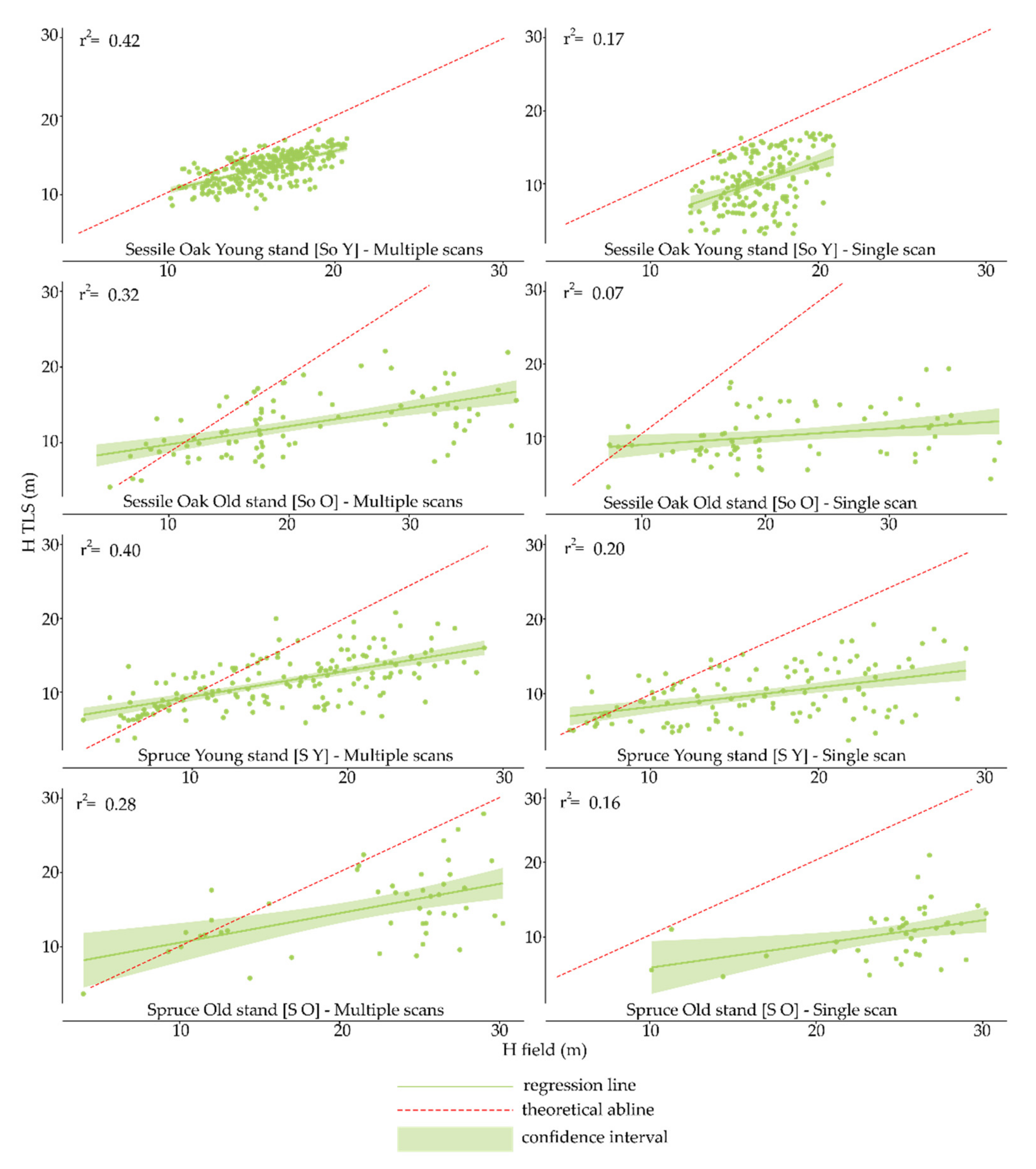
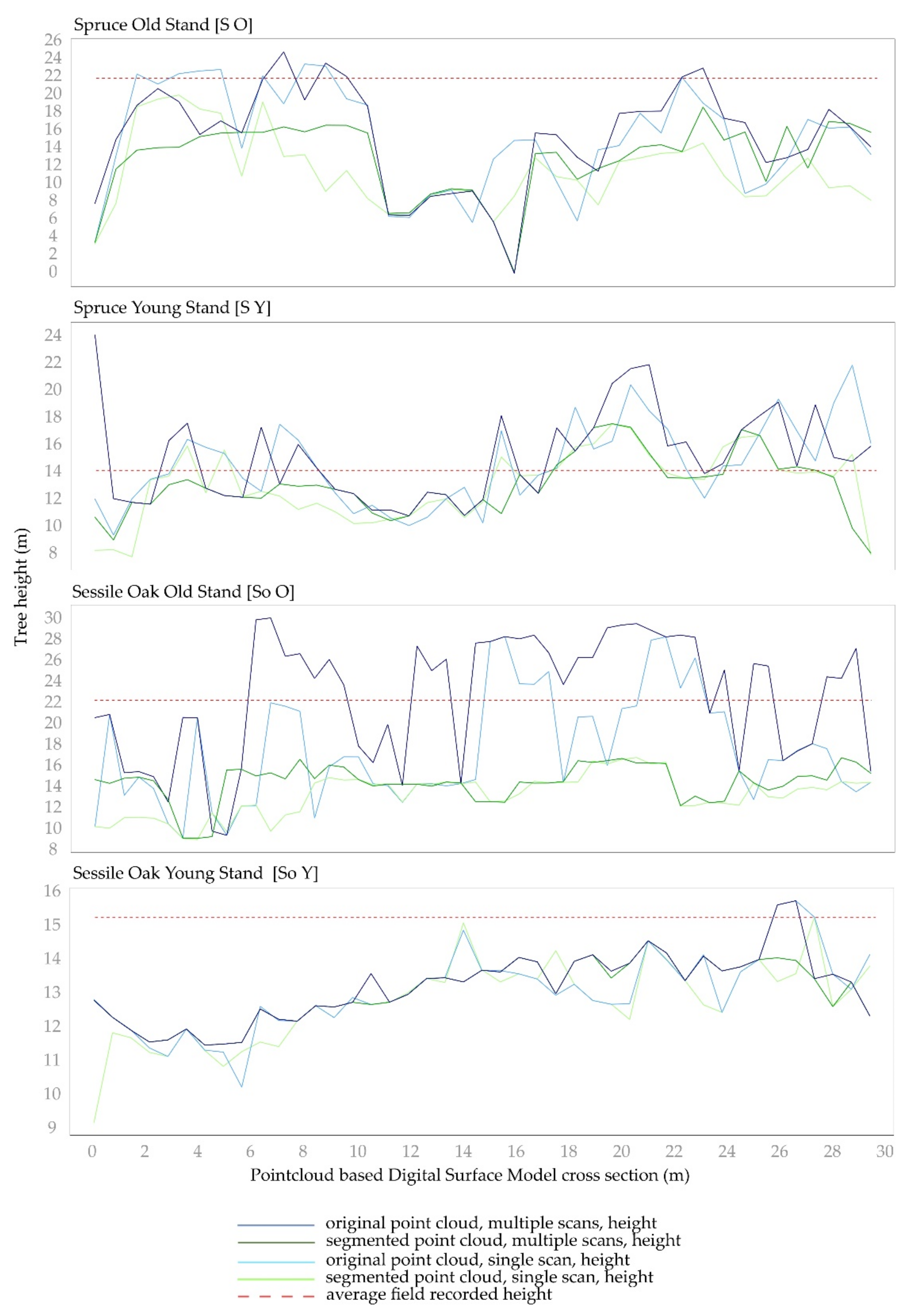
3.3. Height Estimation

Significantly weaker correlations (Figure 6) were reached in the case of heights estimation (r < 0.76) with determination coefficients of up to 0.59. Switching from single to multiple scans slightly improved the results from r² of 0.31 for single scans to r² of 0.41 for multiple scans.

Another analysis was conducted to examine whether the distance to the scanner impacts the results. The hypothesis was that trees at a distance equivalent to their height can be measured more precisely [45]. In the same acceptance, the closer one gets to the scanner, the better the diameter can be represented and measured. To evaluate this supposition, the plot radius of 15 m was divided into two segments upon which spatial filters have been applied. The filtering consisted in the creation of a buffer around the centre of the plot with a radius of 7 m and its intersection with the position of the trees. The results showed no increase in correlation strength for either heights or diameters, as the distance from scanner increased (r = 0.52 for the entire plot vs. r = 0.62 closer than 7 m and r = 0.59 further than 7 m). Regarding diameters, there is no difference reflected in the correlation coefficients (r for the entire plot equals that of values subsampled closer than 7 m and that of values sampled further than 7 m, 0.94).

By comparing the results of the two methods used for the estimation of height, the quality of the segmentation and tree reconstruction could be assessed. The old sample plots were characterized by a bigger residual cloud, whilst reconstruction based on young sample plots point clouds resulted in sparse residual clouds (represented in Figure 7 as the area between the Digital Surface Models (DSM) based on the original and the segmented point clouds).

As seen from

Table 5. Descriptive statistic on heights extracted before and after segmentation in relation to field values.

		Mean [m]	Min. [m]	Max. [m]	St.Dev.	ΔMean [m]	ΔMin. [m]	ΔMax. [m]
	segmented	13.3	8.6	17.6	1.3	1.9	1.7	2.7
SoY 1	original	13.6	10.1	17.6	1.3	1.6	0.2	2.7
	field	15.2	10.3	20.3	1.8
	segmented	15.3	8.3	20.6	2.2	7.1	−1.5	18.2
SoO 1	original	23.0	8.4	32.3	5.9	−0.6	−1.6	6.6
	field	22.4	6.8	38.9	10.4
	segmented	11.4	3.4	18.4	2.6	2.9	1.9	10.4
SY 1	original	13.9	3.4	26.6	3.9	0.4	1.9	2.2
	field	14.3	5.3	28.8	6.2
	segmented	13	3.0	20.2	3.6	9.0	6.3	9.3
SO 1	original	17.3	4.6	29.8	5.3	4.7	4.7	−0.3
	field	22	9.3	29.5	6.5

, no matter the age, the heights are underestimated (mean underestimation for old sample plots reaches 37% (± 25%) and for young sample plots 14% (± 19%) of the mean real height of the plot) in the sessile oak study area. For spruce areas the mean underestimation is even greater, reaching values of 35% (± 31%) for young trees and 44% (± 27%) for old trees. Both height estimation techniques (segmenting and maximum height per crown projection) lead to unsatisfactory results, suggesting that single wavelength TLS in leaf-on conditions is not suitable for extracting height values at the plot level, because of difficulties in penetrating dense canopies (Figure 8).

4. Discussion

The current study case may not have provided significant improvements in the extraction accuracy for the biophysical parameter, but can be used as a guideline. Comparison and contrast-based optimization using a mid-class terrestrial laser scanner in natural growth forests, covered the gap between controlled research and field implementation. Results are therefore similar to some degree to that of previous research, although our approach focused on sample plot level in natural forests.

When analyzing diameter extraction, we found multiple scans approach to lead to an increase in precision. This does not invalidate single scan results, as the differences are within measuring tolerances. Despite this, a significant improvement arising from multiple scans approach is the number of identified trees, which in terms translates into a more accurate stand level estimation of all the biophysical parameters. The use of multiple scans in DBH evaluation would be beneficial for transitioning from circular fitting to an ellipse. Having a more accurate representation of the stem (as the one resulting from the multiple scans) could yield better values for the semi-major and semi-minor axis of the ellipse. Since none of the height extraction methods could provide realistic estimations, investing time in multiple scans approach is not recommended. The shadowing and occlusion effects could not be fully compensated by multiple scanning. A potential solution could be the use of a dual-wavelength full-waveform terrestrial laser scanner [46]. The stand structure (density, species, age) and local topography had an influence upon the height’s estimation, but different conditions would have not differentiated between the used methods.

Since the method for estimating DBH is based on the least square error when best fitting a circle, straying away from the circular shape increases the error of radius estimation. A solution might be found in increasing the number of iterations involved in extracting DBH values, but better still would be moving to a two dimensional (2D) ellipse fitting [47]. Even so, the DBH values that we obtain were similar to those highlighted in recent papers (average RMSE of 3 cm) [25,48,49].

The low values observed for the correlation coefficients between heights extracted from FieldMap [38] and TLS did not improve when the number of scans increased. An increase in the number of scans proves to not increase the strength of penetration of the canopy. As a result, tree tops are still not reachable.

In an intra-species comparison, when analyzing the influence of the sample plots’ age, the residual point cloud displays a rise in both density and coverage with the increase in age. This translates into a decrease of the vertical reach as age increases. Age variation generates a more complex structure, and with higher diameters and densities (above a threshold of 0.5 m/0.7 consistency-see Table 1), we expect lower relative height values.

The increase in the proportion of identified stems between single and multiple scans (10%) observed by Xi et al. [15] was confirmed but with higher values (16 to 29%). Literature provide overall detection percentages to exceed 97% [16,17], with a slight decrease for smaller diameters. Although depended on the structure and number of scans [24], the ~10% decrease is similar to our results. Height estimation remained an issue no matter the species or sample plot structure, similar to Saarinen et al. [11]. The slight precision increase in close range scans, also mentioned in previously published papers [45], was considered of no significant value. This conclusion is supported by the Wilcoxon signed rank test which results in p-values smaller than of 1×e⁻⁵ for both close (7m radius) and far (15m radius) range. Computing the cosine similarity of both close and far range height trends to the normal, once again confirmed their similitude (average value of 1.5×e⁻³ ± 2×e⁻³). Different conditions led to improved values in Height evaluation in similar research (average RMSE of 7 cm [50,51]).

If the aim is to identify the number of individuals, multiple scans technique is the proper way to acquire data. As very few investigations require solely the number of individuals and their positions, this might not represent an advantage of multiple scans over single scans.

5. Conclusions

TLS proved to be a suitable solution in some aspects of forest monitoring and inventory activities. The wide range of applications confirms TLS’s utility in forestry. No matter the density nor the species variability, forest sample plots can be inventoried using a TLS based method. Point density, increased through multiple scans approach, does not equivalate to an increase in accuracy since single scans (43.7 million points) are already over-sampling the plot. However, because of the change in the distribution of data, the shadowing effect is reduced, leading to an increase in the number of detected individuals.

Multiple scans approach better defines the shape of the stems, with visible effects in the quality of DBH values. Single scan leads to an underestimation of diameters in all the plots, especially for large values.

An improvement in the extraction of height values could be the application of the multiple scan approach in a leaf-off state. As an alternative, if available, the extension of the raw point cloud with airborne scan data, through TLS-ALS (Aerial Laser Scanning) fusion would be beneficial.

The results show the necessity of repeating all the measurements in leaf-off condition and if possible, using a dual-wavelength terrestrial scanner. These two improvements upon our tested methodology are aspects of further research; either one might prove to solve the highlighted shortcomings.

References

1. Bournez, E.; Landes, T.; Saudreau, M.; Kastendeuch, P.; Najjar, G. From TLS point clouds to 3D models of trees: A comparison of existing algorithms for 3D tree reconstruction. In Proceedings of the International Archives of the Photogrammetry, Remote Sensing and Spatial Information Sciences-ISPRS Archives, Nafplio, Grecce, 1–3 March 2017. [Google Scholar]
2. Raumonen, P.; Casella, E.; Calders, K.; Murphy, S.; Åkerblom, M.; Kaasalainen, M. Massive-scale tree modelling from TLS data. In Proceedings of the ISPRS Annals of the Photogrammetry, Remote Sensing and Spatial Information Sciences, Munich, Germany, 25–27 March 2015. [Google Scholar]
3. Huang, H.; Tang, L.; Chen, C. A 3D individual tree modeling technique based on terrestrial LiDAR point cloud data. In Proceedings of the 2015 2nd IEEE International Conference on Spatial Data Mining and Geographical Knowledge Services (ICSDM 2015), Fuzhou, China, 8–10 July 2015. [Google Scholar]
4. Pascu, I.-S.; Dobre, A.-C.; Badea, O.; Tănase, M.A. Estimating forest stand structure attributes from terrestrial laser scans. Sci. Total Environ. 2019, 691, 205–215. [Google Scholar] [CrossRef]
5. Danson, F.M.; Hetherington, D.; Morsdorf, F.; Koetz, B.; Allgöwer, B. Forest canopy gap fraction from terrestrial laser scanning. IEEE Geosci. Remote Sens. Lett. 2007, 4, 157–160. [Google Scholar] [CrossRef] [Green Version]
6. Newnham, G.; Armston, J.; Muir, J. Evaluation of Terrestrial Laser Scanners for Measuring Vegetation Structure. CSIRO Sustain. Agric. Flagship 2012, EP124571. [Google Scholar]
7. Hackenberg, J.; Spiecker, H.; Calders, K.; Disney, M.; Raumonen, P. SimpleTree—An efficient open source tool to build tree models from TLS clouds. Forests 2015, 6, 4245–4294. [Google Scholar] [CrossRef]
8. Hosoi, F.; Omasa, K. Voxel-based 3-D modeling of individual trees for estimating leaf area density using high-resolution portable scanning lidar. IEEE Trans. Geosci. Remote Sens. 2006, 44, 3610–3618. [Google Scholar] [CrossRef]
9. Othmani, A.; Lew Yan Voon, L.F.C.; Stolz, C.; Piboule, A. Single tree species classification from Terrestrial Laser Scanning data for forest inventory. Pattern Recognit. Lett. 2013, 34, 2144–2150. [Google Scholar] [CrossRef]
10. Trochta, J.; Kruček, M.; Vrška, T.; Kraâl, K. 3D Forest: An application for descriptions of three-dimensional forest structures using terrestrial LiDAR. PLoS ONE 2017, E0176871. [Google Scholar] [CrossRef] [Green Version]
11. Saarinen, N.; Kankare, V.; Vastaranta, M.; Luoma, V.; Pyörälä, J.; Tanhuanpää, T.; Liang, X.; Kaartinen, H.; Kukko, A.; Jaakkola, A.; et al. Feasibility of Terrestrial laser scanning for collecting stem volume information from single trees. ISPRS J. Photogramm. Remote Sens. 2017, 123, 140–158. [Google Scholar] [CrossRef]
12. Delagrange, S.; Rochon, P. Reconstruction and analysis of a deciduous sapling using digital photographs or terrestrial-LiDAR technology. Ann. Bot. 2011, 108, 991–1000. [Google Scholar] [CrossRef] [Green Version]
13. Henning, J.G.; Radtke, P.J. Detailed stem measurements of standing trees from ground-based scanning lidar. For. Sci. 2006, 52, 67–80. [Google Scholar]
14. Liu, G.; Wang, J.; Dong, P.; Chen, Y.; Liu, Z. Estimating Individual Tree Height and Diameter at Breast Height (DBH) from Terrestrial Laser Scanning (TLS) Data at Plot Level. Forests 2018, 9, 398. [Google Scholar] [CrossRef] [Green Version]
15. Xi, Z.; Hopkinson, C.; Chasmer, L. Automating plot-level stem analysis from terrestrial laser scanning. Forests 2016, 7, 252. [Google Scholar] [CrossRef] [Green Version]
16. Heinzel, J.; Huber, M.O. Constrained spectral clustering of individual trees in dense forest using terrestrial laser scanning data. Remote Sens. 2018, 10, 1056. [Google Scholar] [CrossRef] [Green Version]
17. Reddy, R.S.; Rakesh; Jha, C.S.; Rajan, K.S. Automatic estimation of tree stem attributes using terrestrial laser scanning in central Indian dry deciduous forests. Curr. Sci. 2018, 114, 201–206. [Google Scholar] [CrossRef]
18. Reddy, R.S.; Jha, C.S.; Rajan, K.S. Automatic Tree Identification and Diameter Estimation Using Single Scan Terrestrial Laser Scanner Data in Central Indian Forests. J. Indian Soc. Remote Sens. 2018, 46, 937–943. [Google Scholar] [CrossRef]
19. Pitkänen, T.P.; Raumonen, P.; Kangas, A. Measuring stem diameters with TLS in boreal forests by complementary fitting procedure. ISPRS J. Photogramm. Remote Sens. 2019, 147, 294–306. [Google Scholar] [CrossRef]
20. Ravaglia, J.; Fournier, R.A.; Bac, A.; Véga, C.; Côté, J.F.; Piboule, A.; Rémillard, U. Comparison of three algorithms to estimate tree stem diameter from terrestrial laser scanner data. Forests 2019, 10, 599. [Google Scholar] [CrossRef] [Green Version]
21. Cabo, C.; Ordóñez, C.; López-Sánchez, C.A.; Armesto, J. Automatic dendrometry: Tree detection, tree height and diameter estimation using terrestrial laser scanning. Int. J. Appl. Earth Obs. Geoinf. 2018, 69, 164–174. [Google Scholar] [CrossRef]
22. Wang, Y.; Lehtomäki, M.; Liang, X.; Pyörälä, J.; Kukko, A.; Jaakkola, A.; Liu, J.; Feng, Z.; Chen, R.; Hyyppä, J. Is field-measured tree height as reliable as believed—A comparison study of tree height estimates from field measurement, airborne laser scanning and terrestrial laser scanning in a boreal forest. ISPRS J. Photogramm. Remote Sens. 2019, 147, 132–145. [Google Scholar] [CrossRef]
23. Yrttimaa, T.; Saarinen, N.; Kankare, V.; Liang, X.; Hyyppä, J.; Holopainen, M.; Vastaranta, M. Investigating the Feasibility of Multi-Scan Terrestrial Laser Scanning to Characterize Tree Communities in Southern Boreal Forests. Remote Sens. 2019, 11, 1423. [Google Scholar] [CrossRef] [Green Version]
24. Gollob, C.; Ritter, T.; Wassermann, C.; Nothdurft, A. Influence of Scanner Position and Plot Size on the Accuracy of Tree Detection and Diameter Estimation Using Terrestrial Laser Scanning on Forest Inventory Plots. Remote Sens. 2019, 11, 1602. [Google Scholar] [CrossRef] [Green Version]
25. Liang, X.; Kankare, V.; Hyyppä, J.; Wang, Y.; Kukko, A.; Haggrén, H.; Yu, X.; Kaartinen, H.; Jaakkola, A.; Guan, F.; et al. Terrestrial laser scanning in forest inventories. ISPRS J. Photogramm. Remote Sens. 2016, 11, 1423. [Google Scholar] [CrossRef]
26. Liang, X.; Hyyppä, J.; Kaartinen, H.; Lehtomäki, M.; Pyörälä, J.; Pfeifer, N.; Holopainen, M.; Brolly, G.; Francesco, P.; Hackenberg, J.; et al. International benchmarking of terrestrial laser scanning approaches for forest inventories. ISPRS J. Photogramm. Remote Sens. 2018, 144, 137–179. [Google Scholar] [CrossRef]
27. Decuyper, M.; Mulatu, K.A.; Brede, B.; Calders, K.; Armston, J.; Rozendaal, D.M.A.; Mora, B.; Clevers, J.G.P.W.; Kooistra, L.; Herold, M.; et al. Assessing the structural differences between tropical forest types using Terrestrial Laser Scanning. For. Ecol. Manage. 2018, 429, 327–335. [Google Scholar] [CrossRef]
28. Wilkes, P.; Lau, A.; Disney, M.; Calders, K.; Burt, A.; Gonzalez de Tanago, J.; Bartholomeus, H.; Brede, B.; Herold, M. Data acquisition considerations for Terrestrial Laser Scanning of forest plots. Remote Sens. Environ. 2017, 196, 140–153. [Google Scholar] [CrossRef]
29. Disney, M. Terrestrial LiDAR: A three-dimensional revolution in how we look at trees. New Phytol. 2019. [Google Scholar] [CrossRef] [Green Version]
30. CloudCompare 2018. Available online: https://www.danielgm.net/cc/ (accessed on 5 February 2020).
31. Isenburg Martin LAStools efficient LiDAR proccessing software 2014. Available online: https://github.com/LAStools (accessed on 5 February 2020).
32. Král, K.; Krůček, M.; Trochta, J. 3D Forest 2018. Available online: https://www.3dforest.eu/ (accessed on 5 February 2020).
33. Krebs, M.; Piboule, A. Computree 2018. Available online: http://computree.onf.fr/ (accessed on 5 February 2020).
34. Willow Garage PCL-Point cloud library 2018. Available online: http://www.willowgarage.com/pages/software/pcl/ (accessed on 5 February 2020).
35. FARO Technologies Inc. FARO SCENE 2018. Available online: https://www.faro.com/ (accessed on 5 February 2020).
36. R Core Team R: A language and environment for statistical computing. 2013. Available online: https://www.r-project.org/ (accessed on 5 February 2020).
37. QGIS Development Team (2018) Quantum GIS 2018. Available online: https://qgis.org/en/site/ (accessed on 5 February 2020).
38. IFER-Monitoring and mapping solutions Ltd. FieldMap 2016. Available online: https://www.fieldmap.cz/ (accessed on 5 February 2020).
39. Wang, Y.; Shi, H.; Zhang, Y.; Zhang, D. Automatic registration of laser point cloud using precisely located sphere targets. J. Appl. Remote Sens. 2014, 8, 083588. [Google Scholar] [CrossRef]
40. Othmani, A.; Piboule, A.; Krebs, M.; Stolz, C. Towards automated and operational forest inventories with T-Lidar. In Proceedings of the 11th International Conference on LiDAR Applications for Assessing Forest Ecosystems (SilviLaser 2011), Hobart, Australia, 16–19 October 2011. ffhal-00646403. [Google Scholar]
41. Bitterlich, W. Klassische und Praktische Relaskopstichprobe. Allg. Forstzeitung 1978, 8. [Google Scholar]
42. Romain, J. Airborne LiDAR data manipulation and visualization for forestry application.
43. Rusu, R.B.; Marton, Z.C.; Blodow, N.; Dolha, M.; Beetz, M. Towards 3D Point cloud based object maps for household environments. Rob. Auton. Syst. 2008, 56, 927–941. [Google Scholar] [CrossRef]
44. Piboule, A.; Krebs, M.; Esclatine, L.; Hervé, J.-C. Computree: A collaborative platform for use of terrestrial lidar in dendrometry. In Proceedings of the International IUFRO Conference MeMoWood, Nancy, France, 1–4 October 2013. [Google Scholar]
45. Martins Neto, R.P.; Buck, A.L.B.; Silva, M.N.; Lingnau, C.; Machado, Á.M.L.; Pesck, V.A. Avaliação da varredura laser terrestre em diferentes distâncias da árvore para mensurar variáveis dendrométricas. Bol. Ciencias Geod. 2013, 19, 420–433. [Google Scholar] [CrossRef] [Green Version]
46. Danson, F.M.; Gaulton, R.; Armitage, R.P.; Disney, M.; Gunawan, O.; Lewis, P.; Pearson, G.; Ramirez, A.F. Developing a dual-wavelength full-waveform terrestrial laser scanner to characterize forest canopy structure. Agric. For. Meteorol. 2014, 198–199. [Google Scholar] [CrossRef] [Green Version]
47. Chaudhuri, D. A simple least squares method for fitting of ellipses and circles depends on border points of a two-tone image and their 3-D extensions. Pattern Recognit. Lett. 2010, 31, 818–829. [Google Scholar] [CrossRef]
48. Liang, X.; Hyyppä, J. Automatic stem mapping by merging several terrestrial laser scans at the feature and decision levels. Sensors (Switzerland) 2013, 50, 661–670. [Google Scholar]
49. Fleck, S.; Mölder, I.; Jacob, M.; Gebauer, T.; Jungkunst, H.F.; Leuschner, C. Comparison of conventional eight-point crown projections with LIDAR-based virtual crown projections in a temperate old-growth forest. Ann. For. Sci. 2011, 68, 1173–1185. [Google Scholar] [CrossRef] [Green Version]
50. Oveland, I.; Hauglin, M.; Giannetti, F.; Kjørsvik, N.S.; Gobakken, T. Comparing three different ground based laser scanning methods for tree stem detection. Remote Sens. 2018, 10, 538. [Google Scholar] [CrossRef] [Green Version]
51. Bienert, A.; Georgi, L.; Kunz, M.; Maas, H.G.; von Oheimb, G. Comparison and combination of mobile and terrestrial laser scanning for natural forest inventories. Forests 2018, 9, 395. [Google Scholar] [CrossRef] [Green Version]
Figure 1. Location of the forest stands included in the case study.
Forests 11 00392 g001
Figure 2. Sampling location in the case of multiple scan approach.
Forests 11 00392 g002
Figure 3. Comparison of stem shape to theoretical models (cylinder-a, paraboloid-b, cone-c, neiloid-d).
Forests 11 00392 g003
Figure 4. Stem cross section extracted from single scan (a) and multiple scans (b).
Forests 11 00392 g004
Figure 5. Comparison between experimental and theoretical (DBHfield = DBHTLS) DBH values.
Forests 11 00392 g005
Figure 6. Comparison between experimental and theoretical (Hfield = HTLS) height values.
Forests 11 00392 g006
Figure 7. Differences between heights extracted from single and multiple scans, before and after segmentation (represented as DSM cross sections), in relation to average field values.
Forests 11 00392 g007
Figure 8. Distribution of the segmented point clouds, used for biometric parameters extraction (DBH, H) and the residual point clouds.
Forests 11 00392 g008