Article

Analyzing Spatial Distribution Patterns of European Beech (Fagus sylvatica L.) Regeneration in Dependence of Canopy Openings

1
Silviculture and Forest Ecology of the Temperate Zones, Faculty of Forest Sciences, University of Göttingen, Büsgenweg 1, 37077 Göttingen, Germany
2
Laboratory of Forest Sciences, Carpathian Biosphere Reserve, Vulytsya Krasne Pleso, 77, 90600 Rakhiv, Ukraine
3
Forest Resources and Management, Swiss Federal Institute for Forest, Snow and Landscape Research WSL, Zürcherstraße 111, 8903 Birmensdorf, Switzerland
*
Author to whom correspondence should be addressed.
Forests 2019, 10(8), 637; https://doi.org/10.3390/f10080637
Submission received: 18 June 2019 / Revised: 18 July 2019 / Accepted: 26 July 2019 / Published: 28 July 2019
(This article belongs to the Special Issue Role of Gap Factors in Forest Tree Regeneration and Plant Communities)

Abstract

:
The use of natural regeneration techniques is one of the key elements of modern (close-to-nature) forestry. In natural forests, changes in canopy cover, such as the emergence and successive re-closure of canopy gaps are particularly important, as they influence the light availability on the forest floor. Creating canopy gaps of different size is a promising silvicultural tool allowing the regulation of the light availability in managed forests in order to control regeneration composition and development. In this study, we used terrestrial laser scanning data to investigate the relationship between canopy-gap dimensions and emerging natural regeneration along a gradient of management in forests dominated by European beech (Fagus sylvatica L.). We analyzed the spatial distribution and height of regeneration patches in dependence of gap characteristics. Mean regeneration height decreases progressively from the gap polygon over a transition zone towards the area under the canopy, while the tallest regeneration plants were placed in positions midway between center and gap edge, and not directly in the gap center as we initially assumed. The centers of regeneration patches were not displaced when compared to the associated canopy gap centers, as has been reported in other studies conducted on the northern hemisphere for various tree species. The observed patterns did not depend on management strategies, indicating that regeneration responded equally to naturally created gaps and gaps that were caused by logging. We conclude that establishment and development of shade-tolerant European beech regeneration in forest stands is driven by gap openings, but not necessarily direct radiation. If at all, pronounced direct radiation mainly occurs at the northern edge of large gaps. Neither regeneration patch center, nor regeneration tree height pointed in that direction. Our study suggests that in the investigated beech-dominated forests the effect of increased light availability at the northern edge of a gap is overruled by other factors increasing towards the gap edge, such as increased belowground competition of the overstory trees.

1. Introduction

An essential part of modern, close-to-nature silviculture is imitating natural forest dynamics and integrating natural processes, such as natural regeneration [1,2]. When considering natural forest development, the dynamics of canopy gaps play a major role, as they determine the light availability on the forest floor [3,4]. The distribution of light is one of the most crucial abiotic factors, as it does not only affect regeneration dynamics, but it also allows foresters to direct forest development through light-regulating interventions [5,6].
Canopy gaps are not static, but change their size and shape over time as they progressively close through horizontal ingrowth of gap-neighboring trees or vertical ingrowth of understory juvenile trees emerging in the gap [4,5,7,8]. Especially small gaps are closed within a few years, while larger gaps often expand subsequently due to the death of neighboring trees [4,9]. This leads to a constant change in light availability for lower canopy layers and regeneration.
Nevertheless, size is an important characteristic of canopy gaps [5,10,11,12,13], whereas different gap definitions exist. Runkle [14] defined a gap as the polygon area directly under a canopy opening without an indication of vertical extension whilst Brokaw [15] defined a gap more precisely as an opening in the canopy of a forest down through all crown layers to at least 2 m above ground or below. The latter definition has been used in most studies on canopy gaps [11]. According to Runkle [16] the most difficult and arbitrary part in gap definition is, when it is merging with the lower stand layers through vertical ingrowth. Thus, it is common to refer to gaps as filled or re-closed, when the next sub-dominant canopy layer has reached 2/3 of the dominant tree height [4,9,14,16].
Several studies found altered light availability through gaps not only to affect dynamics within but also beyond the canopy gap in the adjacent forest [10,14,17,18,19]. This led to the definition of the “expanded gap”, which not only involves the actual gap, but the polygon created by connecting the trunks of trees bordering the gap [14,16]. This concept proved particularly useful as it includes areas of the forest that are still affected by the gap opening, for example through an increase in light availability, which is not accounted for if only the polygon of the canopy opening is considered.
The understory light regime below the gap and in nearby areas is not only influenced by the gap’s size and shape, but also by the crown architecture of bordering trees [11,20], their position on the gap’s edge with respect to compass directions [3,21,22] and the geographical location of the gap, e.g., the latitude of the forest stand [10]. In forests in higher northern latitudes, regeneration at the northern edge of the gap was found to be promoted by a higher sum of light availability over the course of the day. Therefore, it is assumed that there is an offset between the gap center and the regeneration patch center, which means more of the plants regenerating are found to the north compared to the center of the canopy gap [10].
There are considerable differences in the responses of native tree species in deciduous forests to changes in the light regime because of canopy gaps [17,18]. While regeneration of shade-tolerant tree species is able to persist under lower light availabilities for long periods of time [23,24], light-demanding tree species require less time to adapt to changes in light availability due to canopy opening rather than shade-tolerant species [25]. However, European beech (Fagus sylvatica L.) is especially known for its high shade-tolerance [26,27,28], which enables regeneration of beech to establish even under low light intensities, for example in small gaps or even under closed canopy [26].
To accurately describe the processes within both the canopy and understory layer, appropriate methods allowing for an accurate measurement of the gaps and the corresponding distribution of tree regeneration are needed. Initially, the complex shapes of gaps and their sizes were approximated using simple geometric models (circles, triangles, ellipses; see for example de Lima [29]) or they were estimated by conducting varying numbers of measurements from a central position to the gap edge [30]. Such approaches are rather imprecise approximations and can result in considerable error e.g., when deriving the gap area [31]. At present, aerial approaches for spectral gap detection [32], especially airborne LiDAR (light detection and ranging) [33], are often used to determine the extent of gaps in larger forest areas.
In this study, we used terrestrial laser scanning to create objectively measured three-dimensional point clouds reproducing the canopy openings and the spatial arrangement of regeneration in detail. Such point clouds allow analyzing the spatial link between the canopy and the understory to gain a better understanding of the role light availability plays in regeneration ecology within forests. In the following, this relationship between canopy and understory layer is referred to as a top-down relationship. In this study, such data was used to analyze the relationship between canopy gaps including adjacent forest, and the spatial arrangement and height distribution pattern of associated regeneration patches. Data was collected and analyzed along a forest management gradient, from traditionally and alternatively managed stands over lately unmanaged National Parks in Germany to completely unmanaged primary forests in Slovakia and the Ukraine.
The purpose of this study was to investigate relationships between the size and shape of canopy gaps with the size and spatial extent of the regeneration patch underneath. We hypothesized that (a) the regeneration patch size increases with increasing gap size, (b) the regeneration trees growing under the gap polygon are taller than those growing under the closed canopy, while mean regeneration height continuously decreases with increasing distance from the regeneration patch center, (c) the horizontal offset, which means the mismatch of the centers, between a canopy gap and associated regeneration patch is directed towards north, and (d) the tallest trees within the regeneration layer are located in the center of the gap.

2. Materials and Methods
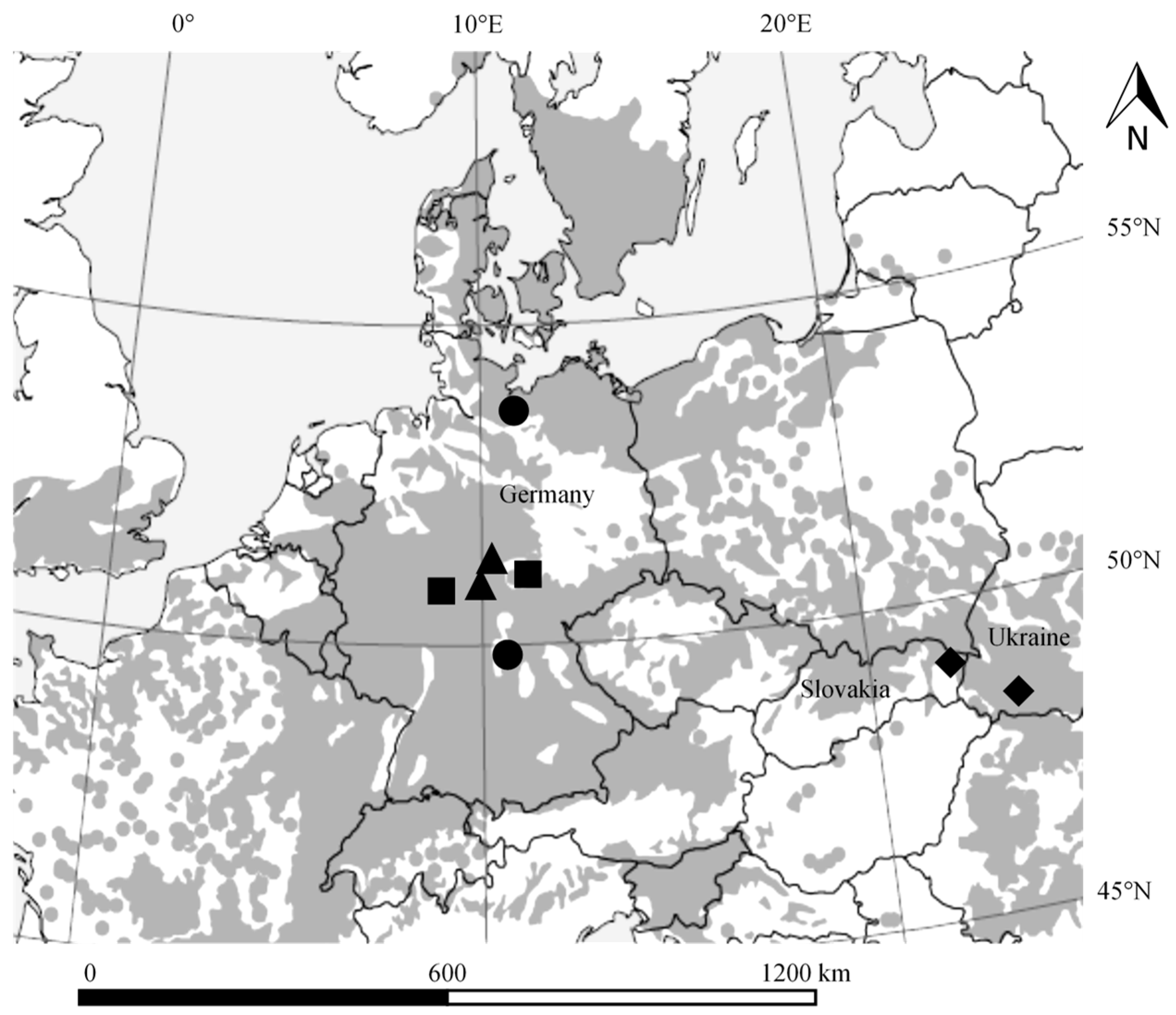
2.1. Study Sites

Eight different study sites (Figure 1 and Table 1) with two study plots each, resulting in a total of 16 beech-dominated forest plots were selected at latitudes between 48° N (Slovakia and Ukraine) and 53° N (Lübeck, Germany; Figure 1 and Table 2). Site selection aimed at similar site conditions and age structure throughout all sites. All plots were located in pure stands of European beech or in beech-dominated stands (at least 66 % basal area represented by beech); in managed forests, most recent interventions dated back at least two years; forest stands were at least in the developmental stage of “mature timber” (>80 years).
The site selection followed a management-intensity gradient from traditionally managed stands, over alternatively managed, lately unmanaged (National Parks) to unmanaged (primary) forests (Figure 1 and Table 1). Stands within the “traditionally managed” group were managed following the “Guidelines of beech forest management in Lower Saxony” [34] which are mainly based on regular thinning cycles of five to ten years and a target diameter harvest around age 120 to 140 years. Stands were chosen in the districts of Hannoversch Münden and Reinhausen (Lower Saxony, Germany).
The “alternative” management group comprised stands with a reduced thinning frequency and intensity. Stands were chosen in the forest districts of Lübeck (Schleswig-Holstein) and Ebrach (Bavaria), both Germany. The management within this group either aimed at higher growing stocks (Lübeck) or a high amount of dead-wood (Ebrach).
Data for lately unmanaged stands was collected in the German National Parks “Hainich” (Thuringia) and “Kellerwald-Edersee” (Hesse). Management has been ceased in both areas for two to three decades.
Two sites in the primary beech forests of the Carpathian Mountains were chosen as unmanaged forests. One was located in Rožok, Slovakia, a highly protected reserve near the Ukrainian border. The other was in Uholka in the Ukrainian Uholka-Shyrokoluzhansky area, belonging to the Carpathian Biosphere Reserve. More information on the sites can be found in Stiers et al. [35] and Willim et al. [36].

2.2. Sampling Design and Data Collection (Terrestrial Laser Scanning)

Within the selected stands, canopy gaps and associated regeneration patches were detected and recorded following pre-defined transect lines [35,36]. To ensure comparability between different regeneration patches, the age of the regeneration was estimated by counting internodes and was not to exceed 10–15 years. Additionally, the regeneration area was not to be larger than 50 m × 50 m (2500 m2) to ensure that a complete capture with terrestrial laser scans was possible.
In each forest a plot with an area of 50 m × 50 m was scanned with a Faro Focus 3D 120 or a Faro Focus M70 (both Faro Technologies Inc., Lake Mary, FL, USA) terrestrial laser scanner, depending on instrument availability. For both instruments, scan settings were set to cover a field of view of 360° in horizontal and 300° in vertical direction with an angular resolution of 10.240 points per 360° with the scanner mounted on a tripod at breast height (1.30 m). Using phase-difference technology the scanners measured the distance to surrounding trees or other vegetation elements with a maximum distance of 70 (M70) to 120 m (Focus 120). All scans were conducted in the vegetation periods 2017 and 2018, with all species being densely foliated. In total, 30–80 scans were performed in each plot, depending on the density of the understory vegetation, to ensure capture of every object in the plot with greatest possible detail from several directions and with minimized shadowing [38]. For spatial co-registration of the scans with Faro-Software Faro Scene, we evenly distributed 70–90 artificial checkerboard targets throughout the plot. In cases of high regeneration density, it cannot be excluded that there was a shadowing effect in the data (despite very large numbers of scan positions). This could possibly have led to an underestimation of plants in the gap centers or other densely covered areas. To filter for erroneous points according to the standard settings and for the registration we used Faro Scene Software (Faro Technologies Inc., Lake Mary, FL, USA, Version 7.1.1.81).

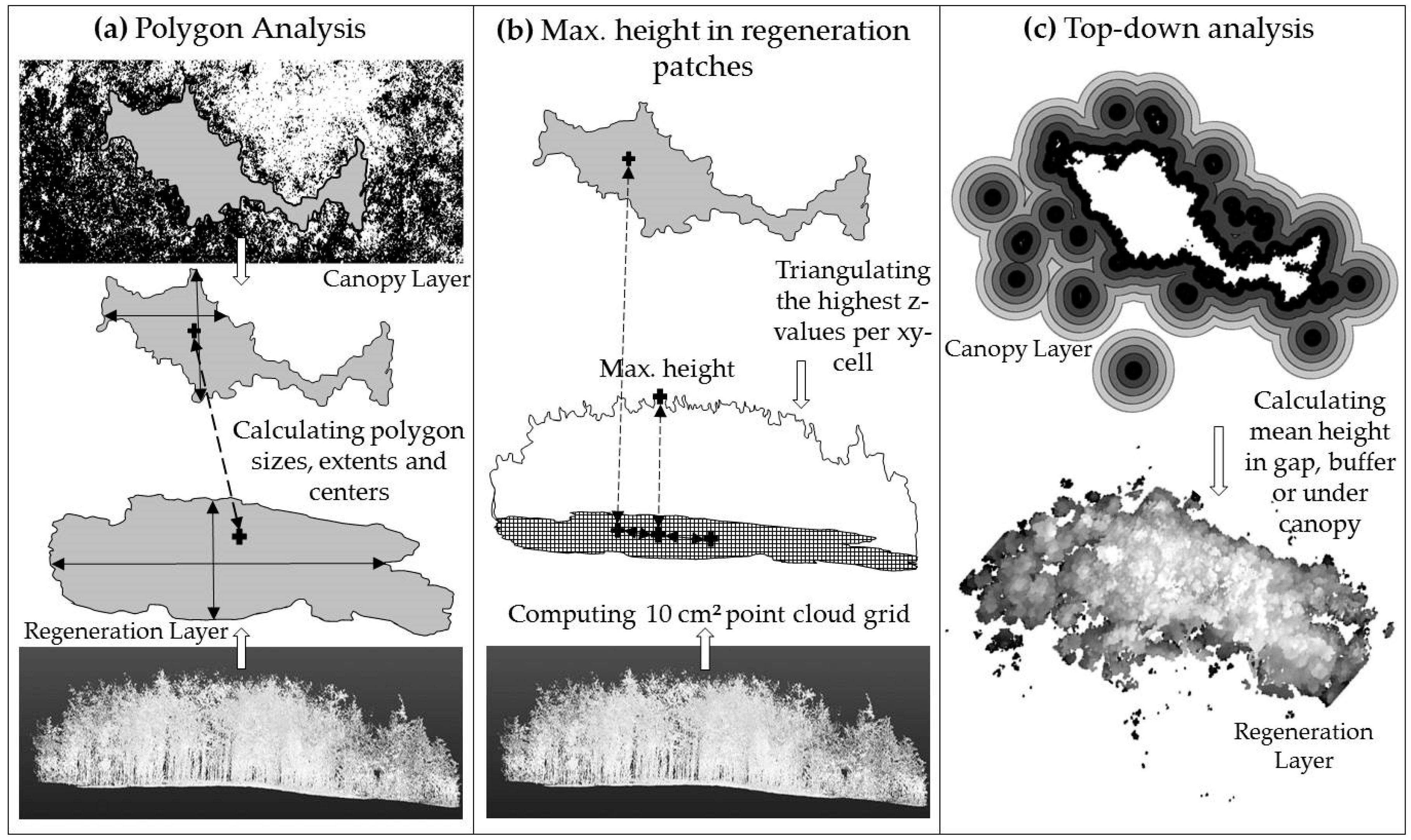
2.3. Data Analysis of Gap and Understory Characteristics—Size, Shape and Center

Considering the large number of slightly different gap definitions, we decided to define a canopy opening as canopy gap, when its vertical extension reaches down through all crown layers to a height above ground of at least one third of dominant tree height or below. To sufficiently describe gaps, size, shape and age are important parameters affecting the ecological impact of the respective gap [11]. The data was analyzed following three different approaches (Figure 2). To calculate and identify shape and size characteristics of the gaps and regeneration patches, as well as availability of direct radiation in canopy gaps, we used delineated polygons of gap and regeneration patch area (Figure 2a). To identify the maximum regeneration height within the regeneration patches, we computed a point cloud grid [39] with a resolution of 10 cm for each regeneration patch and analyzed the offsets between projected gap center and maximum height of the regeneration, and between regeneration patch center and maximum height of the regeneration (Figure 2b). Raster data that referred to subsamples of every 50 m × 50 m plot was used for a top-down analysis of overstory and regeneration dependency. This was conducted to figure out whether the regeneration height differed between the locations directly within the gap polygon or under the canopy (Figure 2c).
After combining the single scans into the final multi-scan point cloud, the point cloud was separated into a regeneration layer and a canopy layer (Figure 2a) using one third of the dominant tree height as height threshold consistent with our gap definition. For both “layers” we created a separate xyz-file for further processing. In order to identify the canopy gaps in the point clouds we assigned two different colors to regeneration and overstory using the two separate files. After coloring the point clouds both files were looked at from bird’s eye perspective and the outline of the gap was manually delineated. Then, the area (m2) of the canopy gaps was computed using Delaunay-Triangulation (maximal triangle side length: 0.25 m) in Cloud Compare (Version 2.8.1, cloudcompare.org, EDF R&D, Paris, France).. The regeneration patch area was also manually delineated by visual assessment.
Since the gap and regeneration polygons had an irregular shape, we compared two methods to determine the center of the gap and regeneration polygons. Firstly, centers were calculated as intersection point of the two lines bisecting the smallest rectangle that encloses the polygon. Secondly, we defined the center of the polygons as the median of the X- and Y- coordinates of the points created during the delineation of the polygons. Because no deviations were found between these variants, only the results of the first method were used afterwards.
While analyzing the associated layers of canopy gaps and regeneration patches it was not always possible to identify a single gap, which solely can be considered responsible for the development of the regeneration patch. In such cases, the areas of all gaps identified in the vicinity of the regeneration were summed up and treated as a single gap during analysis.
The horizontal shift between the projected center of the canopy gap and the regeneration center was calculated by subtracting the respective X- and Y-coordinates (regeneration center – gap center; Figure 2a). By calculating the angle (cos (α)) between the two-dimensional shift-vector and a north-vector as reference, the offset towards North could be analyzed.
To approximate the shape of the canopy gaps, the maximum spatial extent in north–south and west–east directions was calculated (Figure 2a). In order to allow conclusions about the shape, a ratio of the extent in both directions was calculated, comparing the real gap shape to a circular gap. For a regular, circular gap, this ratio was 1. For an irregularly shaped gap, elongated along the north–south axis the ratio took values >1 and along the west–east axis <1. We also calculated the diameter-to-height (d/h) gap-ratio of each gap as a measure to specify the theoretical availability of direct light in the gap. For the calculation of these gap-ratios, we used the spatial extent of each gap in the north–south direction as an indication for the gap diameter as low solar angles and the course of the sun resulted in a higher probability of direct light along the north–south gradient, while height was defined as maximum stand height on plot level. The probability of the incidence of direct light decreased with decreasing gap-ratio.
To analyze the spatial arrangement of plants in relation to the gap or regeneration patch center and to identify the maximum heights within the regeneration patches we computed digital terrain models (DTM) through triangulation of the lowest z-values per 10 cm2 horizontal cell (xy-cell; Figure 2b). We then normalized the point cloud of the regeneration patches by correcting each point in the point cloud with the underlying terrain height obtained from the DTM. After normalizing the point cloud, digital surface models (DSM; top of regeneration) were calculated for the 3D point clouds of the delineated regeneration patches. These DSMs were considered to represent the actual heights of the regeneration patches per xy-cell. To calculate the position of the maximum height within the regeneration patch, the maximum height was determined for each xy-cell of the point cloud grid (Figure 2b). Thus, the cell with the greatest height was identified and its xy-coordinates captured to calculate the distances to the center of the regeneration patch and the projected gap center as well as the horizontal shifts between these centers and the largest height. This was done as described above for the shift between gap and regeneration center.

2.3.1. Direct Radiation on the Forest Floor

In addition to the gap’s shapes and sizes, there are other important factors that influence the availability of light on the forest floor [5,11,40]. One of these factors is the maximum height of the surrounding forest stand (Figure 3). In order to determine whether direct light could theoretically reach the forest floor under the gap we further approximated the maximum solar angle at each gap using the formula:
Maximum solar angle = 90°-latitude + 23.43°
with 90°-latitude describing the angle between pole and zenith of the site plus obliquity of the ecliptic of the earth. Based on the data of stand height and maximum solar angle it is possible to calculate a minimum diameter which a circular gap must provide to allow direct sunlight to reach the forest floor in the gap. This minimum diameter was calculated using the Theorem of Pythagoras. To estimate whether direct radiation could potentially reach the forest floor we used the maximum extent of the gap (maximum length of a traverse).

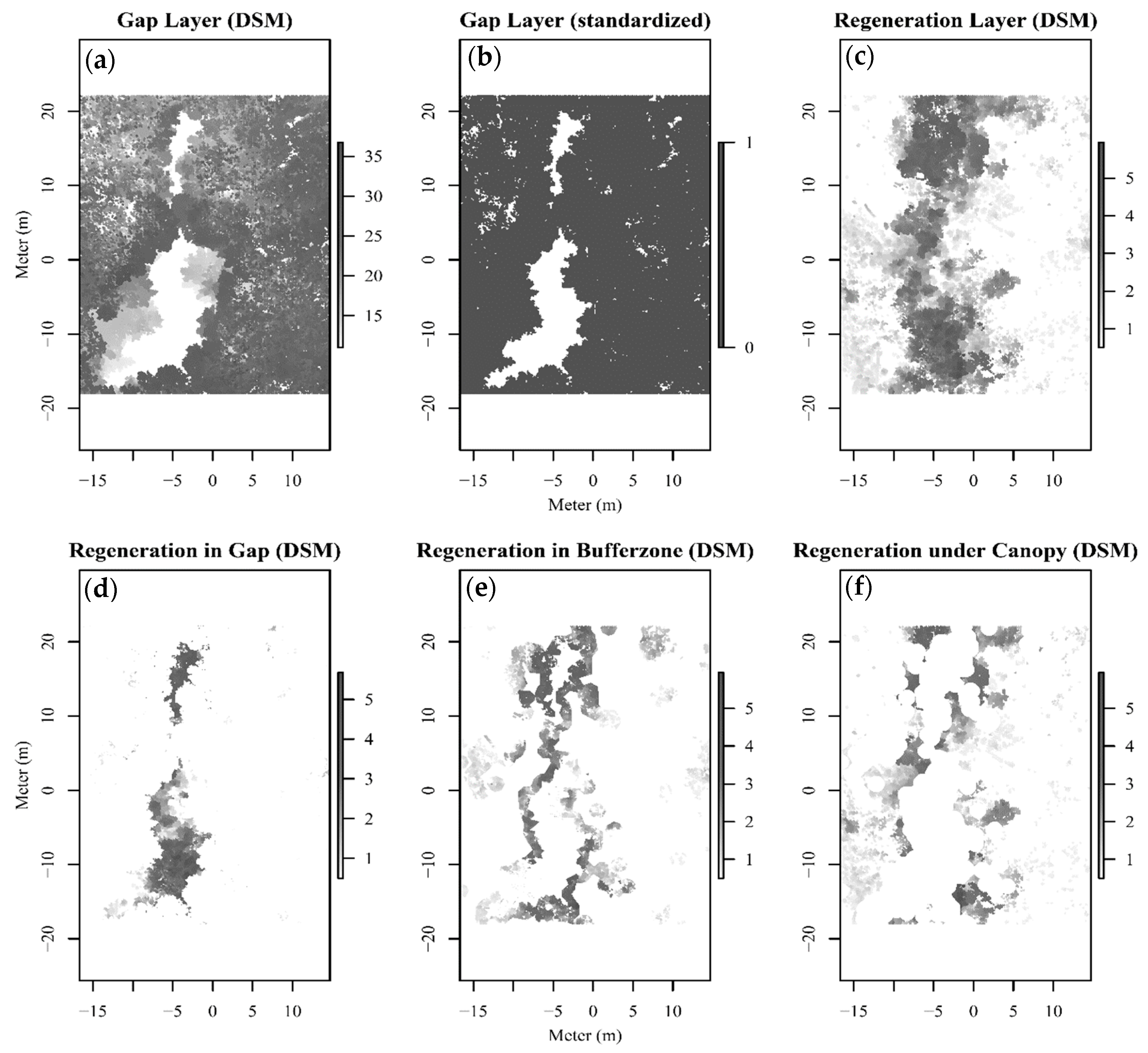
2.3.2. Top-Down Analysis

The term top-down relationship is defined as the dependency of the understory layers on the canopy within a forest (compare above). Here, we especially focus on the spatial link between these layers. We used a top-down dependency analysis to address hypothesis (b), namely whether the height values of the regeneration patches are influenced by a position in the gap polygon or under the canopy (Figure 2c). In the first step, the whole multi-scan point clouds were transformed into a point cloud grid of 10 cm resolution. The further analysis refers to subsamples of every transformed multi-scan point cloud by virtually cutting out one rectangular subarea per plot that contains the understory and as many canopy openings as possible. These rectangular subunits of the plots were further subdivided into two layers. The height of each layer was determined by the total stand height in the respective forest scene (Table 2). The bottom layer, referred to as “regeneration layer” reached from 0 m (normalized forest ground) to one third of stand height. The upper layer, referred to as “canopy layer” consisted of all remaining points.
The regeneration layers were further processed to determine understory heights. To do so, first we excluded all xy-cells of the point cloud grid with heights (z-values) lower than 0.5 m to avoid misinterpretations of dead wood, herbs, shrubs, ferns and grasses. Furthermore, stems and low-hanging branches of upper layers were also removed from the point cloud grid (manually) to avoid effects of overstory tree elements before deriving heights (maximum z-value) for each xy-cell in the understory layer.
In the next step, digital surface models (DSM) of both layers were computed (Figure 4a,c) as well as a standardized 1/0-grid for each canopy layer, which was “1” when a canopy element was above the observed xy-cell and “0” when there was none (Figure 4b).
In the final steps, the canopy and regeneration raster layers were merged respectively for each plot, and the regeneration was separated into saplings located in the gap (Figure 4d) and saplings beneath closed canopy (Figure 4f).
To also consider a penumbral zone, which is the adjacent area around a canopy gap that is still affected by canopy opening due to an increase in light levels [41], we defined five buffer zones around the actual gap projection area with a width of 1 m each (0–1 m; 1–2 m; 2–3 m; 3–4 m; 4–5 m) (e.g., buffer zone 1 (0–1 m); Figure 4e). The term “under closed canopy” may be misleading as the regeneration in the buffer zones was already beneath closed canopy as well. Here, “under closed canopy” stands for regeneration heights that were neither part of the gap nor the defined buffer zones. This was done to specifically compare regeneration areas in the zone of transition between the gap and the closed stand surrounding it.

2.4. Statistical Analysis

We used parametric or non-parametric tests to analyze the data, depending on whether parametric assumptions (normal distribution and homogeneity of variance) were fulfilled (Shapiro–Wilk test for normality and Levene test for homogeneity of variance). If all parametric assumptions were met, we used one-way ANOVA, whenever these could not be confirmed the Kruskal–Wallis ANOVA was applied as a non-parametric test. For posthoc comparisons between the different variables we used parametric TukeyHSD test or nonparametric Mann–Whitney–U test. This way, we tested for significant differences between gap sizes among the types of management. Concerning regeneration heights, we tested for significant differences depending on the position of the regeneration area. The latter was tested for each plot, each type of management, and the full dataset. Furthermore, we tested for significant differences in height decline from within-gap positions over transition zone to positions under canopy on plot level. To analyze the relationship between gap size and regeneration patch area we used a linear regression model. The raster data was created with the R package “lidR” [42] and analyzed with the R package “raster” [43]. For all statistical tests, we used a significance level of p < 0.05. The statistical analyses were conducted with R [44].

3. Results

3.1. Gap, Understory and Light Regulating Characteristics

In total, we measured extents and gap characteristics of 36 canopy gaps (Table 2). Gap size varied between 85.76 m2 in Hainich National Park and 439.98 m2 in the Rožok primary forest. We found no significant differences in mean gap size between the types of management (F = 1.846, df =3). Mean size of all investigated gaps was 234.31 m2, with only four gaps larger than 400 m2 whilst the mean area under regeneration was 604.40 m2, with the biggest values in primary forests (mean = 910.02 m2), and the lowest area in one of the sites of alternative management (mean = 205.18 m2).
Gap characteristics such as size and maximum extent of the canopy gaps differed considerably between the different forest plots (Table 2). When we tested the relationship between gap size and resulting regeneration area, we found no significant relationship between gap size and the size of the resulting regeneration area based on the delineated gap and regeneration patch polygons (Figure 5a; p = 0.095, F = 3.19, df = 15). However, the relationship between the sizes of gap and regeneration area became significant concerning the raster data in the top-down analysis (Figure 5b; p = 0.033, F = 5.569, df = 15). The regeneration area increased with increasing gap sizes (Figure 5b).
Gap shapes varied from nearly circular (0.96) (6/36 gaps), to irregularly stretched (30/36 gaps) in the north–south (maximum = 2.92) or west–east (minimum = 0.30) direction, while both were similarly frequent (Table 2).
The maximum stand height had a range between 31.25 m in Kellerwald to 45.50 m in Rožok and the calculated maximum solar angles varied between 60.43° and 65.43° (Table 2). Given the maximum solar angle and the individual stand height for each location, minimum diameters of a hypothetical circular gap arose at which direct solar radiation could reach the forest floor in the gap. This theoretical diameter was lowest in Kellerwald with 16.45 m and highest in Uholka with 20.64 m. Regarding the spatial extent in the north–south direction and stand height for light availability, the gap-ratio varied between 0.12 and 1.19 in our study, and only reached 0.50 on average (Table 2).

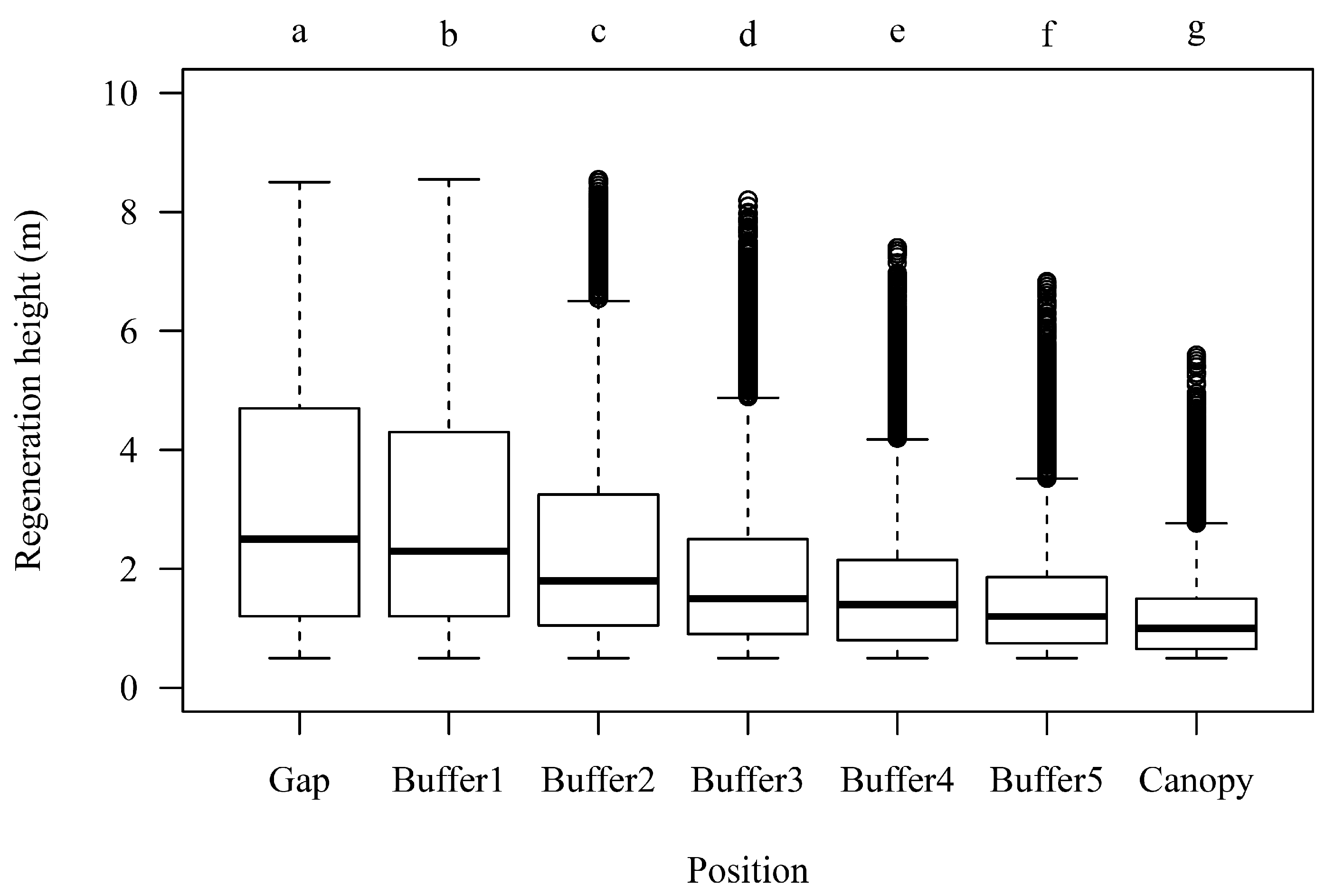
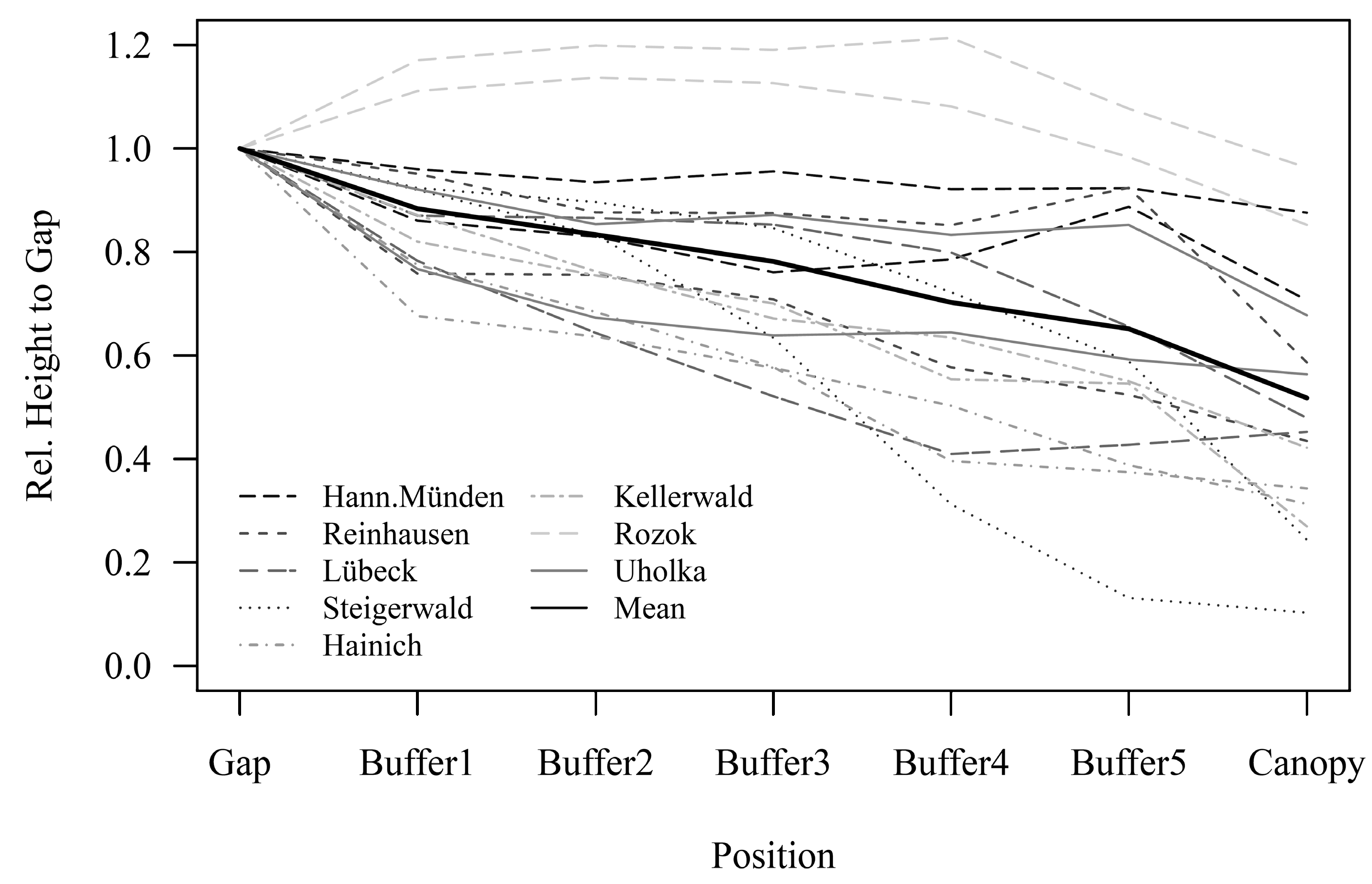
3.2. Regeneration Height in Dependency of Canopy Closure

Depending on the position of the area under regeneration, the top-down analysis revealed the same significant pattern in height decline in total (p = 0.000, F = 15,986, df = 6), for each type of management (Traditional: p = 0.000, F = 884.2, df = 6; Alternative: p = 0.000, F = 4776, df = 6; National Park: p = 0.000, F = 7462, df = 6; Primary forest: p = 0.000, F = 557,9, df = 6), and on plot level (Table 3). Overall, the mean height of the regeneration decreased from positions within the gap, over the five buffer zones, to under densely closed canopy, as defined above (Figure 6).
By analyzing the five buffer zones around the actual gap polygon area separately for each plot, we found a progressive decline in regeneration height from Buffer 1 (up to 1 m distance to the projected gap edge) to Buffer 5 (4–5 m distance to the projected gap edge; Figure 7).
We found the smallest decrease between buffer zones 1–3. The strongest decrease in mean regeneration height (21 %) was found between buffer zone 5 and the regeneration under the closed canopy of the neighboring stand. The differences in mean regeneration height between the outermost buffer zone 5 and the regeneration under the closed canopy were significant for all but four plots (Table 3).

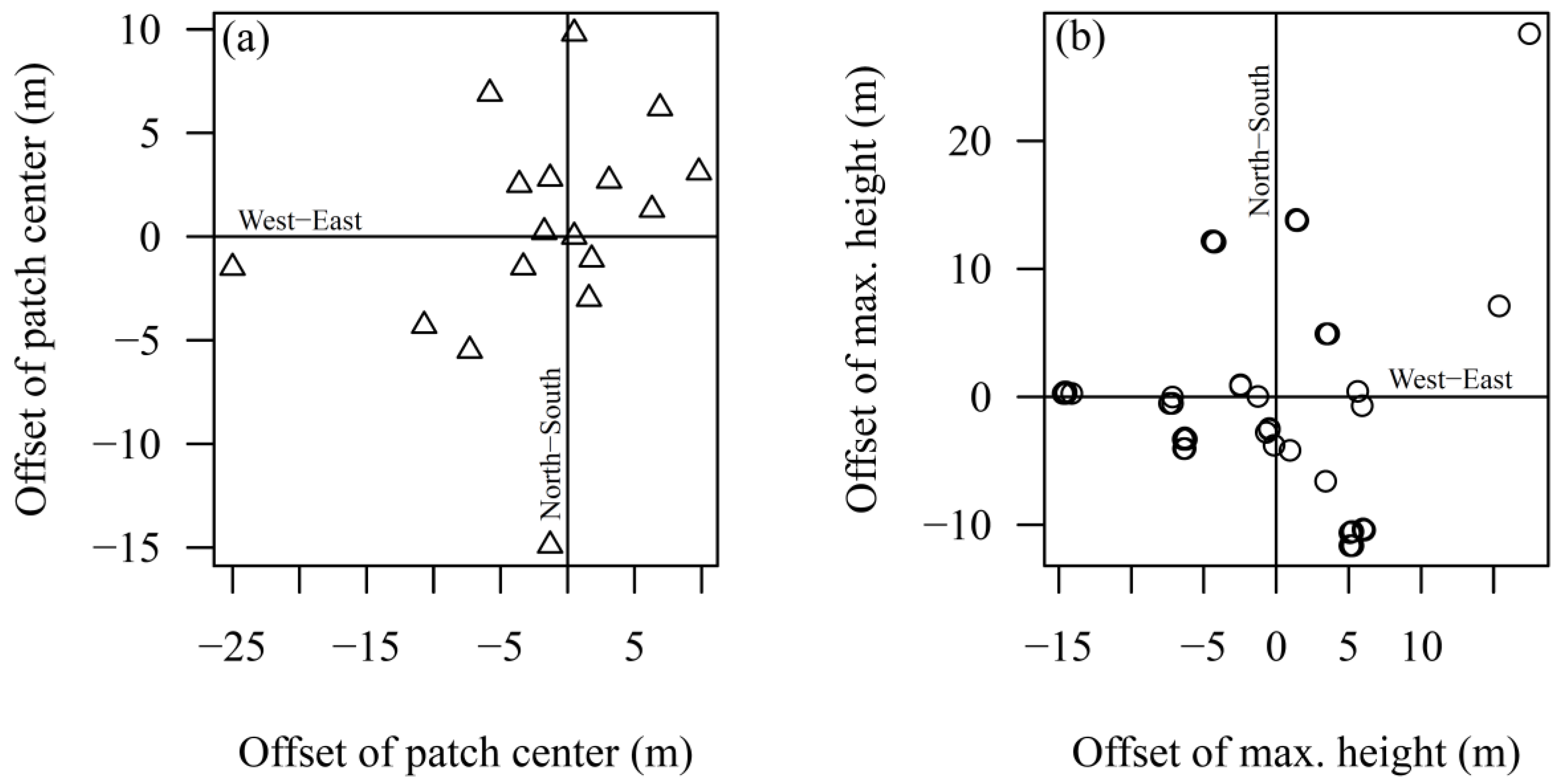
3.3. Spatial Distribution Pattern of Regeneration Areas

There was no uniform pattern in the offset or offset direction of the regeneration patch centers relative to the centers of the gaps. However, the majorities of patch centers were located near the center of the projected canopy gaps (Figure 8a). The mean offset (−1.7/0.2) confirmed the proximity to the gap center. The mean horizontal offset distance between the gap center and the center of the regeneration patch was 7.92 m and varied between 0.5 m and 25.04 m.
Regeneration heights differed significantly within the patch polygons. The maximum height was mainly not measured directly in the projected gap center, but showed an average offset of 10.07 m between maximum height and patch center (Figure 8b). This offset varied between 2.5 m and 33.34 m. Even though the mean regeneration height showed significant differences within the regeneration patch polygon, the mean height values varied only between 1.38 m (minimum at the maximum distance from the gap center) and 2.23 m (maximum at a distance of about 30% from the center). In no case, the maximum height was located at the edge or directly in the center of the regeneration patch area.

4. Discussion

4.1. Light Availability

The fraction of direct light that actually reaches the forest floor depends on three different fundamental aspects: (i) the characteristics describing the canopy gap, such as size, shape and orientation, (ii) height and canopy architecture of gap-bordering trees, and (iii) the geographical location of the forest stand [22,40].
Many studies reported an average gap size in temperate forests of less than 1000 m2, caused by the death of one or several trees, while larger gaps are rather rare [9,44,45]. Larger gaps result in drastically changed conditions in the forest ecosystem and a comparison with smaller treefall-gaps becomes hampered [11,12,21]. Often, 1000 m2 is thus specified as maximum gap size (critical size) to be considered in gap studies. Yamamoto [12,13] reported a mean gap size for temperate forests of 30–140 m2, while an average contribution of gaps to the total forest area in beech-dominated forests of 3 %–19 % is reported in the literature [4]. Gaps larger than 400 m2 were considered rare events [4,9,12]. In our study, mean gap size was 234.31 m2, which is similar to mean gap size of 261 m2 recorded for the primary beech forest Kyjov [4]. The smallest single gap (12 m2) was recorded in Reinhausen and the largest gap reached 476 m2 in the primary forest of Uholka. We found no significant differences in gap size of naturally and artificially created gaps caused by logging in the managed forests.
Gap size, however, is just one important attribute when it comes to light availability. For example, a long, narrow and north–south oriented gap may allow as much direct radiation as a smaller circular or elliptically shaped gap [11]. Earlier studies showed that irregularly shaped gaps receive considerably less direct radiation than circular gaps of the same size [5]. Here, we described the shape using the direction-ratio (Table 2), which is the ratio of the maximum north–south to west–east extension. The gaps in our study were mainly stretched or elliptical rather than circular in shape, which affects the amount of incoming direct light. This is crucial as the low solar elevation angles in northern latitudes and the course of the sun result in a drastically limited amount of direct light for narrow gaps orientated west to east. In north–south oriented gaps, the probability of direct radiation on the forest floor was therefore much higher. Another important factor was stand height. The taller the edge trees were, the lower the probability of direct solar radiation in a gap of a given size (Figure 3). In our case, when comparing the maximal spatial extent of the canopy gaps and the theoretical diameter required for receiving direct light through the actual gap opening, direct sunlight could reach the forest floor only in 10 out of the 36 (28 %) gaps.
According to Malcom et al. [22] light-demanding species such as Scots pine (Pinus sylvestris L.), Lodgepole pine (Pinus contorta var latifolia Engelm. Dougl. ex Loud.) and larches (Larix sp.) need a ratio of gap diameter to stand height larger than 2.0 to regenerate. In contrast, intermediate shade-tolerant species such as Douglas fir (Pseudotsuga menziesii (Mirbel) Franco), Sitka spruce (Picea sitchensis (Bong.) Carrière) and Corsican pine (Pinus nigra A.) require gap d/h-ratios between 1.0 and 2.0. Even though gaps with a gap-ratio smaller than 1.0 allow germination for most of the tree species, the low light values in such small gaps permit successful establishment of regeneration for a few shade-tolerant species, e.g., for beech, only [22,26]. Gaps with a ratio less than 0.5 are not appropriate for the establishment of regeneration of any species [46]. These assumptions are, however, not in line with the results presented here. We found established beech regeneration in small gaps with a d/h-ratio as low as 0.12. This highlights that diffuse radiation is clearly sufficient to enable natural regeneration of European beech to establish in low light conditions. The finding that the regeneration patch area showed no increase with increasing d/h-ratio (Table 2) provides further evidence for the independency of early tree regeneration from direct radiation. Thus, the results not only suggest independence of tree regeneration from direct light availability but also confirm once more the high shade-tolerance of European beech compared to other tree species [27,28].

4.2. Spatial Distribution Patterns of Regeneration Height

The availability of light under closed canopies is drastically reduced compared to open-land conditions and increases significantly in gaps [10,18]. It was shown that even treefall gaps with areas between 20–300 m2, as mainly found here, are sufficient to significantly improve the availability of photosynthetic active radiation in the understory [10,21]. However, we did not find a significant relationship between mean sizes of gap and regeneration area when concerning regeneration patch polygons and gap polygons (Figure 5a). Anyhow, we did find a significant relationship between the size of gap openings and the regeneration area, when the analysis was based on the raster data, which represented a more general subsection of the whole plots compared to the delineated polygons (Figure 5b). Thus, our first hypothesis could only be partially confirmed. One possible explanation is the underlying methodology. The comparison between gap size and regeneration patch area was based on a small sample size of 16 forest plots, which were limited to an extent of 50 × 50 m. Furthermore, exact gap age was not known but was only approximated based on the number of visible internodes of the regeneration plants. It was therefore not possible to determine how both the size and the shape of the gaps had changed over time. However, our analyses of buffer zones indicated that the actual regeneration area was generally larger than the associated canopy gap (Figure 6). This emphasizes that the ecological impact of a canopy gap is not limited to the vertically projected area only.
Several studies showed a general increase in height growth of saplings with increased light availability [17,21,22,47,48]. The adjacent forest area, the penumbral zone [41], experiences an increase in light availability due to the canopy opening as well [19]. Using an approach based on buffer zones, which may represent such a penumbral zone, we could confirm our second hypothesis. We found that the mean regeneration height was highest within the gap polygon and declined significantly from the gap edges to the closed canopy (Figure 6 and Figure 7). The significant differences between mean regeneration heights in the gap, the adjacent buffer zone and the neighboring “closed” stand validated the general assumption that regeneration was not only promoted directly in the gap, but also in adjacent parts of the projected gap area. We observed the same pattern of height decline in each of the four management types. Because of significant differences in mean height between regeneration in the outermost buffer zone 5 and the regeneration under closed canopy in at least 12 out of 16 study plots (Table 3), it could be assumed that the penumbral zone had a width of at least 5 m in the investigated managed and unmanaged beech-dominated forests in Central Europe.
The importance of diffuse light for the establishment of beech regeneration may also be the reason why we had to reject hypothesis (c) that suggested an offset of the regeneration patch center towards north. Instead, the regeneration patch centers were located around the gap centers (Figure 8a). This finding is in line with the results of Coates [21] and Malcolm et al. [22] who also found no significant differences between sapling growth in sunny (north edge) and shady (south edge) gap positions for other rather shade-tolerant tree species like spruce (Picea sp.), western hemlock (Tsuga heterophylla), and some fir species (Abies sp.). For more light demanding species, however, contrasting findings have been reported [10,49]. The hypothesized relationship between position and height may only occur in gaps with specific dimensions, where light levels are less uniform across the gap area. For example, Coates [3] found differences in sapling growth of different conifer seedlings from shady southern to sunny northern ends of the gaps, especially in gaps with an area of 300 m2 or more. Hence, it is not surprising that we could not observe a significant shift of the center of the regeneration patch or the maximum height within the patch in any compass direction (Figure 8a,b).
Beside the well-known facts that canopy edge trees do not only respond to changed light regime at the edge of canopy gaps but that they also influence the light availability in the gap themselves [50,51], they affect the belowground resources [52]. Trenching experiments have shown the strong impact of mature trees on regeneration performance by belowground competition [53,54,55]. Height growth of beech seedlings was successfully explained by a combination of above- and belowground resource availability [52]. The lowest amount of root competition induced from the edge trees and a considerable high amount of light availability can be found in the gap center, which suggests good regeneration performance around the gap center. However, in the gap center other factors such as herbaceous competition may also be high [7,56]. This may explain the offset between maximum height and regeneration patch center found in our study suggesting the rejection of our fourth hypothesis. Actually, the maximum height measurements within the regeneration patches were not observed directly in the center, but slightly offset between center and the outer limit of the regeneration patch. Thus, in six out of 16 plots the maximum height of the whole regeneration patch was located in one of the buffer zones and not within the boundaries of the gap polygon. The minimum regeneration heights (mean and in total) were found at the outer edges of the regeneration patches, which may confirm the high competition pressure exerted by the neighboring mature trees. This results in the highest regeneration heights of beech to be found in areas with intermediate light levels, where beech is most competitive [7,57].
All tested hypotheses showed no differences between the four types of management. This shows that after gap creation (be it natural or artificial) regeneration development is driven by management independent factors, presumably most strongly by the abiotic growth site conditions.

5. Conclusions

Even though it is an undisputed fact that the dynamics of natural regeneration are influenced by overstory dynamics such as gap-opening and successive re-closure, these relationships are not easy to quantify. In this study, we found indications for a promotion of beech regeneration beyond gap borders. The fact that regeneration had not only established within the projected gap but also outside of this area confirms that gaps also promote regeneration in parts of the forest stand adjacent to the gap, in the penumbral zone.
A spatial offset northward as reported for several tree species with an assumed lower shade tolerance compared to beech (for example: Sugar maple (Acer saccharum Mrsh.), Western red cedar (Thuja plicata Donn. ex D. Don), Lodgepole pine [3,17,18,21]), could not be confirmed for the shade-tolerant European beech.
Furthermore, it was possible to detect a general pattern of spatial distribution of beech regeneration heights, which seems to be independent of management.
Altogether, these results confirm the importance of canopy gaps and gap dynamics for the establishment and development of natural regeneration, in this case for European beech. We could also show a great potential for regeneration studies based on terrestrial laser scanning. The approach enabled spatial relationships between the overstory and understory to be addressed in a unique way and with great spatial resolution.

Author Contributions

Conceptualization, M.S., K.W., D.S., C.A. and P.A.; data curation, M.S. and K.W.; formal analysis, M.S., K.W., D.S. and P.A.; funding acquisition, D.S., C.A. and P.A.; investigation, M.S., K.W. and M.K.; methodology, M.S., K.W., D.S. and P.A.; project administration, D.S., C.A. and P.A.; supervision, D.S., C.A. and P.A.; writing—original draft, M.S.; writing—review and editing, M.S., D.S., C.A., J.S. and P.A.

Funding

The Erich Ritter Foundation (T0021/29427/2017) is greatly acknowledged for funding this work. The German Research Foundation through grant SE2383/5–1 also funded part of this work.

Acknowledgments

We thank all persons that gave us access to the forest districts they are responsible for and helped us in selection of suitable plots: Axel Pampe, Thomas Schmidt-Langenhorst, Sabine Steinhoff, Knut Sturm, Torsten Welle, Manfred Großmann, Manfred Bauer, Achim Frede, Bernd Schock, Ulrich Mergner, Martin Schafhirt, Peter Jaloviar, and Vasyl Lavnyy. Permits for accessing the primary forests and fieldwork were issued by the responsible environmental protection office in Presov and administration of “Poloniny National park” for Slovakia and Carpathian Biosphere Reserve for Ukraine.

Conflicts of Interest

The authors declare no conflict of interest. The funders had no role in the design of the study; in the collection, analyses, or interpretation of data; in the writing of the manuscript, or in the decision to publish the results.

References

  1. Gustafsson, L.; Baker, S.C.; Bauhus, J.; Beese, W.J.; Brodie, A.; Kouki, J.; Lindenmayer, D.B.; Löhmus, A.; Pastur, G.M.; Messier, C.; et al. Retention forestry to maintain multifunctional forests: A world perspective. BioScience 2012, 62, 633–645. [Google Scholar] [CrossRef]
  2. Nagel, T.A.; Zenner, E.; Brang, P. Research in Old-Growth Forests and Forest Reserves: Implications for Integrated Forest Management. Integrative Approaches as an Opportunity for the Conservation of Forest Biodiversity; European Forest Institute: Freiburg, Germany, 2013; pp. 44–50. [Google Scholar]
  3. Coates, K.D. Tree recruitment in gaps of various size, clearcuts and undisturbed mixed forest of interior British Columbia, Canada. For. Ecol. Manag. 2002, 155, 387–398. [Google Scholar] [CrossRef]
  4. Feldmann, E.; Drößler, L.; Hauck, M.; Kucbel, S.; Pichler, V.; Leuschner, C. Canopy gap dynamics and tree understory release in a virgin beech forest, Slovakian Carpathians. For. Ecol. Manag. 2018, 415, 38–46. [Google Scholar] [CrossRef]
  5. Muscolo, A.; Bagnato, S.; Sidari, M.; Mercurio, R. A review of the roles of forest canopy gaps. J. For. Res. 2014, 25, 725–736. [Google Scholar] [CrossRef]
  6. Meyer, P.; Ammer, C. 6 Anthropogene Störungen 6.1 Waldnutzungen. In Störungsökologie; Wohlgemuth, T., Jentsch, A., Seidl, R., Eds.; UTB GmbH: Stuttgart, Germany, 2019; pp. 273–303. [Google Scholar]
  7. Diaci, J.; Adamic, T.; Rozman, A. Gap recruitment and partitioning in an old-growth beech forest of the Dinaric Mountains: Influences of light regime, herb competition and browsing. For. Ecol. Manag. 2012, 285, 20–28. [Google Scholar] [CrossRef]
  8. Meyer, P.; Tabaku, T.; Lüpke, B.V. Die Struktur albanischer Rotbuchen-Urwälder—Ableitungen für eine naturnahe Buchenwirtschaft. Forstwiss. Cent. 2003, 122, 47–58. [Google Scholar] [CrossRef]
  9. Drößler, L.; von Lüpke, B. Canopy gaps in two virgin beech forest reserves in Slovakia. J. For. Sci. 2005, 51, 446–457. [Google Scholar] [CrossRef]
  10. Canham, C.D.; Denslow, J.S.; Platt, W.J.; Runkle, J.R.; Spies, T.A.; White, P.S. Light regimes beneath closed canopies and treefall-gaps in temperate and tropical forests. Can. J. For. Res. 1990, 20, 620–631. [Google Scholar] [CrossRef]
  11. Schliemann, S.A.; Bockheim, J.G. Methods for studying treefall gaps: A review. For. Ecol. Manag. 2011, 261, 1143–1151. [Google Scholar] [CrossRef]
  12. Yamamoto, S.-I. The gap theory in forest dynamics. Bot. Mag. Tokyo 1992, 105, 375–383. [Google Scholar] [CrossRef]
  13. Yamamoto, S.-I. Forest gap dynamics and tree regeneration. J. For. Res. 2000, 5, 223–229. [Google Scholar] [CrossRef]
  14. Runkle, J.R. Patterns of disturbance in some old-growth mesic forests of Eastern North America. Ecology 1982, 63, 1533–1546. [Google Scholar] [CrossRef]
  15. Brokaw, N.V.L. The definition of treefall gap and its effect on measures of forest dynamics. Biotropica 1982, 11, 158–160. [Google Scholar] [CrossRef]
  16. Runkle, J.R. Guidelines and Sample Protocol for Sampling Forest Gaps; General Technical Report PNW-GTR-283; Forest Service: Washington, DC, USA, 1992. [Google Scholar]
  17. Canham, C.D. Growth and canopy architecture of shade-tolerant trees: Response to canopy gaps. Ecology 1988, 69, 786–795. [Google Scholar] [CrossRef]
  18. Canham, C.D. Different responses to gaps among shade-tolerant tree species. Ecology 1989, 70, 548–550. [Google Scholar] [CrossRef]
  19. Brown, N. A gradient of seedling growth from the center of a tropical rain forest canopy gap. For. Ecol. Manag. 1996, 82, 239–244. [Google Scholar] [CrossRef]
  20. Kneeshaw, D.D.; Bergeron, Y. Canopy gap characteristics and tree replacement in the southeastern boreal forest. Ecology 1998, 79, 783–794. [Google Scholar] [CrossRef]
  21. Coates, K.D. Conifer seedling response to northern temperate forest gaps. For. Ecol. Manag. 2000, 127, 249–269. [Google Scholar] [CrossRef]
  22. Malcolm, D.C.; Mason, W.L.; Clarke, G.C. The transformation of conifer forests in Britain—Regeneration, gap size and silvicultural systems. For. Ecol. Manag. 2001, 151, 7–23. [Google Scholar] [CrossRef]
  23. Collet, C.; Lanter, O.; Pardos, M. Effects of canopy opening on the morphology and anatomy of naturally regenerated beech seedlings. Trees 2002, 16, 291–298. [Google Scholar] [CrossRef]
  24. Mitamura, M.; Yamamura, Y.; Nakano, T. Large-scale canopy opening causes decreased photosynthesis in the saplings of shade-tolerant conifer, Abies veitchii. Tree Physiol. 2008, 29, 137–145. [Google Scholar] [CrossRef] [Green Version]
  25. Wagner, S.; Fischer, H.; Huth, F. Canopy effects on vegetation caused by harvesting and regeneration treatments. Eur. J. For. Res. 2011, 130, 17–40. [Google Scholar] [CrossRef]
  26. Emborg, J. Understorey light conditions and regeneration with respect to the structural dynamics of a near-natural temperate deciduous forest in Denmark. For. Ecol. Manag. 1998, 106, 83–95. [Google Scholar] [CrossRef]
  27. Petriţan, A.M.; von Lüpke, B.; Petriţan, I.C. Effects of shade on growth and mortality of maple (Acer pseudoplatanus), ash (Fraxinus excelsior) and beech (Fagus sylvatica) saplings. Forestry 2007, 80, 397–412. [Google Scholar] [CrossRef]
  28. Petriţan, A.M.; von Lüpke, B.; Petriţan, I.C. Influence of light availability on growth, leaf morphology and plant architecture of beech (Fagus sylvatica L.), maple (Acer pseudoplatanus L.) and ash (Fraxinus excelsior L.) saplings. Eur. J. For. Res. 2009, 128, 61–74. [Google Scholar] [CrossRef]
  29. De Lima, R.A.F. Gap size measurement: The proposal of a new field method. For. Ecol. Manag. 2005, 214, 413–419. [Google Scholar] [CrossRef]
  30. Green, P.T. Canopy gaps in rain forest on Christmas Island, Indian Ocean: Size distribution and methods of measurement. J. Trop. Ecol. 1996, 12, 427–434. [Google Scholar] [CrossRef]
  31. Seidel, D.; Ammer, C.; Puettmann, K. Describing forest canopy gaps efficiently, accurately, and objectively: New prospects through the use of terrestrial laser scanning. Agric. For. Meteorol. 2015, 213, 23–32. [Google Scholar] [CrossRef]
  32. Hobi, M.L.; Ginzler, C.; Commarmot, B.; Bugmann, H. Gap pattern of the largest primeval beech forest of Europe revealed by remote sensing. Ecosphere 2015, 6, 1–15. [Google Scholar] [CrossRef]
  33. Koukoulas, S.; Blackburn, G.A. Quantifying the spatial properties of forest canopy gaps using LiDAR imagery and GIS. Int. J. Remote Sens. 2004, 25, 3049–3072. [Google Scholar] [CrossRef]
  34. NLF (Niedersächsische Landesforsten): Entscheidungshilfen zur Behandlung und Entwicklung von Buchenbeständen. Available online: https://www.nw-fva.de/fileadmin/user_upload/Verwaltung/Publikationen/Merkblaetter/Bu_Nds_Entscheidungshilfen_zur_Behandlung_und_Entwicklung_von_Buchenbestaenden.pdf (accessed on 30. July 2018).
  35. Stiers, M.; Willim, K.; Seidel, D.; Ehbrecht, M.; Kabal, M.; Ammer, C.; Annighöfer, P. A quantitative comparison of the structural complexity of managed, lately unmanaged and primary European beech (Fagus sylvatica L.) forests. For. Ecol. Manag. 2018, 430, 357–365. [Google Scholar] [CrossRef]
  36. Willim, K.; Stiers, M.; Annighöfer, P.; Ammer, C.; Ehbrecht, M.; Kabal, M.; Stillhard, J.; Seidel, D. Assessing understory complexity in beech-dominated Forests (Fagus sylvatica L.)-from managed to primary forests. Sensors 2019, 19, 1684. [Google Scholar] [CrossRef]
  37. EUFORGEN. Distribution Map of Beech (Fagus Sylvatica). 2009. Available online: http://www.euforgen.de (accessed on 28 May2018).
  38. Ehbrecht, M.; Schall, P.; Juchheim, J.; Ammer, C.; Seidel, D. Effective number of layers: A new measure for quantifying three-dimensional stand structure based on sampling with terrestrial LiDAR. For. Ecol. Manag. 2016, 380, 212–223. [Google Scholar] [CrossRef]
  39. Seidel, D.; Beyer, F.; Hertel, D.; Fleck, S.; Leuschner, C. 3D-laser scanning: A non-destructive method for studying above-ground biomass and growth of juvenile trees. Agric. For. Meteorol. 2011, 151, 1305–1311. [Google Scholar] [CrossRef]
  40. Messier, C. Managing light and understory vegetation in boreal and temperate broadleaf-conifer forests. In Silviculture of Temperate and Boreal Broadleaf-Conifer Mixtures; Land Management, Handbook; Comeau, P.G., Thomas, K.D., Eds.; BC Ministry of Forests: Victoria, BC, Canada, 1996; pp. 59–81. [Google Scholar]
  41. Kolari, P.; Pumpanen, J.; Kulmala, L.; Ilvesniemi, H.; Nikinmaa, E.; Grönholm, T.; Hari, P. Forest floor vegetation plays an important role in photosynthetic production of boreal forests. For. Ecol. Manag. 2006, 221, 241–248. [Google Scholar] [CrossRef]
  42. Roussel, J.R.; Auty, D. lidR: Airborne LiDAR Data Manipulation and Visualization for Forestry Applications. R Package Version 2.0.0. 2019. Available online: https://CRAN.R-project.org/package=lidR (accessed on 20 February 2019).
  43. Hijmans, R.J. Raster: Geographic Data Analysis and Modeling. R Package Version 2.6–7. 2017. Available online: https://CRAN.R-project.org/package=raster (accessed on 20 February 2019).
  44. R Core Team. R: A Language and Environment for Statistical Computing; R Foundation for Statistical Computing: Vienna, Austria, 2017; Available online: https://www.R-project.org/ (accessed on 20 February 2019).
  45. Hobi, M.L.; Commarmot, B.; Bugmann, H. Pattern and process in the largest primeval beech forest of Europe (Ukrainian Carpathians). J. Veg. Sci. 2015, 26, 323–336. [Google Scholar] [CrossRef]
  46. Zhu, J.; Matsuzaki, T.; Lee, F.; Gonda, Y. Effect of gap size created by thinning on seedling emergency, survival and establishment in a coastal pine forest. For. Ecol. Manag. 2003, 182, 339–354. [Google Scholar] [CrossRef]
  47. Beaudet, M.; Messier, C. Growth and morphological responses of yellow birch, sugar maple and beech seedlings growing under a natural light gradient. Can. J. For. Res. 1998, 28, 1007–1015. [Google Scholar] [CrossRef]
  48. Brokaw, N.V.L.; Busing, R.T. Niche versus chance and tree diversity in forest gaps. Tree 2000, 15, 183–188. [Google Scholar] [CrossRef]
  49. Runkle, J.R. Gap regeneration in some old-growth forests of the eastern United States. Ecology 1981, 62, 1041–1051. [Google Scholar] [CrossRef]
  50. Schröter, M.; Härdtle, W.; von Oheimb, G. Crown plasticity and neighborhood interactions of European beech (Fagus sylvatica L.) in an old-growth forest. Eur. J. For. Res. 2012, 131, 787–798. [Google Scholar] [CrossRef]
  51. Seidel, D.; Ruzicka, K.J.; Puettmann, K. Canopy gaps affect the shape of Douglas-fir crowns in the western Cascades, Oregon. For. Ecol. Manag. 2016, 363, 31–38. [Google Scholar] [CrossRef]
  52. Wagner, S.; Madsen, P.; Ammer, C. Evaluation of different approaches for modelling individual tree seedling height growth. Trees 2009, 23, 701–715. [Google Scholar] [CrossRef] [Green Version]
  53. Riegel, G.M.; Miller, R.F.; Krueger, W.C. Competition for resources between understory vegetation and overstory Pinus ponderosa in northeastern Oregon. Ecol. Appl. 1992, 2, 71–85. [Google Scholar] [CrossRef]
  54. Ammer, C. Response of Fagus sylvatica seedlings to root trenching overstory Picea abies. Scand. J. For. Res. 2002, 17, 408–416. [Google Scholar] [CrossRef]
  55. Petriţan, I.C.; von Lüpke, B.; Petriţan, A.M. Effects of root trenching of overstorey Norway spruce (Picea abies) on growth and biomass of underplanted beech (Fagus sylvatica) and Douglas fir (Pseudotsuga menziesii) saplings. Eur. J. For. Res. 2011, 130, 813–828. [Google Scholar] [CrossRef]
  56. Modrý, M.; Hubený, D.; Rejšek, K. Differential response of naturally regenerated European shade tolerant tree species to soil type and light availability. For. Ecol. Manag. 2004, 188, 185–195. [Google Scholar] [CrossRef]
  57. Rozenbergar, D.; Mikac, S.; Anic, I.; Diaci, J. Gap regeneration patterns in relationship to light heterogeneity in two old-growth beech-fir forest reserves in South East Europe. Forestry 2007, 80, 431–443. [Google Scholar]
Figure 1. Geographic locations of the eight study sites with their management regimes (▲ = traditionally managed, ● = alternatively managed, ■ = National Parks, ♦ = primary forests; modified after Stiers et al. [35]) in relation to the potential natural vegetation (grey) of European beech without human influence according to the European Forest Genetic Resources Programme (EUFORGEN) [37].
Forests 10 00637 g001
Figure 2. Illustration of the three different approaches used in this study. (a) Data analysis to calculate polygon sizes, maximum extents and center positions based on manually delineated polygons. (b) Computing 10 cm point cloud grids to identify the maximum height within the regeneration patches. (c) Top-down analysis based on raster data of 10 cm2 resolution to analyze the top-down dependency.
Forests 10 00637 g002
Figure 3. Schematic representation of the relationship between stand height (h) and maximum solar angle (α) and the resulting minimum diameter (d) of the canopy gap to allow incidence of direct sunlight.
Forests 10 00637 g003
Figure 4. Exemplary maps of horizontal (xy)-cells based on the point cloud grid of a plot, here from one of the Hainich sites. Digital surface models of gap layer (a) and regeneration layer (c), standardized 0/1 canopy layer showing the gap (b). (df): Elements of the regeneration layer located in the gap (d), in a buffer zone of 1 m around regeneration in gap (e) (here exemplary buffer zone 0–1 m), and (f) remaining regeneration under densely closed canopy. DSM = digital surface model.
Forests 10 00637 g004
Figure 5. Scatterplots of regeneration area (m2) over gap size (m2). (a) Non-significant relationship between gap size and resulting regeneration area based on polygon analysis. (b) Significant relationship between gap size and regeneration area based on raster data in top-down analyses. The dashed grey lines mark the 1:1 relationship between both sizes.
Forests 10 00637 g005
Figure 6. Box–whisker plots of the regeneration vegetation height (m) in dependence of position in gap, in buffer zone (1–5 m) or under closed canopy. Different lower-case letters indicate significant differences between positions at the level of p < 0.05.
Forests 10 00637 g006
Figure 7. The different lines illustrate the mean height development of the regeneration relative to height in gap measured for seven classes; Gap = heights within the gap polygon; Buffer 1–5 = subsequent 1 m buffer zones around the gap polygon; Canopy = all remaining heights under the canopy. Each line represents one of the 16 study plots; the solid black line shows the mean height decrease of all plots together.
Forests 10 00637 g007
Figure 8. Horizontal shift (a) of the regeneration patch center relative to the center of the canopy opening (0/0), respectively and (b) horizontal shift of the maximum height within the regeneration patch relative to the center of the regeneration patch (0/0), respectively. Open triangles mark the position {x/y} of the regeneration patch center (a) and open circles mark the maximum height within the patch (b). The point (0/0) in the two-dimensional coordinate system is equivalent to the projected center of the canopy gap (a) or the center of the regeneration patch (b).
Forests 10 00637 g008
Table 1. Detailed information about the climatic and geographic conditions of the study areas and the average age of the studied stands. MAT = mean annual temperature; MAP = mean annual precipitation.
CountryManagement TypeStudy SitesMAT (°C)MAP (mm)Elevation (m a.s.l.)Stand Age (years)
GermanyTraditionally managedHann. Münden6.5–7.5750–1050270–41081
Reinhausen8740190–31098
Alternatively managedEbrach7–8850320–480111
Lübeck8–8.5625–72540–90131
National Park (lately unmanaged)Kellerwald6–8600–800540–635184
Hainich7–8600–800330–380183
SlovakiaPrimary forest (unmanaged)Rožok6–7780580–745Uneven-aged
UkraineUholka 71407700–840Uneven-aged
Table 2. Detailed information about latitude, maximum solar angle, stand height and the theoretical, minimum diameter of a circular gap at which the solar radiation directly hits the forest floor, maximum regeneration height, sizes of regeneration areas and canopy gaps, as well as a description of the spatial extent of the canopy gaps in north-south (NS) or west-east directions (WE). Every time there are multiple values of gap area for one plot, several small gaps were summed-up in terms of canopy opening size, which then was the basis for averaging gap sizes and further analysis.
Study AreaManagement TypeLatitudeMax. Solar AngleMin. Diameter (m)PlotStand Height (m)Canopy Gap (m2)Gap Ratio (d/h)Max. Extension (m)Direction-ratio (NS/WO)Regeneration Area (m2)Max. Height (m)
NSWE
Hann. MündenTraditional51°62.43°17.20134.50 169.211.1138.313.12.92775.763.6
231.4068.290.227.023.40.30748.774.5
78.220.5115.912.41.28
ReinhausenTraditional51°62.43°17.13132.40 17.100.155.06.00.83266.713.9
36.320.216.79.60.70
11.760.185.94.01.48
17.390.175.54.41.25
56.260.4313.911.61.20
31.060.258.08.80.91
26.490.134.110.10.41
233.20107.750.5819.313.01.48332.873.6
EbrachAlternative49°64.43°18.11137.85 175.270.4918.420.60.89335.697.5
125.620.4115.713.81.14
193.130.8231.028.41.10
237.8441.840.176.515.60.42429.088.6
26.240.124.78.00.59
54.370.197.112.00.59
87.740.259.620.80.46
55.980.187.014.70.48
LübeckAlternative53°60.43°19.33133.85 79.650.3512.012.50.96242.045.5
234.29174.340.5920.215.41.31168.334.8
KellerwaldNational Park51°62.43°16.45131.75 246.031.1937.814.12.68587.775.9
231.2594.230.4012.422.50.55931.797.6
96.550.3812.212.70.96
64.780.3711.68.31.40
HainichNational Park51°62.43°19.63138.45 40.310.249.19.80.93642.795.1
236.75131.210.5821.412.01.78568.665.7
RožokPrimary Forest48°65.43°20.25143.75 112.000.4820.911.91.76975.874.2
66.600.3716.110.61.52
229.040.5122.214.31.55
244.8591.220.3515.617.60.891331.816.5
33.770.177.711.00.70
309.250.4218.925.30.75
38.090.2310.38.31.24
UholkaPrimary Forest48°65.43°20.64145.50 86.120.3917.810.71.66596.195.6
244.80475.680.6127.327.31.37736.217.0
Table 3. Mean regeneration height depending on the position of the regeneration area from within-gap over transitional buffer zones to closed-canopy. Different lower-case letters indicate significant differences between positions at the level of p < 0.05. The degrees of freedom in all statistical tests were six. Column “p” lists the p-values that indicates the significance of the test results. The F-value in column “F” indicates the value of the F-distribution used to calculate the p-value.
Position
LocationPlotGapBuffer1Buffer2Buffer3Buffer4Buffer5CanopypF
Hann. Münden11.17 a1.12 b1.09 c1.12 d1.08 e1.08 e1.03 e0.00028.02
21.63 a1.39 b1.35 c1.24 d1.28 e1.44 e1.15 f0.000358.1
Reinhausen11.89 a1.44 b1.43 b1.34 c1.09 d0.99 e0.82 f0.000906.4
21.34 a1.28 b1.18 c1.18 c1.14 c1.24 a0.79 d0.000214.4
Lübeck12.38 a1.87 b1.53 c1.24 d0.98 e1.20 ef1.08 f0.0001730
21.67 a1.45 b1.45 b1.43 b1.34 c1.09 d0.80 e0.000450.9
Ebrach15.13 a4.74 b4.59 c4.34 d3.70 e3.20 f1.25 g0.0001510
25.54 a5.09 b4.61 c3.51 d1.73 e0.73 f0.57 f0.0001035
Hainich12.63 a1.78 b1.68 c1.57 d1.32 e1.02 f0.82 g0.0001237
22.90 a2.25 b1.99 c1.68 d1.15 e1.09 e0.99 e0.0001370
Kellerwald14.17 a3.63 b3.18 c2.79 d2.64 e2.29 f1.76 g0.0003280
25.41 a4.44 b4.09 c3.79 d2.99 e2.95 e1.46 f0.0003439
Rožok11.20 a1.33 b1.37 c1.35 bc1.29 d1.18 a1.02 e0.000169.9
21.21 a1.41 b1.45 c1.44 cd1.46 c1.29 e1.16 f0.000493
Uholka12.21 a1.69 b1.49 c1.41 d1.42 d1.31 e1.24 f0.0001119
22.99 a2.76 b2.56 c2.61 c2.49 c2.55 c2.03 d0.000167.4

