Interannual and Seasonal Variations in Ecosystem Transpiration and Water Use Efficiency in a Tropical Rainforest

 , ,
, ,
Abstract
1. Introduction
2. Materials and Methods
2.1. Study Site
2.2. Climate and Flux Monitoring
2.3. Daytime Evapotranspiration (ET)
2.4. Water Use Efficiency (WUE)
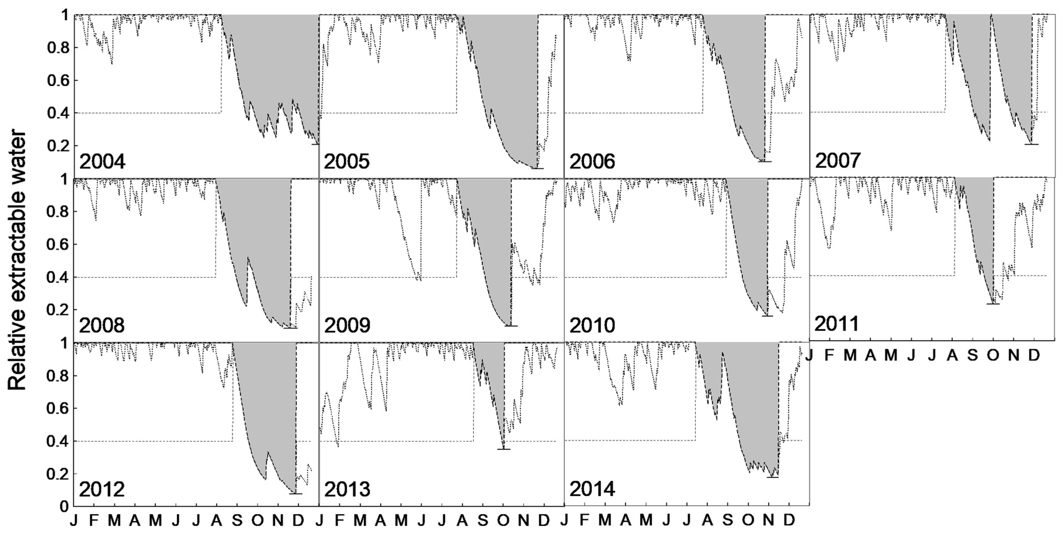
2.5. Soil Water Stress Index (SWSI) and the Water Depletion Period
2.6. Data Analyses
2.6.1. Normalizing ET and WUE
2.6.2. Isolating the Most Important Climate Variables
2.6.3. Ecosystem Response to Climatic Drivers
3. Results
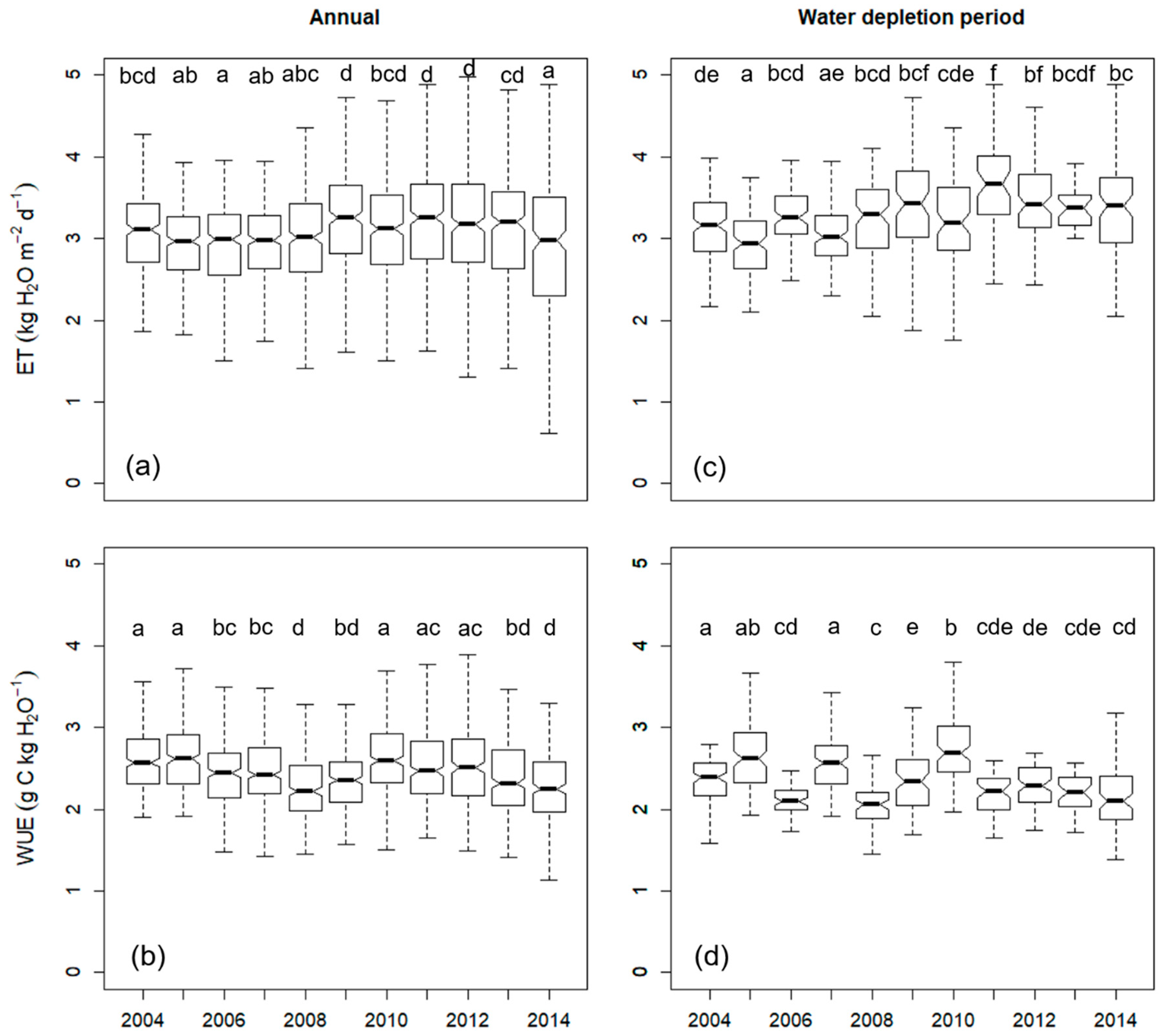
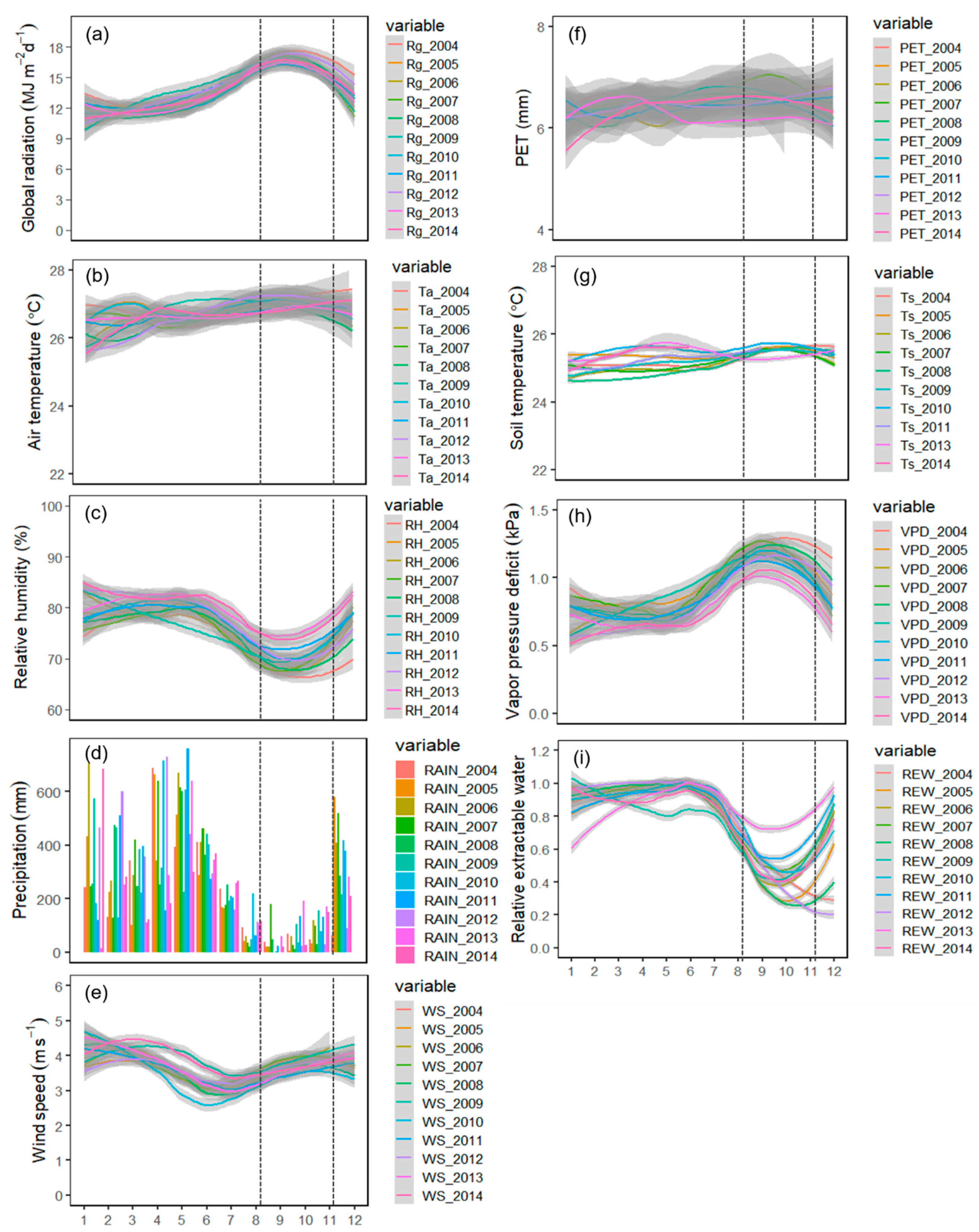
3.1. Interannual Variations in ET, WUE and Climate
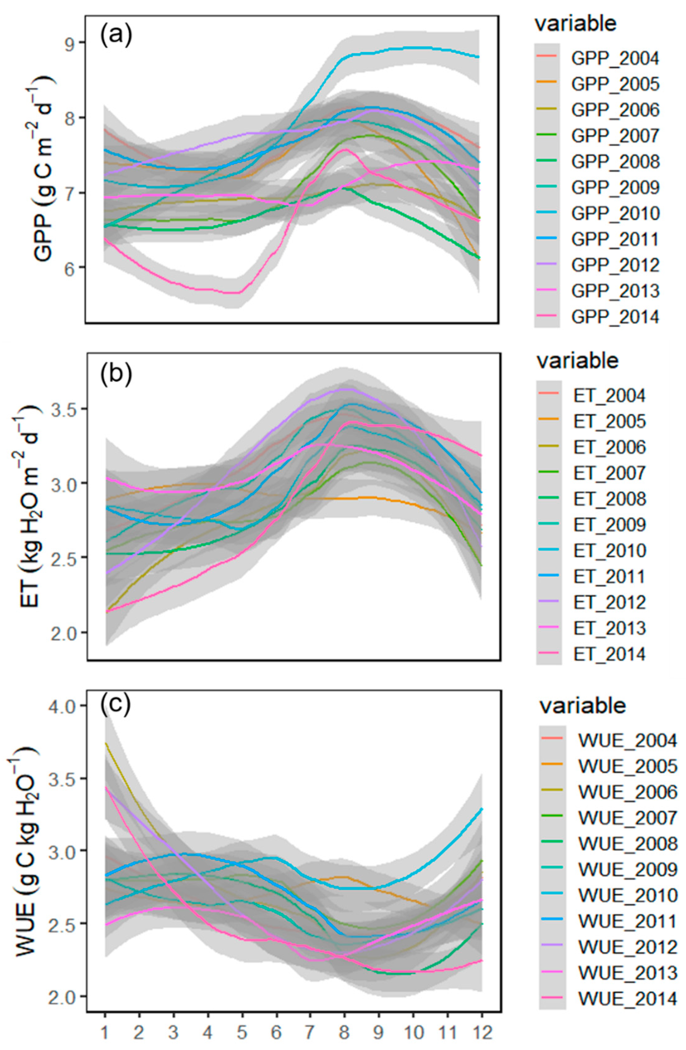
3.2. Seasonal Variations in ET, WUE and climate
3.3. Variations in ET and WUE during the Water Depletion (WD) Periods
4. Discussion
4.1. Interannual Variations in ET and WUE
4.2. Seasonal Variations in ET and WUE
4.3. Variations in ET and WUE within the WD Period
5. Conclusions
Author Contributions
Funding
Acknowledgments
Conflicts of Interest
Appendix A


| Variables | Year | Slope | Slope CI | y-axis Intercept | |
|---|---|---|---|---|---|
| Lower | Upper | ||||
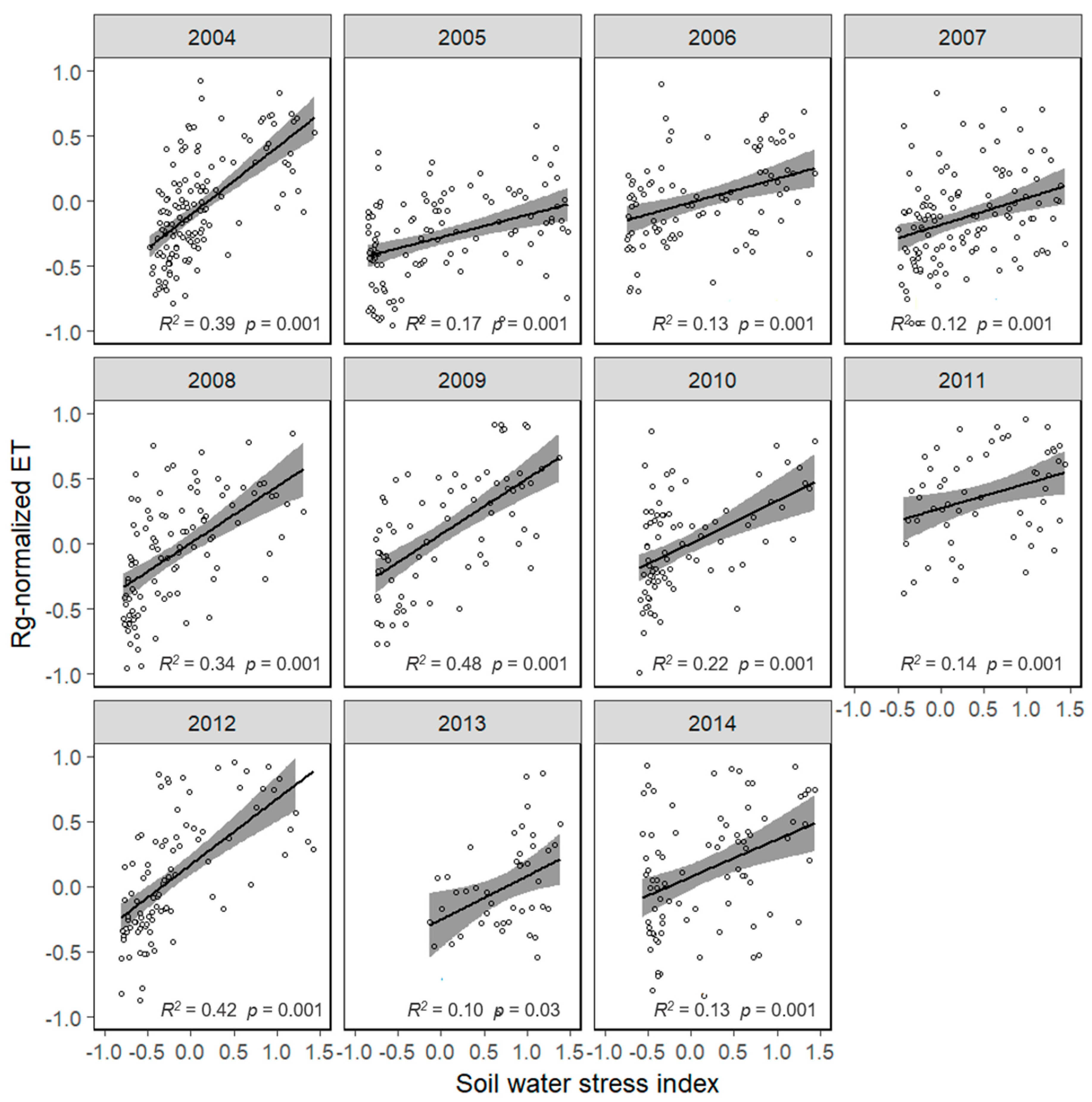
| Rg-Normalized ET and SWSI | 2004 | 0.89 | 0.78 | 1.01 | −0.13 |
| 2005 | 0.46 | 0.39 | 0.54 | −0.28 | |
| 2006 | 0.51 | 0.41 | 0.61 | −0.05 | |
| 2007 | 0.65 | 0.55 | 0.77 | −0.29 | |
| 2008 | 0.81 | 0.69 | 0.94 | 0.07 | |
| 2009 | 0.76 | 0.64 | 0.89 | 0.09 | |
| 2010 | 0.69 | 0.57 | 0.84 | 0.03 | |
| 2011 | 0.63 | 0.49 | 0.80 | 0.07 | |
| 2012 | 0.80 | 0.69 | 0.93 | 0.23 | |
| 2013 | 0.98 | 0.73 | 1.31 | −0.70 | |
| 2014 | 0.86 | 0.70 | 1.04 | 0.04 | |
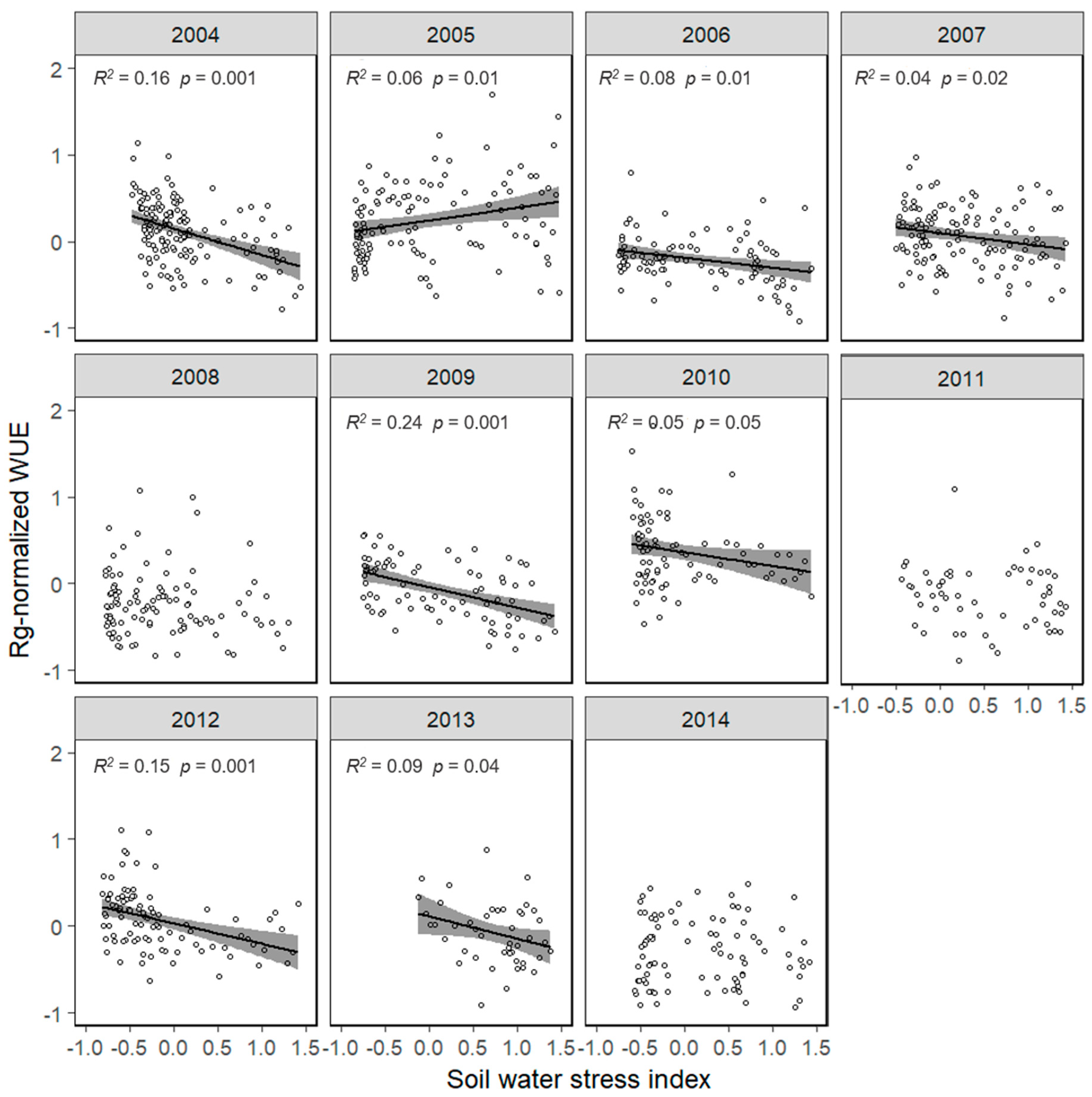
| Rg-Normalized WUE and SWSI | 2004 | −0.75 | −0.87 | −0.64 | 0.18 |
| 2005 | 0.58 | 0.48 | 0.69 | 0.26 | |
| 2006 | −0.40 | −0.49 | −0.33 | −0.16 | |
| 2007 | −0.61 | −0.73 | −0.52 | 0.22 | |
| 2008 | −0.68 | −0.82 | −0.56 | −0.35 | |
| 2009 | −0.48 | −0.58 | −0.39 | −0.01 | |
| 2010 | −0.72 | −0.89 | −0.58 | 0.31 | |
| 2011 | −0.57 | −0.75 | −0.44 | 0.17 | |
| 2012 | −0.60 | −0.73 | −0.49 | −0.04 | |
| 2013 | −0.86 | −1.15 | −0.64 | 0.55 | |
| 2014 | 0.67 | 0.54 | 0.83 | −0.43 | |
| Variables | Comparison of Slopes | |||||||||||
|---|---|---|---|---|---|---|---|---|---|---|---|---|
| 2004 | 2005 | 2006 | 2007 | 2008 | 2009 | 2010 | 2011 | 2012 | 2013 | 2014 | ||
| Rg-Normalized ET | 2004 | |||||||||||
| 2005 | *** | |||||||||||
| 2006 | *** | - | ||||||||||
| 2007 | - | - | - | |||||||||
| 2008 | - | *** | ** | - | ||||||||
| 2009 | - | *** | - | - | - | |||||||
| 2010 | - | - | - | - | - | - | ||||||
| 2011 | - | - | - | - | - | - | - | |||||
| 2012 | - | *** | * | - | - | - | - | - | ||||
| 2013 | - | *** | ** | - | - | - | - | - | - | |||
| 2014 | - | *** | ** | - | - | - | - | - | - | - | ||
| Rg-Normalized WUE | 2004 | |||||||||||
| 2005 | - | |||||||||||
| 2006 | *** | - | ||||||||||
| 2007 | - | - | - | |||||||||
| 2008 | - | - | ** | - | ||||||||
| 2009 | *** | - | - | - | - | |||||||
| 2010 | - | - | *** | - | - | - | ||||||
| 2011 | - | - | - | - | - | - | - | |||||
| 2012 | - | - | - | - | - | - | - | - | ||||
| 2013 | - | - | *** | - | - | - | - | - | - | |||
| 2014 | - | - | ** | - | - | - | - | - | - | - | ||
References
- Von Randow, C.; Zeri, M.; Restrepo-Coupe, N.; Muza, M.N.; de Gonçalves, L.G.G.; Costa, M.H.; Araujo, A.C.; Manzi, A.O.; da Rocha, H.R.; Saleska, S.R.; et al. Interannual variability of carbon and water fluxes in Amazonian forest, Cerrado and pasture sites, as simulated by terrestrial biosphere models. Agric. For. Meteorol. 2013, 182–183, 145–155. [Google Scholar] [CrossRef]
- Duffy, P.B.; Brando, P.; Asner, G.P.; Field, C.B. Projections of future meteorological drought and wet periods in the Amazon. Proc. Natl. Acad. Sci. USA 2015, 112, 13172–13177. [Google Scholar] [CrossRef]
- Cox, P.M.; Betts, R.A.; Collins, M.; Harris, P.P.; Huntingford, C.; Jones, C.D. Amazonian forest dieback under climate-carbon cycle projections for the 21st century. Theor. Appl. Climatol. 2004, 78, 137–156. [Google Scholar] [CrossRef]
- Poulter, B.; Hattermann, F.; Hawkins, E.; Zaehle, S.; Sitch, S.; Restrepo-Coupe, N.; Heyder, U.; Cramer, W. Robust dynamics of Amazon dieback to climate change with perturbed ecosystem model parameters. Glob. Chang. Biol. 2010, 16, 2476–2495. [Google Scholar] [CrossRef]
- Saleska, S.R.; Didan, K.; Huete, A.R.; Da Rocha, H.R. Amazon forests green-up during 2005 drought. Science 2007, 318, 612. [Google Scholar] [CrossRef] [PubMed]
- Phillips, O.L.; Aragão, L.E.O.C.; Lewis, S.L.; Fisher, J.B.; Lloyd, J.; López-González, G.; Malhi, Y.; Monteagudo, A.; Peacock, J.; Quesada, C.A.; et al. Drought sensitivity of the amazon rainforest. Science 2009, 323, 1344–1347. [Google Scholar] [CrossRef] [PubMed]
- Bonal, D.; Burban, B.; Stahl, C.; Wagner, F.; Hérault, B. The response of tropical rainforests to drought—Lessons from recent research and future prospects. Ann. For. Sci. 2016, 73, 27–44. [Google Scholar] [CrossRef] [PubMed]
- Wang, K.C.; Dickinson, R.E. A review of global terrestrial evapotranspiration: Observation, modeling, climatology, and climatic variability. Rev. Geophys. 2012, 50. [Google Scholar] [CrossRef]
- Fisher, R.A.; Williams, M.; da Costa, A.L.; Malhi, Y.; da Costa, R.F.; Almeida, S.; Meir, P. The response of an Eastern Amazonian rain forest to drought stress: Results and modelling analyses from a throughfall exclusion experiment. Glob. Chang. Biol. 2007, 13, 2361–2378. [Google Scholar] [CrossRef]
- Costa, M.H.; Biajoli, M.C.; Sanches, L.; Malhado, A.C.M.; Hutyra, L.R.; Da Rocha, H.R.; Aguiar, R.G.; De Araújo, A.C. Atmospheric versus vegetation controls of Amazonian tropical rain forest evapotranspiration: Are the wet and seasonally dry rain forests any different? J. Geophys. Res. Biogeosci. 2010, 115, 1–9. [Google Scholar] [CrossRef]
- Carswell, F.E.; Costa, A.L.; Palheta, M.; Malhi, Y.; Meir, P.; Costa, J.D.P.R.; Ruivo, M.D.L.; Leal, L.D.S.M.; Costa, J.M.N.; Clement, R.J.; et al. Seasonality in CO2 and H2O flux at an eastern Amazonian rain forest. J. Geophys. Res. D Atmos. 2002, 107, 8076. [Google Scholar] [CrossRef]
- Hasler, N.; Avissar, R. What controls evapotranspiration in the Amazon basin? J. Hydrometeorol. 2007, 8, 380–395. [Google Scholar] [CrossRef]
- Da Rocha, H.R.; Manzi, A.O.; Cabral, O.M.; Miller, S.D.; Goulden, M.L.; Saleska, S.R.; Coupe, N.R.; Wofsy, S.C.; Borma, L.S.; Artaxo, R.; et al. Patterns of water and heat flux across a biome gradient from tropical forest to savanna in brazil. J. Geophys. Res. Biogeosci. 2009, 114. [Google Scholar] [CrossRef]
- Kim, Y.; Knox, R.G.; Longo, M.; Medvigy, D.; Hutyra, L.R.; Pyle, E.H.; Wofsy, S.C.; Bras, R.L.; Moorcroft, P.R. Seasonal carbon dynamics and water fluxes in an Amazon rainforest. Glob. Chang. Biol. 2012, 18, 1322–1334. [Google Scholar] [CrossRef]
- Maeda, E.E.; Ma, X.; Wagner, F.H.; Kim, H.; Oki, T.; Eamus, D.; Huete, A. Evapotranspiration seasonality across the Amazon Basin. Earth Syst. Dyn. 2017, 8, 439–454. [Google Scholar] [CrossRef]
- Farquhar, G.D.; Ehleringer, J.R.; Hubick, K.T. Carbon isotope discrimination and photosynthesis. Ann. Rev. Plant Physiol. 1989, 40, 503–537. [Google Scholar] [CrossRef]
- Hutyra, L.R.; Munger, J.W.; Saleska, S.R.; Gottlieb, E.; Daube, B.C.; Dunn, A.L.; Amaral, D.F.; de Camargo, P.B.; Wofsy, S.C. Seasonal controls on the exchange of carbon and water in an Amazonian rain forest. J. Geophys. Res. Biogeosci. 2007. [Google Scholar] [CrossRef]
- Negrón Juárez, R.I.; Hodnett, M.G.; Fu, R.; Gouden, M.L.; von Randow, C. Control of dry season evapotranspiration over the Amazonian forest as inferred from observation at a Southern Amazon forest site. J. Clim. 2007, 20, 2827–2839. [Google Scholar] [CrossRef]
- Fisher, J.B.; Malhi, Y.; Bonal, D.; Da Rocha, H.R.; De Araújo, A.C.; Gamo, M.; Goulden, M.L.; Rano, T.H.; Huete, A.R.; Kondo, H.; et al. The land-atmosphere water flux in the tropics. Glob. Chang. Biol. 2009. [Google Scholar] [CrossRef]
- Christoffersen, B.O.; Restrepo-Coupe, N.; Arain, M.A.; Baker, I.T.; Cestaro, B.P.; Ciais, P.; Fisher, J.B.; Galbraith, D.; Guan, X.; Gulden, L.; et al. Mechanisms of water supply and vegetation demand govern the seasonality and magnitude of evapotranspiration in Amazonia and Cerrado. Agric. For. Meteorol. 2014, 191, 33–50. [Google Scholar] [CrossRef]
- Da Costa, A.C.L.; Rowland, L.; Oliveira, R.S.; Oliveira, A.A.R.; Binks, O.J.; Salmon, Y.; Vasconcelos, S.S.; Junior, J.A.S.; Ferreira, L.V.; Poyatos, R.; et al. Stand dynamics modulate water cycling and mortality risk in droughted tropical forest. Glob. Chang. Biol. 2018. [Google Scholar] [CrossRef]
- Huang, M.; Piao, S.; Sun, Y.; Ciais, P.; Cheng, L.; Mao, J.; Poulter, B.; Shi, X.; Zeng, Z.; Wang, Y. Change in terrestrial ecosystem water-use efficiency over the last three decades. Glob. Chang. Biol. 2015. [Google Scholar] [CrossRef] [PubMed]
- Brienen, R.J.W.; Wanek, W.; Hietz, P. Stable carbon isotopes in tree rings indicate improved water use efficiency and drought responses of a tropical dry forest tree species. Trees 2011, 25, 103–113. [Google Scholar] [CrossRef]
- Yu, G.; Song, X.; Wang, Q.; Liu, Y.; Guan, D.; Yan, J.; Sun, X.; Zhang, L.; Wen, X. Water-use efficiency of forest ecosystems in eastern China and its relations to climatic variables. New Phytol. 2008, 177, 927–937. [Google Scholar] [CrossRef]
- Aguilos, M.; Hérault, B.; Burban, B.; Wagner, F.; Bonal, D. What drives long-term variations in carbon flux and balance in a tropical rainforest in French Guiana? Agric. For. Meteorol. 2018, 253–254. [Google Scholar] [CrossRef]
- Bonal, D.; Bosc, A.; Ponton, S.; Goret, J.Y.; Burban, B.T.; Gross, P.; Bonnefond, J.M.; Elbers, J.; Longdoz, B.; Epron, D.; et al. Impact of severe dry season on net ecosystem exchange in the Neotropical rainforest of French Guiana. Glob. Chang. Biol. 2008. [Google Scholar] [CrossRef]
- Aubinet, M.; Grelle, A.; Ibrom, A.; Rannik, U.; Moncrieff, J.B.; Foken, T.; Kowalski, A.S.; Martin, P.H.; Berbigier, P.; Bernhofer, C.; et al. Estimates of the annual net carbon and water exchange of forests: The Euroflux methodology. Adv. Ecol. Res. 2000, 30, 113–175. [Google Scholar]
- Wagner, F.; Hérault, B.; Stahl, C.; Bonal, D.; Rossi, V. Modeling water availability for trees in tropical forests. Agric. For. Meteorol. 2011, 151, 1202–1213. [Google Scholar] [CrossRef]
- Kuglitsch, F.G.; Reichstein, M.; Beer, C.; Carrara, A.; Ceulemans, R.; Granier, A.; Janssens, I.A.; Koestner, B.; Lindroth, A.; Loustau, D.; et al. Characterisation of ecosystem water-use efficiency of european forests from eddy covariance measurements. Biogeosci. Discuss. 2008, 5, 4481–4519. [Google Scholar] [CrossRef]
- Dekker, S.C.; Groenendijk, M.; Booth, B.B.B.; Huntingford, C.; Cox, P.M. Spatial and temporal variations in plant water-use efficiency inferred from tree-ring, eddy covariance and atmospheric observations. Earth Syst. Dyn. 2016, 7, 525–533. [Google Scholar] [CrossRef]
- Yang, Y.; Guan, H.; Batelaan, O.; McVicar, T.R.; Long, D.; Piao, S.; Liang, W.; Liu, B.; Jin, Z.; Simmons, C.T. Contrasting responses of water use efficiency to drought across global terrestrial ecosystems. Sci. Rep. 2016, 6, 23284. [Google Scholar] [CrossRef] [PubMed]
- Granier, A.; Bréda, N.; Biron, P.; Villette, S. A lumped water balance model to evaluate duration and intensity of drought constraints in forest stands. Ecol. Model. 1999, 116, 269–283. [Google Scholar] [CrossRef]
- Kume, T.; Takizawa, H.; Yoshifuji, N.; Tanaka, K.; Tantasirin, C.; Tanaka, N.; Suzuki, M. Impact of soil drought on sap flow and water status of evergreen trees in a tropical monsoon forest in northern Thailand. For. Ecol. Manag. 2007, 238, 220–230. [Google Scholar] [CrossRef]
- Xiao, J.; Sun, G.; Chen, J.; Chen, H.; Chen, S.; Dong, G.; Gao, S.; Guo, H.; Guo, J.; Han, S.; et al. Carbon fluxes, evapotranspiration, and water use efficiency of terrestrial ecosystems in China. Agric. For. Meteorol. 2013. [Google Scholar] [CrossRef]
- Boese, S.; Jung, M.; Carvalhais, N.; Reichstein, M. The importance of radiation for semi-empirical water-use efficiency models. Biogeosciences 2017, 14, 3015–3026. [Google Scholar] [CrossRef]
- Bonal, D.; Ponton, S.; Le Thiec, D.; Richard, B.; Ningre, N.; Hérault, B.; Ogée, J.; Gonzalez, S.; Pignal, M.; Sabatier, D.; et al. Leaf functional response to increasing atmospheric CO2 concentrations over the last century in two northern Amazonian tree species: An historical δ13C and δ18O approach using herbarium samples. Plant Cell Environ. 2011, 34, 1332–1344. [Google Scholar] [CrossRef] [PubMed]
- Wagner, F.; Rossi, V.; Stahl, C.; Bonal, D.; Hérault, B. Water availability is the main climate driver of neotropical tree growth. PLoS ONE 2012, 7, e34074. [Google Scholar] [CrossRef]
- Van der Molen, M.K.; Dolman, A.J.; Ciais, P.; Eglin, T.; Gobron, N.; Law, B.E.; Meir, P.; Peters, W.; Phillips, O.L.; Reichstein, M.; et al. Drought and ecosystem carbon cycling. Agric. For. Meteorol. 2011, 151, 765–773. [Google Scholar] [CrossRef]
- Allen, C.D.; Macalady, A.K.; Chenchouni, H.; Bachelet, D.; McDowell, N.; Vennetier, M.; Kitzberger, T.; Rigling, A.; Breshears, D.D.; Hogg, E.H.; et al. A global overview of drought and heat-induced tree mortality reveals emerging climate change risks for forests. For. Ecol. Manag. 2010, 259, 660–684. [Google Scholar] [CrossRef]
- Da Rocha, H.R.; Goulden, M.L.; Miller, S.D.; Menton, M.C.; Pinto, L.D.; De Freitas, H.C. Seasonality of water and heat fluxes over a tropical forest in eastern Amazonia. Ecol. Appl. 2004, 14, 22–32. [Google Scholar] [CrossRef]
- Baldocchi, D.; Falge, E.; Gu, L.; Olson, R.; Hollinger, D.; Running, S.; Anthoni, P.; Bernhofer, C.; Davis, K.; Evans, R.; et al. FLUXNET: A New tool to study the temporal and spatial variability of ecosystem-scale carbon dioxide, water vapor, and energy flux densities. Bull. Am. Meteorol. Soc. 2001, 82, 2415–2434. [Google Scholar] [CrossRef]
- Stahl, C.; Hérault, B.; Rossi, V.; Burban, B.; Bréchet, C.; Bonal, D. Depth of soil water uptake by tropical rainforest trees during dry periods: Does tree dimension matter? Oecologia 2013, 173, 1191–1201. [Google Scholar] [CrossRef] [PubMed]
- Nepstad, D.C.; De Carvalho, C.R.; Davidson, E.A.; Jipp, P.H.; Lefebvre, P.A.; Negreiros, G.H.; Da Silva, E.D.; Stone, T.A.; Trumbore, S.E.; Vieira, S. The role of deep roots in the hydrological and carbon cycles of Amazonian forests and pastures. Nature 1994. [Google Scholar] [CrossRef]
- Lee, J.-E.; Boyce, K. Impact of the hydraulic capacity of plants on water and carbon fluxes in tropical South America. J. Geophys. Res. 2010. [Google Scholar] [CrossRef]
- Xiao, X.; Zhang, Q.; Saleska, S.; Hutyra, L.; De Camargo, P.; Wofsy, S.; Frolking, S.; Boles, S.; Keller, M.; Moore, B. Satellite-based modeling of gross primary production in a seasonally moist tropical evergreen forest. Remote Sens. Environ. 2005, 94, 105–122. [Google Scholar] [CrossRef]
- Wagner, F.H.; Hérault, B.; Bonal, D.; Stahl, C.; Anderson, L.O.; Baker, T.R.; Becker, G.S.; Beeckman, H.; Souza, D.B.; Botosso, P.C.; et al. Climate seasonality limits leaf carbon assimilation and wood productivity in tropical forests. Biogeosciences 2016, 13, 2537–2562. [Google Scholar] [CrossRef]
- Stahl, C.; Burban, B.; Wagner, F.; Goret, J.-Y.; Bompy, F.; Bonal, D. Influence of Seasonal Variations in Soil Water Availability on Gas Exchange of Tropical Canopy Trees. Biotropica 2013, 45, 155–164. [Google Scholar] [CrossRef]
- Maréchaux, I.; Bonal, D.; Bartlett, M.K.; Burban, B.; Coste, S.; Courtois, E.A.; Dulormne, M.; Goret, J.-Y.; Mira, E.; Mirabel, A.; et al. Dry-season decline in tree sapflux is correlated with leaf turgor loss point in a tropical rainforest. Funct. Ecol. 2018, 32, 2285–2297. [Google Scholar] [CrossRef]
- Chaves, M.M.; Maroco, J.P.; Pereira, J.S. Understanding plant responses to drought–from genes to the whole plant. Funct. Plant Biol. 2003, 30, 239–264. [Google Scholar] [CrossRef]


| Year | Soil Water Depletion Duration (no. of days) | SWSIa | Minimum REW |
|---|---|---|---|
| 2004 | 143 | 13.2 | 0.21 |
| 2005 | 119 | −5.60 | 0.06 |
| 2006 | 91 | 11.29 | 0.10 |
| 2007 | 127 | 40.04 | 0.20 |
| 2008 | 110 | −12.11 | 0.09 |
| 2009 | 80 | 11.13 | 0.10 |
| 2010 | 83 | −5.94 | 0.16 |
| 2011 | 57 | 29.97 | 0.23 |
| 2012 | 93 | −17.37 | 0.08 |
| 2013 | 45 | 32.89 | 0.35 |
| 2014 | 122 | 26.65 | 0.17 |
| Period/ | Best Model | Multiple | Intercept | Coefficients | F value | p Value | |
|---|---|---|---|---|---|---|---|
| Dependent Variable | Predictors | R2 | 1 | 2 | |||
| Annual | |||||||
| ET | 0.70 | 2.92 | |||||
| Rg | 0.46 | 0.71 | 1112.9 | <0.001 | |||
| REW | 0.20 | 0.22 | 102.7 | <0.001 | |||
| Ts | 0.06 | 0.04 | 6.8 | <0.001 | |||
| WUE | 0.40 | 2.68 | |||||
| Rg | –0.57 | –0.54 | 164.0 | <0.001 | |||
| REW | 0.09 | –0.08 | 6.9 | <0.001 | |||
| Ts | –0.17 | –0.02 | 2.5 | <0.050 | |||
| Water depletion (WD) period | |||||||
| ET | 0.48 | 3.19 | |||||
| Rg | 9.51 | 3.39 | 180.6 | <0.001 | |||
| REW | 1.01 | 2.20 | 105.3 | <0.001 | |||
| WUE | 0.34 | 2.48 | |||||
| Rg | –0.16 | –0.29 | 86.9 | <0.001 | |||
| Ts | –0.12 | 0.08 | 21.9 | <0.001 | |||
| Location/Ecosystem | Study Period | Interannual Variations in ET (%) | Daily Average ET (kg H2O m−2 d−1) | References | |
|---|---|---|---|---|---|
| Annual Period | Water Depletion Period | ||||
| Southern Brazil, Amazon | 2000–2002 | 5–10 | 2.7 | [18] | |
| Tropical forests mostly Amazon | 3.75 | [19] | |||
| (modelling study) | |||||
| Amazon forests | 1996–2006 | [13] | |||
| -Manaus | 3.3–3.9 | ||||
| -Santarem | 3.3–3.9 | ||||
| -Jaru | 1.3–3.3 | ||||
| -Javaes | 1.3–3.3 | ||||
| -Sinop | 1.3–3.3 | ||||
| -Pe de Gigante | 1.3 | ||||
| Eastern Amazon | 2000–2001 | 3.51 | 3.96 | [40] | |
| Amazon | [10] | ||||
| -Manaus | 1999–2000 | 3.58 | 3.70 | ||
| -Santarem | 2000–2003 | 3.49 | 3.59 | ||
| -Jaru | 2000–2003 | 3.57 | 3.27 | ||
| -Sinop | 2004–2005 | 3.11 | 3.18 | ||
| Amazon forest, Brazil | 2002–2006 | 18 | 2.4–3.76 | 3.41 | [17] |
| Sub-tropical forest in China | 2003–2005 | 15.5 | 2.62 | [34] | |
| Tropical forest in Malaysia | 2000–2009 | 12 | 3.62 | [33] | |
| Tropical forest in | 2004–2014 | 10.4 | 2.95 | 3.23 | This study |
| French Guiana | |||||
© 2018 by the authors. Licensee MDPI, Basel, Switzerland. This article is an open access article distributed under the terms and conditions of the Creative Commons Attribution (CC BY) license (http://creativecommons.org/licenses/by/4.0/).
Share and Cite
Aguilos, M.; Stahl, C.; Burban, B.; Hérault, B.; Courtois, E.; Coste, S.; Wagner, F.; Ziegler, C.; Takagi, K.; Bonal, D. Interannual and Seasonal Variations in Ecosystem Transpiration and Water Use Efficiency in a Tropical Rainforest. Forests 2019, 10, 14. https://doi.org/10.3390/f10010014
Aguilos M, Stahl C, Burban B, Hérault B, Courtois E, Coste S, Wagner F, Ziegler C, Takagi K, Bonal D. Interannual and Seasonal Variations in Ecosystem Transpiration and Water Use Efficiency in a Tropical Rainforest. Forests. 2019; 10(1):14. https://doi.org/10.3390/f10010014
Chicago/Turabian StyleAguilos, Maricar, Clément Stahl, Benoit Burban, Bruno Hérault, Elodie Courtois, Sabrina Coste, Fabien Wagner, Camille Ziegler, Kentaro Takagi, and Damien Bonal. 2019. "Interannual and Seasonal Variations in Ecosystem Transpiration and Water Use Efficiency in a Tropical Rainforest" Forests 10, no. 1: 14. https://doi.org/10.3390/f10010014
APA StyleAguilos, M., Stahl, C., Burban, B., Hérault, B., Courtois, E., Coste, S., Wagner, F., Ziegler, C., Takagi, K., & Bonal, D. (2019). Interannual and Seasonal Variations in Ecosystem Transpiration and Water Use Efficiency in a Tropical Rainforest. Forests, 10(1), 14. https://doi.org/10.3390/f10010014