


Abstract
In constrained nonlinear optimization, we aim to achieve two goals: one is to minimize the objective function, and the other is to satisfy the constraints. A common way to balance these competing targets is to use penalty functions. Suppose that an algorithm generates a descent direction and produces a step that decreases the objective function value but increases the constraint violation—a phenomenon known as the Maratos effect. This leads to the rejection of the full step by the non-smooth penalty function; therefore, superlinear convergence is not preserved. This work leverages a piecewise convexity model to solve the optimal PMU placement. A quadratic objective function is minimized subject to a non-convex equality constraint within box constraints [0, 1] × [0, 1] ⊂ R2. The initial non-convex region is reconsidered as a union of piecewise line segments. This decomposition enables algorithms to converge to a local optimum while preserving superlinear convergence near the solution. An analytical solution is presented using the Karush–Kuhn–Tucker conditions. First-and-second-order optimality conditions are applied to find the local minimum. We show how the Maratos effect is avoided by adopting the piecewise convexity without needing a non-smooth penalty function, second-order corrections or employing the watchdog methods. Simulations demonstrate that the algorithms partially search the space along the line segments—avoiding zig-zag trajectories—and reach (0, 1) or (1, 0), where both feasibility and optimality are satisfied at once.
1. Introduction
Solving nonlinear programming models with Sequential Quadratic Programming (SQP) and Interior Point Methods (IPMs) remains an active area of research [1,2,3,4,5,6,7,8]. These methods often encounter the Maratos effect as they approach local optima upon convergence. The appearance of the Maratos effect can slow convergence speed and lead to step length rejection imposed by non-smooth penalty functions to correct the infeasibility [1,2,3,4,5,6,7,8]. During the iterative process, even if the objective function improves, the line search may reject the unit step that could otherwise lead to a solution due to constraint violations with infeasible iterates [1,2,3,4,5,6,7,8]. Consequently, the convergence rate slows down [1,2,3,4,5,6,7,8]. Second-Order Correction (SOC) steps and the watchdog method are strategies used to mitigate the Maratos effect when a non-smooth penalty function is employed [3].
Alternatively, an exact penalty function can be used to overcome the negative issues of the Maratos effect [4]. The watchdog technique is a type of non-monotone line search that accepts a step if the next step successfully decreases the penalty function, even if it initially causes a temporary increase [4]. SOC involves solving an additional, smaller-scale problem to calculate a correction term that improves the search direction [4,5].
Unconstrained optimization is also the principal domain in both theoretical and practical implementations. It is widely used to solve nonlinear, constrained, and multivariable optimization problems [1,2,3,4,5,6,7,8]. In addition, many recurrent neural networks designed for constrained optimization problems adopt a penalty function to transform the original problem into an unconstrained one [9,10,11,12,13]. A novel multi-agent-based approach for solving the non-convex Economic Dispatch (ED) problem in smart grids is presented in [14]. The authors leverage derivative-free optimization (DFO) methods to enhance performance and facilitate the integration of distributed energy sources through dynamic communication topologies. Novel contributions are presented in nonlinear programming in recent publications [15,16,17,18,19,20,21,22,23,24,25,26,27,28]. Within this broader optimization framework, the Optimal PMU Placement (OPP) problem is a real-world engineering optimization problem, expressed in either the combinatorial or continuous domain [29,30,31,32,33,34,35,36,37,38,39,40,41,42,43,44].
Although the OPP is an NP-complete problem [29,30,31,32], branch-and-bound algorithms can be utilized to solve it [33]. These algorithms provide a global solution within zero-gap optimality [33]. The OPP problem is analogous to the Trade Hub Location and Allocation problem, as both involve optimizing the placement and distribution of resources subject to constraints [38]. Deterministic and heuristic algorithms for single- and multi-channel PMU allocation have been proposed [39], allowing branch-and-bound methods to find global solutions efficiently, with the key aspect of maximum observability covered.
The objective is to minimize the PMU numbers satisfying complete observability along with maximum redundancy [33,34,39,40]. Generalized Pattern Search [40], Genetic Algorithm–based heuristic for comprehensive PMU placement under practical constraints [41], Recursive Tabu Search (RTS) [42], Genetic Algorithms [43], Binary Gravitational Search [44], and Binary Swarm Optimization [45] are heuristic algorithms being applied to the OPP problem solving [46,47]. A semi-definite programming (SDP) model with a linear objective under Linear Matrix Inequality (LMI) constraints and binary decision variables is proposed in [48,49,50,51,52,53].
Integer linear programming (ILP) and cutting planes transform the conic constraints into polytopes [33]. With this way, the problem is solvable with branch-and-bound algorithms adopted to solve the zero-one SDP model, returning global solutions [33].
Weighted Least Squares (WLS) algorithms [54], Sequential Quadratic Programming (SQP) [55,56,57,58,59] and Interior-Point Methods (IPMs) [59] (both approaches discussed in [59]) are used to solve nonlinear OPP models giving a least number of PMUs along with PMU locations around the grid [33]. Groebner bases [60] are also applied to OPP problem-solving. A strategic PMU placement using a CNN, improving line outage detection is proposed in [61]. Some novel approaches integrated the OPP solution with a state estimation and power flow analysis in [62,63,64,65,66,67,68,69,70,71,72]. A Wide-Area Monitoring System is constituted by PMUs and Phasor Data Concentrators (PDCs). PMUs provide high-accuracy, time-synchronized measurements, while PDCs aggregate data centrally or at the edge, enhancing latency and bandwidth efficiency [62,63,64,65,66,67,68,69,70,71,72].
Building on distributed economic operations, the integration of PMUs is crucial for real-time monitoring and control. PMUs provide accurate, time-synchronized data, enhancing the effectiveness of distributed optimization algorithms, as discussed in [73]. By incorporating PMU data, the proposed model-based and model-free approaches can better handle system dynamics, improve coordination of distributed energy sources, and optimize electric vehicle charging/discharging schedules under uncertainty.
To adopt a nonlinear model for solving the OPP problem, we often face the challenge of avoiding the Maratos effect [74], in order to ensure optimality while maintaining superlinear convergence near the solution [59]. SOC steps and the watchdog method are remedies employed to avoid the Maratos effect when a non-differentiable penalty function is used [4]. Our approach offers a remedy based on a geometry-driven optimization method, rather than relying solely on an algorithmic approach [74,75,76,77,78,79,80,81,82,83,84,85,86,87,88].
Building on the idea proposed in our previous work [59], this study refines the piecewise convexity and demonstrates its effectiveness in achieving global-like solutions for the OPP problem while avoiding the Maratos effect [74]. As a result, there is no need to employ non-smooth penalty functions, and the negative impact on superlinear convergence is avoided. The union of piecewise line segments ensures that feasibility and optimality are simultaneously satisfied through the iterations. Consequently, there is no need for trust-region calculations, SOC adjustments, or watchdog methods [74,75,76,77,78,79,80,81,82,83,84,85,86,87,88].
In this context, we address a partially convex programming problem, in which the non-convex structure is reconsidered through a piecewise convexity approach [39,58,59].
This novel approach enables the optimizer to guarantee both feasibility and optimality at convergence. By locally exploring line segments in or convex subsets in , solutions are achieved [59]. Accordingly, we studied the OPP model using a nonlinear formulation in , reflecting a two-bus electric transmission network [89,90,91,92,93]. The nonlinear model is solved using iterative schemes such as SQP and IPM methods [59].
The SQP methods and IPM algorithms are calling via the Fmincon and Ipopt optimizers in MATLAB 2016a [89,90,91]. The algorithms locate local solutions that exhibit global-like behavior, reinforcing the suitability of the proposed nonlinear formulation and aligning with recent research developments [94,95,96,97,98,99,100].
2. Mathematical Nonlinear Programming Formulation
Nonlinear programming methods are based on penalty functions to balance feasibility and optimality, which can distort the descent direction and degrade convergence, especially near the solution. The proposed piecewise convexity model decomposes the feasible region into a union of line segments or convex subregions, which is a geometry-driven optimization, as our foundational designs demonstrated in [33,39,55,58,59].
Consequently, the piecewise convex feasible region permits SQP and IPMs to avoid using penalized terms or correction steps to ensure convergence at a superlinear rate. Therefore, feasibility and optimality are attained simultaneously [39,55,58,59,96].
Within this framework, the feasible region can be considered as a local convexification of the feasible region, bridging the gap between convex optimization and nonlinear programming [3,4]. Let us consider the n-dimension vector . The nonlinear model is stated in as [1,2,3,4,5,6,7,8,39,58,59,74,75,76,77,78,79,80,81,82,83,84,85,86,87,88,96]:
where is a vector of entries . : , , with inequality constraints : [1,2,3,4]. Here, I and E are sets of indices for equality and inequality constraints, respectively [1,2,3,4,5,6,7,8,9,10,11,12,13,14,15,58,59,74,75,76,77,78,79,80,81,82,83,84,85,86,87,88,96].
We assume that the functions and , are real-valued and twice continuously differentiable [1,2,3,4,5]. A vector x ∈ X satisfying all the constraints is a feasible solution to the optimization problem; the collection of all such points builds the feasible region [3]. The NLP problem has a local minimum [1,2,3,4,5,6,7,8,9,10,11,12,13,14,15,16,17]. Quasi-Newton methods have been widely utilized for solving such nonlinear programming problems in the framework of SQP methods [1,2,3,4,5,6,7,8,9,10,11,12]. Global convergence can be induced through a line search requiring at each step the reduction of a certain penalty function [74,75,76,77,78,79,80,81,82,83,84,85,86,87,88].
However, superlinear convergence requires taking a full step near the solution of the nonlinear programming model [3]. During the iterative process, it is possible for these algorithms to face the Maratos effect, leading to an undesired truncation of the step due to the failure of the penalty functions to decrease when a full step is calculated.
The Maratos effect arises in SQP methods when the line search rejects the full step near a solution [74]. The linearized constraints fail to capture the relevant second-order curvature of the true constraints [74]. As a consequence, even though the quadratic problem (QP) subproblem step may be essentially correct, the trial point yields insufficient improvement in the objective for a minimization and induces a constraint violation. Therefore, the merit penalty function rejects the unity step [1,2,3,4,5,6,7,8,74,75,76,77,78,79,80,81,82,83,84,85,86,87,88]. This abnormal behavior can slow convergence and prevent the attainment of superlinear convergence [74]. To face this abnormal situation [74], second-order corrections to the steps are adopted, or adjustments made to the line search direction using the watchdog method [75,76,77,78,79,80,81,82,83,84,85,86,87,88].
In this context, while the OPP problem is NP-complete in theory [33,39,58,59], we address a nonlinear programming model with multiple-choice observability constraints, expressed as products of , previously presented in [33,39,55,58,59]. This formulation is decomposed into a piecewise-convex feasible region, which enables the optimizer to converge to a binary solution (0 or 1) without requiring penalty functions, as outlined in our previous work [59]. By decomposing the original feasible region into piecewise-convex segments, the optimizer can achieve a local solution while maintaining superlinear convergence through the iterations. In this way, the solution is obtained smoothly, avoiding the Maratos effect and its negative effects on superlinear convergence near the solution, also proven in our previous works [33,39,55,58,59].
Our paper does not aim to address all non-convex optimization problems. Instead, it focuses on a specific subclass where the feasible region can be decomposed into piecewise convex segments. This decomposition allows nonlinear optimization algorithms to take full steps and avoid the Maratos effect, which constitutes the main methodological contribution of this work. In particular, the polynomial constraint [33,39,40,55,58,59]:
Equation (3) represents a “multiple choice” condition [3]. To satisfy it, at least one of the variables must be activated: , , [33]. This reflects the underlying structure of the problem and ensures that the system is observable at this point [58,59,96].
One reason why the algorithms easily identify a feasible direction and reduce the constraint violation to zero is the piecewise convex structure of the feasible region. Once a line segment is captured, the local geometry guides the iterates directly toward the endpoints. Consequently, the objective function decreases smoothly along this segment, full steps are accepted in the line search, and the Maratos effect is naturally avoided. The constraint is expressed as follows [33,39,40,55,58,59,96]:
This polynomial constraint imposes that either or at least one of its neighbors It represents a logical “OR” condition across a node and its neighborhood. This structure naturally arises in sensor activation, graph-based resource allocation, and coverage optimization problems. It also explains why the algorithms can easily drive the feasibility to zero while the objective function smoothly decreases, avoiding the Maratos effect, and progressing efficiently toward the local and global optima [39,40,55,59,60].
Building on this framework, the present study formulates the optimal PMU placement problem as a constrained nonlinear program that leverages the piecewise-convex structure of the feasible region (see Equation (4)).
This formulation allows iterative algorithms (SQP and IPM) to converge smoothly to non-strict global minima, simultaneously satisfying feasibility and optimality. The following sections detail the mathematical formulation and optimization model, providing both analytical and computational foundations for the proposed approach [96].
2.1. Connection Between Line Search, Full Step, and Penalty Function
In constrained optimization problems, especially in SQP methods, a merit (penalty) function is used to combine the objective and constraint violations into a single scalar function [1,2,3,4,5,6,7,8]. This function determines whether a trial step is accepted or rejected during line search computations. A non-smooth penalty function can be expressed as follows [4]:
where:
- = objective function
- = constraint violation vector
- = penalty parameter
- = norm of the constraint violations
This function balances improving the objective and reducing constraint violations. If a full step improves the objective function , and all constraints are satisfied (i.e.,), then the penalty function decreases [1,2,3,4,5,6,7,8,16,17,74,75,76,77,78,79,80,81,82,83,84,85,86,87,88]:
Therefore, the full step is accepted because both components of the penalty function—the objective function and the constraints—are improved. However, during the iterative process, a step may improve the objective function while some constraints remain violated [4,74]. In this case, the improvement in is insufficient to offset the constraint violation, causing the penalty term to dominate [1,2,3,4,5,6,7,8,74,75,76,77,78,79,80,81,82,83,84,85,86,87,88].
As a result, the penalty function fails to decrease, and the step is rejected [68]. The full step is rejected and prevents the achievement of superlinear convergence near the solution as it is well known from optimization theory [2]. This means that in certain problems, the penalty function may increase even though the new trial point is computed by the line-search [4,74]:
This increase in the penalty function value may occur irrespective of how close is to . Thereby, the algorithm is unable to take the full step (unity) toward the solution , even though is arbitrarily close to —the so-called Maratos effect [74,75]. This leads to the occasion where the step is truncated and a smaller step is taken by the line search [75,76,77,78,79]. When the Maratos effect occurs near a local solution, a step may improve the objective; however, it is rejected by the penalty function due to constraint violations.
As a result, a full step might increase the constraint violation, even if it decreases the objective function value [1,2,3,4,5,6,7,8,74,75,76,77,78,79,80,81,82,83,84,85,86,87,88]. This causes the step to be rejected by the non-smooth penalty function [74,75]. The constraints are satisfied only to first-order accuracy at the solution of the quadratic subproblem [1,2,3,4,5,6,7,8,33,39,55,58,59,74,75,76,77,78,79,80,81,82,83,84,85,86,87,88,96].
Consequently, the line search procedure may hinder progress by rejecting the full step. As a result, the penalty function provides small steps to balance improvements in the objective function with constraint violations [15,16,17,76,77,78,79,80,81,82,83,84,85,86,87,88].
Accordingly, in the specific formulation of the constrained nonlinear model shown in Equations (1) and (2), the penalty function is defined as [15,16,17,18,76,77,78,79,80,81,82,83,84,85,86,87,88]:
where:
- , : Are penalty parameters associated with the equality and inequality constraints, respectively.
- : Represents the absolute value of the equality constraint violation.
- : Measures the violation of the inequality constraints defined as .
The penalty function defined in Equation (8) is non-smooth due to the presence of absolute value and max operators [1,2,3,4,5,6,7,8]. Consequently, it is not continuously differentiable, which may pose challenges for optimization methods that rely on gradient-based information. The penalty function defined in Equation (8) is an instance of an exact penalty function, commonly referred to as the penalty [75].
It is non-smooth and non-differentiable and corrects infeasibility, rejecting the full step and taking small steps [1,2,3,4,5,6,39,55,58,59]. The penalty function has a critical property: for sufficiently large penalty parameters, any local minimum of the penalized problem also satisfies the KKT optimality conditions of the constrained problem [1,2,3,4,5,6,7,8].
In the SQP method, the search direction is obtained by solving a Quadratic Programming (QP) subproblem at each iteration [17,74]. In practical implementations, the resulting step is used to minimize a penalty function (as in Equation (8)), typically through either a line search or a trust-region strategy [39,40,55,59,60,76,77,78,79,80,81,82,83,84,85,86,87,88].
In constrained optimization problems using SQP methods, a search direction is calculated at each iteration, and the next trial-point is estimated as [1,2,3,4,5,6,74,75]:
Here, is a step size parameter chosen to guarantee sufficient reduction in the penalty function, such that the following inequality holds (as in Equation (6)) or alternatively [1,2,3,4,39,55,58,59]:
The step length is computed by a line search strategy [39,55,58,59]. If the full step does not reduce the penalty function, the step is rejected [1,2,3,4,5,6,7,8,15,16,17,18,74,75,76,77,78,79,80,81,82,83,84,85,86,87,88].
Then the step is reduced until the penalty function decreases, improving the objective function while avoiding constraint violations [1,2,3,4,5,6,7,8,15,16,17,18,74,75,76,77,78,79,80,81,82,83,84,85,86,87,88].
As a result, the convergence speed near the local solution is slowed down [74,75,76,77,78,79,80,81,82,83,84,85,86,87,88]. Second-order step adjustments or the watchdog method provide a way to improve step accuracy in the line-search direction and avoid the appearance of the Maratos effect [71].
Based on the above analysis, we declare the mathematical programming problem as:
is solved either with SQP or IPMs [39,96]. The objective function is stated in a quadratic format involving a minimization problem [6,39,55,58,59]:
Following the SQP formulation, the IPMs find a solution by approximately solving a sequence of barrier problems of the following formulation such as [6,39,55,58,59]:
where is a barrier parameter that is reduced and converges to zero. For this solution, Newton or quasi-Newton methods are used to achieve convergence, while some algorithms employ SQP or trust-region methods [1,2,3,4,5,6,7,8,33,39,55,58,59,74,75,76,77,78,79,80,81,82,83,84,85,86,87,88].
The Newton methods use a line search direction from solving a Newton equation of the perturbed optimality system [2]. To obtain local convergence efficiently, the barrier parameter requires careful updating [39,55,58,59,96]. A pseudocode for the SQP/IPM implementation and for the iterative scheme can be as outlined in [39,55,58,59,96].
Under this unified optimization framework, three pseudocodes describe the procedures for solving nonlinear problems using a general iterative method and SQP, IPMs. Algorithm 1 in nonlinear programming is presented, which is a general pseudocode. Algorithm 1 focuses on constrained optimization using SQP/IPMs, while Algorithm 2 outlines a general iterative process that can be utilized for different nonlinear algorithms [1,2,3,4,5,6]. Algorithm 2 outlines the SQP Iterative Scheme [1,2,3,4,58,59,96].
Algorithm 1 (SQP/IPM) 3: This algorithm minimizes an objective function . It starts with an initial guess and iterates until the gradient of the objective function is smaller than a specified tolerance. At each iteration, a search direction is calculated using the SQP or IPMs, followed by a line search to determine the step length . The current estimate is then updated by taking a step along [1,2,3,4,5,6].
Algorithm 2 (General Iterative Scheme): This algorithm is a general framework for iterative optimization. It begins by selecting an initial guess and an iteration counter. In each iteration, a search direction is calculated relying on the current estimate which involves gradient, Hessian, or KKT optimality conditions computations. The step length is computed to guarantee that the updated point both satisfies the constraints (if any) and minimizes the objective function. The current estimate is updated, and a stopping criterion based on the change in is checked [3]. If the change is smaller than a set threshold, the process terminates; otherwise, it continues with the next iteration [1,2,3,4,5,6,33,39,40,58,59,74,75,76,77,78,79,80,81,82,83,84,85,86,87,88,96].
Algorithm 3 (SQP Iterative Scheme): This iterative scheme is a general pseudocode for the SQP in solving constrained nonlinear programming problems. If the objective improves but small constraint violations occur, the penalty function may reject the full step. This disrupts superlinear convergence and causes the Maratos effect [74]. To mitigate this effect, the SOC step compensates for the second-order contributions of the nonlinear constraints, or watchdog methods may be employed [74,75,76,77,78,79,80,81,82,83,84,85,86,87,88,96].
| Algorithm 1: Steps of SQP/IPMs implementation |
| using the SQP/IPM method |
| Determine step length using a line search |
| end |
| Algorithm 2: Steps of a general iterative scheme |
| Step 0: Initialization |
| Choose initial guess |
| Set iteration counter |
| Step 1: Compute search direction based on current estimate |
| (e.g., gradient, Hessian approximation, or KKT system) |
| Step 2: Determine step length such that: |
| Step 3: Update current estimate: |
| Step 4: Check stopping criterion: |
| if : |
| terminate |
| else: |
| increment and repeat from Step 1 |
| Algorithm 3: Sequential Quadratic Programming (SQP) |
| Step 0: Initialization |
| Choose initial guess |
| Set initial Lagrange multipliers |
| Set iteration counter |
| Set tolerance for convergence |
| Set maximum iterations |
| Step 1: Compute Gradient and Hessian |
| Compute gradient |
| Compute Jacobian of the constraints |
| Compute Hessian of Lagrangian |
| Step 2: Solve Quadratic Subproblem |
| Solve |
| Subject to: |
| Step 3: Line Search |
| Determine |
| such that: satisfies constraints |
| Step 4: Update Current Iterate |
| Step 5: Check Convergence |
| if : |
| Terminate |
| else: |
| Increment and repeat from Step 1 |
2.2. Piecewise Convexity Model to Avoid the Maratos Effect
Building upon the previous discussion of penalty functions and convergence behavior, nonlinear programming problems can be smooth, and multiple local minima may be found using gradient-based algorithms or derivative-free optimization methods [14,39,40]. In this context, this research introduces a novel algorithmic framework designed to effectively address the challenges posed by non-convex feasible regions in nonlinear programming [1,2,3,4,5,6,7,8]. We utilize the OPP model as an illustrative instance to show the piecewise convexity [33,39,40,55,58,59,96]. Initially, we provide geometric insight in , and then generalize the method in . This generalization offers an innovative contribution to solving nonlinear programming problems by splitting the feasible region into locally convex regions [59,96]. The piecewise convexity approach is adopted to address nonlinear programming problems with non-convex multiple-choice constraints [58]. The feasible region is interpreted as a union of piecewise line segments in , or as piecewise convex subsets in . We provide a novel way to manage non-convex feasibility. This transformation permits SQP and IPM methods to preserve both feasibility and optimality simultaneously, as evidenced by numerical results in [39,55,58,59,96].
Feasibility and optimality are achieved without the need for non-smooth penalty functions or additional corrective steps avoiding the Maratos effect [74]. Each step improves the objective function, and the constraints are fully satisfied upon convergence, with full steps accepted through the feasible iterates [58,59,96]. The resulting iterates demonstrate local solution quality with global behavior, while superlinear convergence is retained near the solution, as evidenced by numerical results in [33,39,55,58,59].
2.2.1. Geometric Analysis and Solution of OPP Problem in
Instead of using SOC, filters, or the watchdog method [1,2,3,4,5,6,7,8], we reconsidered the feasible region as a union of piecewise line segments in , or as subsets of convex subsets in . Based on this reformulation, the non-convex feasible region can be represented as a union of piecewise line segments, which remains non-convex. To make this algorithmic idea concrete, we provide a geometric plot of the optimization model, offering insight into a non-convex nonlinear model in . Let us define the vector as . The constrained minimization problem is stated as [33,39,55,58,59].
Subject to:
where , are scalar functions of the design vector . Here, the entries of the vector are the decision variables, and they are continuous in .
It is non-convex due to the product term in the constraint function, which is defined on a closed and bounded decision domain . The optimization problem involves a convex objective function [33,39,55,58,59].
The objective has concentric elliptical level curves, with a global minimum at the origin . Geometrically, this defines a convex paraboloid in surface context. To better understand the implications of this model, we note that the problem is well-defined and structured in , as established in optimization theory (Figure 1 and Figure 2).
Figure 1.
Plot of contour lines of the objective function .
Figure 2.
Geometry and Boundary Frontier of .
Figure 1 displays the quadratic objective function, while Figure 2 depicts the constraint function in . As depicted in Figure 1, the objective function level sets are circles in .
The constraint function is defined as [33,39,55,58,59,96]:
In the constrained minimization problem, defines an infeasible region while defines the feasible region. The equality constraint forms the frontier of the feasible region . Due to the nonlinear term , the boundary is not a straight line but rather a parabolic-like curve, introducing curvature into the constraint geometry. We reconsider the original non-convex feasible set as a union of piecewise segments and nonlinear boundary curves due to the product as displayed in Figure 2.
This frontier separates the non-feasible region from the feasible region . The feasible region corresponds to the union of line segments in the square space , where the union of line segments and holds, as shown in Figure 2 This union represents the frontier where the active constraint ( is satisfied.
The original feasible region is partitioning into distinct line segments in or into convex subsets in . Although the non-convex feasible frontier is separated into a union of piecewise line segments, the union is still a non-convex structure, as is well known from optimization [1,2,3,4,5,6,7,8]. This feasible region is non-convex because, for example, the midpoint between and is , which is not feasible since . Despite the non-convexity presented in the mathematical programming model by the bilinear product , this feasible set can be approached via a piecewise-convex model [59]. Each piecewise line segment is a convex region, but the union of those line segments is not convex [1,2,3,4,5,6,33,39,40,58,59,74,75,76,77,78,79,80,81,82,83,84,85,86,87,88,96].
Because and , we have and . Therefore is nonnegative for any point in the box. The constraint forces the product to be zero, also shown in [33,39,55,58,59].
The equality constraint, that is, implies that either or or both. Therefore, the constraint function implies logic of the form that at least one decision variable is equal to 1, also demonstrated in [33,39,40,55,58,59].
The feasible region consists of the union of the vertical line and the horizontal line , intersecting at the point (1, 1), as depicted in Figure 2. The line segments are as:
Line segment:
Line segment:
The union of the line segments implies either or , which means:
Hence, the feasible region is as follows:
Each line segment is convex, but the union itself is non-convex:
Using this geometric decomposition, we consider the geometric implementation. This connects the convex approximation to SQP and IPMs, avoiding the Maratos effect.
The quadratic convex objective is minimized near one of the line segments, avoiding, the Maratos effect [59,74]. This effect is a phenomenon that occurred in SQP methods. Even near the solution, the step produced by the QP subproblem might lead to the reduction in the non-smooth function, but a constraint violation might be noticed [4].
This affects the solution speed, thereby hindering superlinear convergence. The decomposition of the feasible region into such a piecewise feasible region enables the optimizer to act locally on each line segment in or on convex subregions in . SQP and IPMs guide their trajectory toward one of the line segments of the union: . SQP and IPMs avoid zig-zag behavior and the Maratos effect by moving along a piecewise line segment in . The objective function monotonically decreases from a certain iteration onward toward its optimal value, while feasibility remains zero, indicating no constraint violation. Consequently, feasibility and optimality are attained simultaneously without relying on a non-smooth penalty function in the iterative process.
2.2.2. Geometric Insight into Optimal PMU Placement in ,
The OPP model is declared as a constrained minimization problem [39,55,58,59,96]:
Subject to the observability constraints [33,39,54,55,58,59]:
with bounds on the decision variable:
This is a non-convex problem due to the product terms in the constraints. The equality constraints imply that for each , either or at least one for [59]. This formulation implies a combinatorial aspect to the problem, as the decision variables often represent binary choices (e.g., placing a PMU or not [33,39,55,58,59]), even though they are continuous in the formulation [33,39,40,58,59,74,75,76,77,78,79,80,81,82,83,84,85,86,87,88,96].
Since the problem is non-convex, gradient-based or derivative-free optimization (DFO) algorithms can be used to solve it, as evidenced by the empirical results in [39,40].
The original feasible region is decomposed into piecewise convex subregions. SQP considers the optimization locally within a convex region. SQP methods make more straightforward progress toward a local optimum without becoming trapped in non-convex regions. This decomposition of the feasible region into convex subsets allows us to avoid the need for a penalty function to enforce feasibility [59]. When the SQP moves within a feasible region, erratic jumps and slow convergence are avoided, which leads to avoid the Maratos effect [39,40,55,58,59,96]. Therefore, there is no need to use a penalty function in the case of infeasibility issues [59,96]. The SQP optimizer demonstrates that the piecewise convexity model converges to a local solution with binary nature at the endpoints [39,40,55,58,59].
A local optimum is achieved by satisfying the multiple-choice constraints [33,39,58,59]. Running with different initial points, a global optimum can be reached with an increased probability, as evidenced by empirical results in [33,39,40,55,58,59,96].
Then, we present the geometric insight of the nonlinear OPP model in . The feasible region is stated as [33,39,40,55,58,59,96].
The feasible region is piecewise convex, that is, a union of convex subsets. The equality constraint holds, as also presented in [39,40,55,58,59,96].
Therefore, at least one product must be zero:
That means:
The representation of the Set is as follows:
Set is a union of affine subsets of the hypercube, where for every :
Each set is a convex affine subset of the hypercube. Set is the union of such affine faces:
Therefore, is a non-convex set, but it consists of a finite union of convex subsets, i.e., it is piecewise convex. The entire feasible set is composed by all constraints. All constraints must hold simultaneously [39,55,58,59], so the overall feasible region is as:
We substitute the expression for each and the overall feasible region is given by:
The S is the set of all vectors . Such that for every vertex , there exists at least one element in its neighborhood (including itself) that is equal to 1. This means that the solution set is the set of all satisfying, also presented in [33,39,40,55,58,59]:
Therefore, is not convex but is composed of a finite union of convex components, i.e., convex subsets in . Therefore, the feasible region is piecewise convex. S is geometrically formed by intersecting unions of affine faces of the hypercube. It is non-convex because these affine faces form possibly overlapping convex pieces [39,59].
Each convex subset corresponds to one particular combination of nodes being active. Each sub-region is treated as a convex pathway, enabling smooth transitions along piecewise segments, as shown by empirical results in our previous works [39,58,59,96].
Together, these convex subsets make up the piecewise convex feasible region [33,39,55,58,59]. Then represents all configurations where every node in the network is either observable itself or connected to at least one observable node [33,39,40,55,58,59,96].
The original feasible region is decomposed into piecewise convex subsets in such as line segments in . In this context, the equality constraint function features the nonlinear constraint (Equation (19)) in .
The constraint function creates two piecewise line segments within the box-constraint as shown in Figure 3. As a result, the feasible region consists of the union of the vertical line and the horizontal line , intersecting at the point .
Figure 3.
Constraint Piecewise Line Segments and .
As shown in Figure 3, the active constraint represents the union of the two line segments, and it is the frontier between the infeasible region () and feasible region () within a box-constraint, that is, [39,55,58,59,96].
In this context, the feasible region decomposes into two convex subsets bounded by the lines , as shown in Figure 4 The feasible set is a union of piecewise line segments, although the union is non-convex itself, as shown in Figure 4. The piecewise line segments and , with the decision variable ranging in the interval forms the feasible set, where the solutions are found at the endpoints.
Figure 4.
Piecewise Line Segments and Union of these two segments is non-convex.
Thereby, the feasible set is declared as:
Or equivalent as follows:
The line segments act as boundaries and provide natural paths for the iterates, decreasing the need for excessively small step lengths. The geometry-driven optimization enables the iterative algorithm’s trajectory to move partially along one of the line segments (e.g., or ). Convex partitioning prevents curvature mismatches and instabilities near constraint intersections, allowing the SQP algorithm to take full steps without violating feasibility. The method avoids the Maratos effect in SQP by ensuring that the local quadratic model accurately represents the curvature of both the objective and constraint functions within each sub-region, as evidenced in [39,58,59,96]. The binary solutions lie at the end-points of the union of piecewise segments in , as shown in Figure 4.
2.2.3. Approach for Solving Piecewise Convex Regions
In this context, we exploit the geometric structure of the feasible region to guide the optimization iterates along convex subregions, naturally avoiding the Maratos effect without requiring algorithmic corrections or penalty functions [59,96]. The non-convex feasible region consists of an infeasible region () and a feasible region () (Figure 5). The constraint becomes active (), representing a frontier between these regions and giving rise to a piecewise-linear structure, as shown in Figure 5.
Figure 5.
Feasible and non-feasible region.
The feasible set includes only the points where either or ; i.e., the union of two line segments on the boundary of the square . The geometry includes:
- The objective function forms a convex quadratic surface with elliptical level sets.
- An infeasible interior region within the square.
- A feasible set consisting of two straight boundary lines ().
- A nonlinear boundary curve that resembles a parabola due to the product term .
In this context, this decomposition enables the optimizers to explore locally convex regions and obtain local solutions. They are found at the endpoints of the union of piecewise line segments.
By recognizing these locally convex line segments, SQP and IPM algorithms navigate their iterates along them, as evidenced by the results in [39,58,59]. Leveraging this piecewise-convex formulation allows feasible iterates to remain on one of the line segments, effectively avoiding zig-zag behavior in the iteration process [39,40,55,58,59].
This algorithmic insight allows SQP and IPMs to move along feasible partitions while maintaining local convexity. Therefore, feasibility is satisfied once the iterative algorithm captures the line segment and remains zero, avoiding the Maratos effect [39,40,58,59].
SQP generates feasible iterates without the need for additional penalty terms or filter-based corrections. As a result, the full step is taken, and SQP reaches a solution without zig-zag behavior in the search for optimality. Solutions are found at the endpoints of the union of the line piecewise line segments.
The obtained local solutions are also globally optimal points due to the piecewise convexity of the problem [33,38,40,55,56,57]. The geometric intuition of feasible region is presented in Figure 6.
Figure 6.
Constraint Function with active constraint .
2.2.4. Behavior of the Objective Function in the Minimization Model
The minimization problem is to locate a point in the feasible region with the smallest possible value of . Note that points with form circles centered at . These circles are the contours of the objective function. To minimize the objective function, we must find the circle with the smallest radius that intersects the frontier of the union of piecewise line segments . The graphical approach finds an optimal solution by computing the objective contour with the smallest objective value that intersects the frontier of the union of piecewise line segments. The function is convex and increases with distance from the origin. Since the feasible set consists of segments along the boundary of , the minimum of the function on this set will occur at the endpoints of these segments [58,59].
The objective function is minimized under the equality constraint within the box constraint . The local solutions at and minimize the quadratic objective subject to a constraint function and decision bound constraints. The point also satisfies the equality constraint but is not a local minimum, since the objective function value is larger at that point. These solutions are proven via KKT optimality conditions and MATLAB validation via Fmincon and Ipopt solvers [89,90,91]. The entire constrained minimization problem is displayed in Figure 7.
Figure 7.
Objective function Contours and Feasible and Infeasible Region.
Figure 8 and Figure 9 illustrate two instances where a minimum exists at and , where the objective contour intersects the union of the piecewise line segments: . By splitting the original feasible set into a union of piecewise line segments, the SQP algorithm recognizes these segments as distinct feasible manifolds and guides the search toward one of them, avoiding oscillations.
Figure 8.
Optimization with SQP and contour Objective lines and a local solution at .
Figure 9.
Optimization with SQP and contour objective lines and a local solution at .
As shown in Figure 8 and Figure 9, by exploiting the geometric structure, feasible iterates are produced along line segments toward the endpoints, which are both local and global minima. Zig-zag behavior and the Maratos effect are avoided as a consequence of the problem geometry [59], rather than through the use of SOC, watchdog methods, or penalty functions. The entire approach is supported both analytically and numerically [59].
By maintaining the full step, preventing non-monotone backtracking, and preserving superlinear convergence, the SQP operates efficiently without relying on non-smooth penalty functions. The sequence of trial points leads to a solution lying at one of the endpoints of the union, as shown in Figure 8 and Figure 9. SQP locates local solutions while simultaneously preserving feasibility and optimality without needing a penalty function or additional corrective steps [59]. KKT optimality conditions confirm that the endpoints, namely, or satisfy the first-order optimality condition [39,58,59].
MATLAB SQP and IPM solver logs demonstrate the optimality metrics, namely, feasibility = 0, full step lengths (), while both first-order optimality and norm of the step are equal to zero. Consequently, the optimization process naturally converges to one of the feasible endpoints, i.e., or . Both zero first-order optimality and the norm of the step are achieved within a zero constraint violation. The existence of the minima when minimizing the quadratic objective function on the given region consists of two non-strict local minima. This establishes that a minimum point exists on the given set within the decision bound. These optimality metrics indicate that a local minimum has been reached, as shown by the empirical results in [39,40,55,56,57,96].
The objective function is minimized toward 1.0 without constraint violation once the iterative algorithm captures one of the line segments, as displayed in Figure 8 and Figure 9. The iterative algorithms find a local solution by exploiting the specific geometric feasible region without oscillations, backtracking, or full-step rejections, as shown by the empirical results in [39,40,55,56,57,96]. Therefore, there is no need for the non-smooth penalty function to correct steps or enforce feasibility. The full step length is computed in the SQP line-search and is valid even without using the non-smooth penalty function. The quadratic convergence speed of the Newton method is achieved [33,39,40,55,58,59].
Moreover, the same geometric principles enable both SQP and IPMs to solve larger-scale optimization problems efficiently. This is possible even when direct visualization of the feasible region is not available, which would otherwise help in interpreting the numerical results. For the optimal placement of PMUs, these principles are crucial in identifying the power-dominating set in the graph [33,39,40,55,56,57,96].
3. Piecewise-Convex Feasible Regions for Avoiding the Maratos Effect
When solving nonlinear programming problems, infeasibility issues may trigger the appearance of the Maratos effect, which destroys the superlinear convergence near the solution [74]. A step that improves the objective function while keeping the constraint violation small can still cause a non-smooth penalty function to reject the full step length [74]. Near the solution, the penalty function may correct for infeasibilities by accepting only a very small step , thereby preventing superlinear convergence [74,75].
The Maratos effect not only prevents superlinear convergence but can also degrade the quality of the computed local solution [74]. The norm of the step might not converge to zero, implying that SQP methods may fail to satisfy the KKT optimality conditions with the desired accuracy [74,75,76,77,78,79,80,81,82,83,84,85,86,87,88]. Such behavior indicates that convergence to a true local minimum may not be achieved, or that the final iterate may violate the KKT conditions beyond acceptable tolerances [33,39,40,55,58,59,74,75,76,77,78,79,80,81,82,83,84,85,86,87,88].
We adopted second-order corrections or watchdog techniques to preserve the superlinear convergence, ensure the acceptance of full steps, and guarantee that the displacement norm approaches zero () [74,75]. Consequently, a true local solution is achieved upon convergence. Second-order correction steps adjust the trial step to better satisfy the constraints, especially accounting for their nonlinear curvature [74,75,76,77,78,79,80,81,82,83,84,85,86,87,88].
In a neighborhood of a local solution, it may occur that the step produced by the SQP method does not reduce a non-smooth penalty function [74]. To reduce the penalty function while preserving superlinear convergence, a very small step may be required [4]. After calculating the initial line search direction, a correction term is applied in the next step to reduce constraint violations. It is ensured that the combined step (initial direction plus correction) is acceptable to the penalty function [39,58,59,74,75,76,77,78,79,80,81,82,83,84,85,86,87,88].
This correction is essential for avoiding the Maratos effect and its negative impact on the preservation of the superlinear convergence rate near the solution [74,75,76,77,78,79,80,81,82,83,84,85,86,87,88]. In this context, the watchdog technique complements this approach by allowing the algorithm to accept a small number of steps that do not fully satisfy the penalty function criterion.
It monitors the iterative process and can reject or reverse a step if the chosen direction proves unproductive, further helping to avoid the Maratos effect [59,74,75,76,77,78,79,80,81,82,83,84,85,86,87,88].
Instead of relying solely on these algorithmic tools, we propose reconsidering the feasible region structure and viewing it as a union of piecewise line segments in R2 or as a union of convex subregions in , as initially shown in our foundational design [57].
Both SQP and IPM methods are guided through feasible iterates along these convex subregions, ultimately capturing one of the line segments and locating solutions at the endpoints of the union: [33,39,40,55,58,59].
4. Piecewise-Convex Decomposition in Nonlinear Programming for Feasibility, Optimality and Superlinear Convergence
In nonlinear constrained optimization, the convergence behavior of SQP methods is often affected by the Maratos effect [74]. When the objective function improves while small constraint violations exist, superlinear convergence may be destroyed near the solution—the Maratos effect [74]. A non-smooth penalty function may then reject the full step to fix the infeasibility issue, which can slow down the superlinear convergence [75,76,77,78,79,80,81,82,83,84,85,86,87,88]. To overcome the Maratos effect [74], second-order corrections, filter methods, or watchdog strategies have been proposed in [75,76,77,78,79,80,81,82,83,84,85,86,87,88]. We present an illustrative nonlinear programming problem in . The feasible region is the union of boundary line segments defined by a bilinear (polynomial) constraint [59]. The solvers handle these piecewise feasible regions to face infeasibility issues without the requirement for non-smooth penalty functions and finally reach an optimal solution [59]. The SQP and IPMs show monotonic convergence in the objective function, as the objective value decreases consistently from one iteration onward. It naturally guides the sequence of iterates toward feasibility and optimality simultaneously [39,58,59]. When the starting point lies within the infeasible region, the SQP initially increases the objective function values. Its trajectory then moves toward one of the line segments in order to satisfy feasibility from that iteration onward. Once SQP finds a point lying on a line segment or , the objective value is decreased toward 1.0 while both feasibility and optimality are preserved.
Solver logs in the appendices confirm this. A local solution point is achieved, where no constraint violation is measured, and both first-order optimality and norm of the step are computed equal to zero [39,58,59]. Similarly, IPMs solve the nonlinear model and exhibit the same behavior. The monotonic convergence ensures that the penalty function decreases, generating feasible iterates throughout the iterative process toward optimality. Both first-order optimality and norm of step approaches zero while a local minimum is attained [39,58,59]. Therefore, there is no need for penalty functions to act on infeasibility issues that would trigger the appearance of the Maratos effect [74].
Piecewise-Convex Model Solutions: Log Analysis and Plots
In this context, the proposed approach introduces a geometry-driven decomposition of the feasible region in constrained nonlinear optimization problems.
By representing the non-convex feasible set as a union of locally convex segments—line segments in and convex subsets in —the method enables gradient-based SQP and IPMs to operate as if solving convex subproblems.
This ensures superlinear convergence, full step acceptance, and feasibility preservation without the need for non-smooth penalty functions [96].
Furthermore, the structure of the multiple-choice constraints naturally leads to binary solutions ( or 1) at the endpoints of these segments or vertices of the hypercube in higher dimensions. This combination of piecewise convexity and binary enforcement allows for efficient and reliable optimization of a specific subclass of non-convex problems, aligning continuous NLP solvers with combinatorial outcomes [96].
Simulation results are produced in MATLAB, using SQP and IPMs within the FMINCON and Ipopt solvers, respectively [89,90,91]. It is well known that using a non-differentiable penalty function can prevent acceptance of a full step near the solution. This hinders superlinear convergence [75]. Both SQP and IPMs produce feasible iterates, meaning that, at each step no constraint violation is measured. The optimization pathway solves the non-convex model using the following optimality criteria. If the step decreases the objective function and satisfies the constraints, the penalty function has nothing to correct [59]. In this case, the full step is accepted at convergence [33,39,40,55,58,59].
The SQP and IPMs handle the active constraint and push the iterates toward the boundaries of the piecewise convex frontier, locating the solutions at and . SQP and IPMs find solutions at the endpoints of the line segments. At convergence, the step norm is zero. The solutions are found at the endpoints of the line segments, as shown in Figure 10, Figure 11, Figure 12, Figure 13 and Figure 14. As shown in these figures, SQP and IPM trajectories naturally align along feasible line segments, avoiding zig-zag trajectories. The iterative algorithm’s trajectory toward optimality is shown in Figure 10. Starting from an initial point , the iterative algorithm moves toward the piecewise segment (). From iteration 2 onward, it moves along the segment and reaches the local solution . The full step is taken during the iterative process, also demonstrated in [39,58,59]. Convergence is monotonic along the piecewise line segment without oscillations or step rejections. Thus, no penalty function, SOC, or watchdog is needed, as shown in [39,58,59]. The solutions are found at the endpoints of the segments. This explains why an SQP solver can take full steps along the segments and naturally avoid the Maratos effect, also demonstrated in [39,40,55,58,59].
Figure 10.
Iterative Algorithm, Contour Objective Function Lines, and Trajectory toward a Local solution at the end-point.
Figure 11.
SQP Trajectory on Piecewise Feasible Segment toward local optimality.
Figure 12.
IPMs Trajectory on Piecewise Feasible Segment toward Local Optimality.
Figure 13.
SQP Trajectory on Piecewise Feasible Segment toward local optimality.
Figure 14.
IPMs Trajectory on Piecewise toward local optimality.
As a result, local solutions are found while maintaining both optimality and feasibility, ensuring superlinear convergence. As shown in Figure 10, the piecewise convexity approach exploits a union of line segments in two dimensions. From iteration 2 onward, continuing forward along with the line segment . SQP guides its trajectory that piecewise convex line segments and the solution stand at . SQP satisfies both feasibility and optimality simultaneously, also proven in [39,55,58,59].
Starting from the initial point (0.561, 0.019), the SQP method begins by moving toward the piecewise segment defined by . Initially, the objective function value is approximately 0.009. Feasibility improves rapidly, with the constraint violation decreasing from 0.0653 to 0 by iteration 3. From iteration 3 onward, the algorithm moves along the piecewise segment and monotonically converges to the local solution , at which point the objective function reaches its optimal value of 1.0.
From iteration 3 onward, no constraint violation occurs. The algorithm accepts the full step length under the line search conditions. Full steps are taken along feasible directions, and feasibility is preserved from iteration 2 onward. Specifically, the line search holds, where is the solution to the QP problem at iterations [1,2,3,4,5,6,7,8,74,75,76,77,78,79,80,81,82,83,84,85,86,87,88]. The SQP method calculates the trial point from the initial point to the final solution either (1.0) or (0.1), converging to a local solution without any constraint violation [33,39,40,55,58,59].
As iterations progress, both the norm of the step and the first-order optimality approach zero, confirming that a local solution has been reached. By iteration 7, both the first-order optimality measure and the step norm reach zero, indicating convergence to a local solution while preserving superlinear convergence, also proven in [39,40,58,59].
At this point, the algorithm continues to accept the full step length under the line-search conditions, avoiding backtracking and ensuring smooth convergence [59].
The quadratic approximations used in the SQP method prevent reduced step lengths (i.e., steps smaller than 1), ensuring that the Maratos effect is avoided [74].
As a result, no non-smooth penalty function is needed to handle constraint violations [75]. These calculations allow the SQP method to converge to a local solution without compromising superlinear convergence near the optimal solution [39,40,58,59,96].
Table 1 presents all optimality metrics, including the objective function values, feasibility, step length, first-order optimality, and step norm at each iteration. During the line search toward optimality, no corrective measures, such as step adjustments or penalty modifications are needed. By the final iteration, the norm of the step vector reaches zero, indicating that no further improvement is possible [33,39,40,55,58,59,96].
Table 1.
SQP Log Analyses in solving the Nonlinear Programming Model.
The first-order optimality measure becomes exactly zero, confirming that the KKT conditions are satisfied. The maximum constraint violation is also zero, ensuring that both feasibility and optimality are achieved [33,39,40,55,58,59,96].
As the algorithm smoothly converges to a local minimum, the objective function is minimized monotonically from an iteration onward, until the optimal solution is reached, as illustrated in Figure 11.
The SQP algorithm exhibits smooth convergence from the initial point (0.239, 0.182) to the optimal solution (1.0000, 0.0000), with an objective value of 1.
Feasibility and optimality improve at every iteration, and no constraint violations occur. From iteration 2 onward, the solver consistently takes the unit step, illustrating smooth progress along the search direction. Feasibility is reduced to zero by iteration 3, indicating that the constraints are fully satisfied early in the process [39,40,55,58,59,96].
Both the first-order optimality and the norm of the step ( approach zero, confirming that the solution satisfies the necessary conditions for optimality. The iterative algorithm moves along the piecewise-linear segments of the feasible region, with feasible iterates converging efficiently toward the optimal solution [39,40,55,58,59,96].
In this context, the structure of the feasible region naturally improves the objective function without producing constraint violations. Hence, no additional corrections are required. Therefore, no non-smooth penalty function is needed to correct infeasibility or enforce small step lengths. The full step is accepted at each iteration, and feasibility is preserved. The local solution obtained satisfies both optimality and feasibility, without the need for penalty functions to correct infeasibility or step reductions [59]. The iterates naturally follow the boundary line segments of the feasible set and converge to a local optimum [59]. Consistent with this feasible progress, the penalty function decreases with each iteration, indicating that the full step is not rejected, as feasibility and optimality are satisfied from a certain iteration onward. SQP progresses smoothly toward the optimal solution with the objective function value .
A monotonic decrease in the objective value was observed, from 1.5144 at iteration 3 to 1.0000 at iteration 7. Constraint violations decrease steadily and reach zero by iteration 3, while the line search consistently computes unit steps, also proven in [39,55,58,59]. Table 2 reports the iteration history of IPMs solving the nonlinear model in .
Table 2.
IPMs Log Analyses toward optimality.
The table shows the objective function, feasibility, first-order optimality, and step norm at each iteration. The logs confirm that a local minimum is found, as both the norm of the step and first-order optimality converge to zero, terminating at a local minimum.
The IPM efficiently solves the nonlinear minimization model, converging from a starting point inside the feasible region, as observed from the data in Table 2. Starting from the initial point the IPM improves the objective function value while maintaining feasibility. IPMs inherently stay within the feasible region and adjust the barrier parameter inherently, rather than using penalty terms [39,40,55,58,59,96].
IPMs calculate accurate steps early on and then gradually refine the solution as it approaches the endpoint. The step sizes and first-order norms show this transition from larger corrective steps at the start to very small refinements near convergence [3].
IPMs smoothly drive the solution toward feasibility and optimality simultaneously, ultimately reaching the same global minimum found by SQP, but through a different and more interior-oriented search path. Constraint satisfaction is achieved quickly, while the optimality measure decreases to a negligible level, also demonstrated in [39,58,59].
The acceptance of the full step indicates that the piecewise local model, including the Hessian and constraint Jacobians, results in a local optimum. From iteration 6 onward, the iterative process proceeds along a line segment, along with local convexity [59]. By iteration 9, both feasibility and optimality are satisfied at once, and the IPMs avoid unnecessary step rejections or penalty corrections [33,39,40,55,58,59,96].
The algorithm navigates the feasible region efficiently, reaches the constraint boundary, and terminates upon satisfying the optimality and feasibility criteria 3. The optimization successfully found a local solution, which is also the global minimum of the objective function, with the given constraint fully satisfied and predefined tolerances.
This result was consistently obtained using optimizer routines invoking SQP and IPM algorithms implemented via Fmincon and IPOPT [39,40,55,58,59,89,90,96].
Finally, an optimal solution is achieved, namely, with an objective value of , with the first-order optimality and norm of the step approaching zero. This remarkable convergence achievement is also evidenced by empirical results in our prior works in this domain [33,39,40,55,58,59,96].
Figure 12 shows the trajectory of the IPM iterates: the method moves from the interior of the feasible region toward a boundary line segment. Once it reaches the horizontal line , feasibility remains zero, and the iterates proceed along this boundary until reaching the endpoint: .
As shown in Figure 13, the SQP methods efficiently converged from to the boundary solution . It adapts the search direction in a way that progressively moves toward a solution satisfying the polynomial equality constraint function. The objective function is minimized within the feasible region. The trajectory moves along the segment and converges to the local point , which lies at the endpoint of the union of line segments [59].
Feasibility is preserved from a certain iteration onward. Feasible iterates are generated, and the SQP trajectory navigates toward one of the line segments, moving locally on convex subregions. The full step is taken, and the exploitation of local convexity is achieved [39]. The penalty function is decreased without rejecting the unit step, and the need for step truncation is eliminated. Additionally, a monotonic behavior of the objective function appears once the feasibility measure reaches zero [39,40,55,58,59,96]. The SQP methods converge to a local solution, satisfying both feasibility and optimality simultaneously. Therefore, the Maratos effect does not occur [39,55,58,59,96].
Figure 14 illustrates that the IPMs move from the interior of the feasible set toward one of the piecewise line segments. Starting from an initial point, the IPMs decrease the objective function to reach a boundary solution at , where the minimum value is 1.0 within the feasible frontier. The frontier is the union of the line segments . The IPMs terminate at a local solution, with no constraint violation, while both the first-order optimality conditions and the norm of the step approach zero.
This remarkable convergence achievement is also evidenced by empirical results in our prior works in this domain [33,39,40,55,58,59,96].
5. Implementation Part and Simulation Results
In optimization methods, the objective function may improve even when minor constraint violations occur [74]. However, the penalty term may not decrease sufficiently.
This can lead to step rejection and the loss of superlinear convergence [39,58,59]. The Maratos effect can cause a superlinear convergence rate to fail near a local solution.
This happens because search steps might lead to infeasible points. It appears when the step calculated by the line-search procedure fails to simultaneously improve the objective function and satisfy the constraint functions. MATLAB implementations are presented for producing the numerical results. The rejection of full steps due to temporary constraint violations is avoided. This occurs even when the objective improves at convergence [59]. Non-smooth penalty function is not needed [33,39,40,55,58,59,96].
The proposed piecewise convexity model enables both SQP and IPMs to deliver a local solution [39,58,59]. By guiding SQP and IPMs along these segments, full-step acceptance is maintained [59]. Feasible iterates are produced which successively satisfy the constraints. All subproblems remain feasible without any infeasibility [33,39,40,55,58,59,96]. The step improves the objective function value without any constraint violation, also shown in [58,59]. The full step is accepted at convergence, eliminating the need for a penalty function. By leveraging piecewise convexity, both SQP and IPM algorithms move from a starting point toward optimality [59]. At some iteration, they reach the feasible region and proceed along one of the boundaries of the feasible set (e.g., or ) corresponding to the line segments. Thereby, the algorithm always performs within the feasible region and naturally avoids infeasible steps that may trigger the Maratos effect, rejecting the full step length [74]. The step improves the objective function in the case of minimization and does not violate any constraints.
As a result, there is no need for the penalty function to correct infeasibility as our previous works also demonstrated. In this case, the full step is accepted, and the Maratos effect does not occur. SQP and IPMs satisfy both optimality and feasibility.
In this context, SQP and IPM trajectories move toward one of the line segments. They locate a solution at the endpoints such as and . These points are also non-strict global optima laying at the endpoints of the union. The optimization logs indicate that the Maratos effect did not occur. Full steps (step-length = 1) were taken.
Feasibility is achieved once the SQP methods captured one of the line segments defined by . A smooth and monotonic decrease of the objective function toward its optimal value is noticed through the iterations in the logs.
The SQP is invoked via Fmincon and the optimization log is presented in Table 3, as demonstrated by empirical results in [39,55,58,59]. Local minimum points are found at the endpoints and .
Table 3.
SQP optimization log analysis toward optimality.
As the SQP moves along a local convex segment, the trajectory is guided consistently toward an optimal solution along that segment. As a result, SQP performs the iterative process well while preserving the descent direction and allowing a full step length to be taken [39,58,59]. Initially, the objective function increases monotonically as the SQP trajectory approaches the vertical line . Once the trajectory reaches , feasibility is satisfied, thus there is no need for penalty function to fix infeasibility [59].
This behavior confirms that the non-smooth penalty function did not reject the full Newton step near the solution. The step-acceptance mechanism did not reject the full-step [39,55,58,59]. Consequently, superlinear convergence is achieved.
The log shows that the objective function decreases monotonically toward its optimal value of . As observed in the optimization logs in Table 3, from iteration 2 onward, the SQP produces iterates that satisfy the equality constraint, also proven in [39,58,59]. The SQP accepts full steps, and the norm of step and first-order optimality approach zero by iteration 5, and feasibility is preserved. This behavior confirms that the SQP successfully maintains both feasibility and optimality without requiring a penalty function. The superlinear convergence is preserved near the solution, as evidenced by empirical results in our previous works [33,39,40,58,59,96].
Figure 15 illustrates the iterative trajectory of the SQP algorithm toward feasibility and local optimality. The plot shows the progression of the iterates starting from the initial point (0.4961, 0.1511) and moving along the feasible piecewise line segments toward the final solution at (1, 0). Arrows indicate the search direction at each iteration, while the trajectory reflects the step lengths and descent paths. The SQP iterates successfully satisfy the equality constraint from iteration 2 onward, taking full steps and gradually reducing both the norm of step and the first-order optimality measures to zero, as summarized in Table 3. This demonstrates that the algorithm converges smoothly without oscillations or violations of feasibility, and reaches the endpoints of the piecewise feasible set where the objective function is minimized [33,39,40,55,58,59,96].
Figure 15.
Fmincon iterative trajectory toward feasibility and optimality.
The following convergence metrics in the iterative scheme leads to optimality.
- Iteration 0–1: The iterative scheme starts from an infeasible point (Feasibility > 0, i.e., constraint violation). The initial point (0.4961, 0.1511) does not satisfy the constraints.
- Iteration 2 and onwards: Feasibility becomes zero, indicating that the solution is now within the piecewise line segment where feasible iterates are produced.
- Step-length: The steps are relatively large, with the full step is taken that is, step-length = 1 from iteration 2 onwards, demonstrating smooth convergence.
- Oscillations, full-step rejections, and zig-zag behavior of the iterates between line segments are avoided.
- Norm of step and Optimality norm: These quantities reduce gradually, indicating that the SQP steadily approaches the local solution .
The optimization process using Fmincon with SQP shows steady convergence toward the optimal solution at . From iteration 5 onward, the objective function decreases smoothly to its optimal value of 1, with zero constraint violation as shown in the optimization logs in Figure 4. By iteration 9, the solution is reached with no further change in the objective function, indicating that the algorithm converges to a local minimum. Moreover, feasibility is preserved from that iteration onward, while the objective function smoothly decreases until reaching its optimal value, as also demonstrated in our prior work [59]. The step norm and first-order optimality decrease gradually, confirming stable convergence without oscillatory behavior. The robustness of this convergence result is also demonstrated by empirical evidence from our earlier research in this mathematical programming area [33,39,40,55,58,59,96].
The nonlinear model is solved using SQP methods, solving the nonlinear problem in the entire decision domain as shown in Table 4 and Table 5. The optimization logs displayed in these tables satisfy both feasibility and optimality tolerances without any oscillations, with step sizes gradually decreasing to zero. Unnecessary backtracking is avoided, indicating that the Maratos effect has been successfully avoided, as evidenced by the norm of the step reaching zero. By decomposing the feasible region into line segments or convex subsets, the algorithm exploits local convexity, preserves the full step in the SQP line search strategy. This ensures that its trajectory remains smooth while moving toward optimality and maintaining superlinear convergence, thus avoiding the Maratos effect (Figure 16 and Figure 17). The minimization problem becomes convex on that piece [39,58,59]. Τhe iterative algorithm moves on that piece, and the local minima found are also global, allowing full (unit) steps to be taken near the solution without unnecessary step length reductions. Principal characteristics of this minimization problem instance being solved by SQP and IPMs are as follows:
Table 4.
SQP embedded in Fmincon Solver Iteration Logs toward optimality.
Table 5.
SQP embedded in Fmincon with Iteration Logs.
Figure 16.
SQP convergence and trajectory toward optimality.
Figure 17.
SQP convergence and trajectory toward optimality.
- The solvability of the problem is instance-dependent.
- Piecewise convexity ensures that local solutions are also global.
- Both SQP and IPMs behave globally because of this structure in the specific instance.
Rather than allowing the SQP to wander between competing feasible line segments ( or ) and then correcting it, we reshaped the feasible space so it moves along a single segment. This prevents zig-zag behavior and avoids the Maratos effect [74].
The objective consistently decreases toward its optimal value, as shown in Table 4 and Table 5. Full steps are taken along the SQP line search direction for all feasible iterates, and feasibility is preserved. The feasibility is satisfied, the first-order optimality measure reaches zero while the step length is taken. The associated Lagrange multipliers further verify that the equality constraint is active at the boundary point namely . The extreme points (1, 0) and (0, 1) are constrained local minima [59].
Any local minimum at the endpoints of the union is also a global minimum [59]. Consequently, the algorithms reach non-strict global minima lying at (1, 0) and (0, 1). Those solutions are global minima since no other points can be produced by feasible iterates that lead to a smaller objective value. These remarkable optimality metrics achievement is further supported by empirical findings presented in [33,39,40,55,58,59,96]. The optimal solutions are non-strict local optima as well as non-strict global minima due to the piecewise nature of the feasible region: . These optimality findings indicate that local convexity and the effective step-size strategy prevent the appearance of the Maratos effect [33,39,40,55,58,59,96].
This allows for the computation of full steps, that is, unit steps without unnecessary step length reductions near the local solution. This notable convergence achievement is further supported by empirical results reported in our prior works in this domain [33,39,40,55,58,59,96].
The challenge in understanding the novelty is that, to a reader, it may appear that the SQP or IPM algorithms simply converge to an endpoint, namely or , as shown in Table 4 and Table 5. However, the proper interpretation of the logs—and the iterative trajectory shown in Figure 16 and Figure 17—is as follows:
- The iterative algorithm naturally navigates to one of the line segments. Then, it follows the line segment: , without zigzagging between them.
- This iterative trajectory shows in practice that there is no need for correction mechanisms (SOC, watchdog, or penalty functions) to avoid step rejection.
- A partial search of the space is performed, restricted to convex segments, so the Maratos effect never occurs. The convergence of the algorithm is rapid and does not exhibit any zig-zagging behavior. Thereby, superlinear convergence is preserved naturally, because the iterates never “jump” between lines.
As shown in Figure 16 and Figure 17, the SQP’s trajectory moves along the boundary line segments, locating local solutions at the endpoints. This smooth behavior aligns with expectations for piecewise convex regions. The local convexity helps the optimizer avoid oscillations. By effectively selecting search directions and step sizes, the algorithm progresses smoothly and achieves superlinear convergence, as proven in [39,58,59,96].
No penalty term is required to handle infeasibility. There is no need to reduce the step length, thereby avoiding the Maratos effect [74]. The optimality and convergence criteria are completely satisfied at the boundaries of the feasible region [39,58,59].
6. Conclusions
In this paper we solve a nonlinear programming model by reinterpreting the feasible region as a union of piecewise feasible subsets. A quadratic objective function is minimized under polynomial multiple-choice constraints with box constraints .
The nonlinear model is solved either using SQP methods or via IPMs solving the nonlinear problem in the entire decision domain. The nonlinear model is analytically solved in using the KKT optimality conditions. Instead of relying on penalty functions or step-size reductions to handle the Maratos effect, our algorithmic approach leverages the intrinsic geometry of the feasible region.
By decomposing the non-convex region into piecewise convex subsets, the optimizer naturally follows convex pathways, ensuring convergence without violating constraints. This geometry-driven strategy provides an innovative approach instead of using traditional algorithmic interventions to mitigate or avoid the Maratos effect.
The non-convex feasible region is represented as a union of piecewise line segments in , or as a subset of convex subsets in . Such a decomposition of the feasible region into a piecewise convexity model enables iterative algorithms to preserve feasibility and optimality, without needing a non-smooth penalty function.
The Fmincon optimizer decomposes the original feasible region into a union of piecewise line segments and locates a local solution with binary values. Both optimality and feasibility are satisfied simultaneously. Step rejections during line search and non-monotonic zig-zag trajectories between feasible line segments are avoided.
Thereby, oscillations and non-monotone behavior does not appear at all. Graphical plots demonstrate how the SQP methods guide their trajectories from the infeasible region, toward one of the line segments and reach the local solution. Similarly, IPMs move from the interior of the feasible region in a similar trajectory, reaching the same solution at the endpoints. The Fmincon and Ipopt produce local solutions located at the endpoints of the union of the piecewise line segments. The first-order optimality and the norm of step are zero for SQP, and both optimality quantities approach zero for IPMs at these local solutions. Hence, feasibility and optimality are achieved simultaneously without needing a non-smooth penalty, SOC, watchdog methods, or filter techniques to correct infeasibilities. The full step is taken in the line search direction, preventing the Maratos effect.
Consequently, local optima are attained at the endpoint of the union of piecewise line segments with superlinear convergence.
7. Future Work
Future work could explore integrating PMU placement with the decarbonization of energy-intensive loads. The optimization techniques discussed here could be adapted to manage computing power migration in data centers, as demonstrated by Du et al. (2025) [94], where load and storage migration are optimized to minimize costs and carbon footprint. Additionally, reinforcement learning (RL) could be incorporated to improve decision-making in complex environments, as shown in Kaloev and Krastev (2023) [95], where sparse updates techniques enhance computational efficiency in large action spaces.
Author Contributions
N.P.T., Conceptualization of the algorithmic idea, investigation, Mathematical Analysis, optimization problem-solving, software programming coding, software results interpretation, writing—original draft, writing—review and editing; R.B., visualization, formal analysis, data curation; M.D.L., investigation, software results interpretation, writing—review and editing, Supervision. All authors have read and agreed to the published version of the manuscript.
Funding
This research received no external funding.
Data Availability Statement
The authors confirm that the data supporting the findings of this study are cited within the manuscript.
Acknowledgments
We would like to express our gratitude to Μaria Anna Folerou for her help in formatting the original manuscript according to the Algorithms (MDPI) template as well as for her assistance with the language editing. We sincerely thank the reviewers for their careful reading and insightful comments, which have significantly improved the clarity, rigor, and overall quality of this paper. Their feedback helped us refine both the presentation and the technical content, resulting in a stronger and more coherent manuscript.
Conflicts of Interest
The authors declare no conflicts of interest.
Supplementary Material Overview and Structure of Appendices
In these appendices, we present extra numerical results obtained using Fmincon and Ipopt optimizers to solve the constrained minimization problem in and [89,90,91].
We identify the geometry of the feasible region enabling the optimizer to naturally transform the feasible region into a piecewise set [59]. This transformation enforces binary solutions for the given problem structure and ultimately avoids the Maratos effect, thereby preventing slow convergence or step rejection [39,40,55,58,59,96].
The solvers return local solutions with global-like nature that are located at the endpoint of the union of the line segments in or at vertices of the hypercube in .
By leveraging such a transformation, we avoid infeasibility issues, constraint violations, step rejection and superlinear convergence degradation. As a result, the Maratos effect is avoided [39,59]. Thereby, there is no requirement to use a non-smooth penalty function, SOC corrections, or atchdog methods [1,2,3,4,5,6,7,8,39,58,59,74,75,76,77,78,79,80,81,82,83,84,85,86,87,88,96].
We present plots and logs to present how the SQP and IPMs explore the search space . Both algorithms converge to solutions located at the end points of line segments: We present multiple initializations of the iterative process that converge to the boundary solutions confirming the natural enforcement of binary solutions: or .
The appendices are divided as follows: Appendix A—Analytical Solution using KKT Optimality Conditions, Appendix B—Piecewise-Convex Feasible Region in , , Appendix C—Iteration Logs and Convergence Analysis, Plots and Figures Explanations, and Appendix D—Justification of Analytical Solutions Using KKT Optimality Conditions and Visualizations.
Appendix A. Analytical Solution Using KKT Optimality Conditions with Some Supporting Logs
We solve the nonlinear model with the KKT optimality conditions [10,11,12,18,19]. The optimization problem is analytically solved in two scenarios. In the first, the equality constraint: is included in the Lagrangian, while the box constraints, are treated separately, also proven in [39,55,58,59].
The minimization leads to two feasible boundary solutions that is, and , both minimizing with . In the second scenario, the box constraints were explicitly incorporated into the Lagrangian through additional multipliers, and the KKT optimality conditions were analyzed [1,2,3,4,5,6,7,8,74,75,76,77,78,79,80,81,82,83,84,85,86,87,88].
This confirmed that the same two points satisfy KKT and second-order optimality conditions, as demonstrated by the empirical results in [39,55,58,59]. Therefore, approaches—without and with box constraints in the Lagrangian—consistently yield the same analytical solutions and validate the boundary minima. Both scenarios yield the same analytical solutions and with an optimal objective .
- Scenario 1—Solving the Equality-Constrained Optimization:
The optimization problem is analytically solved using only the equality constraint in the Lagrangian function, while the box constraints are imposed separately on the feasible domain [1,2,3,4,5,6,7,8],
- 2.
- Scenario 2—Full Lagrangian Formulation with Box Constraints:
The problem is solved by including both the equality constraint and the box constraints directly in the Lagrangian through their respective Lagrange multipliers [1,2,3,4,5,6,7,8].
Appendix A.1. Analytical Solution–Equality-Constrained Optimization
We want to minimize the optimization problem involving a quadratic objective function under a polynomial function defined on a closed and bounded set on the decision variables. We consider the constrained minimization problem in :
Subject to inequality constraint:
and within the box-constraints as:
Because , implies . Therefore, the product is nonnegative on the box such as:
The constraint requires: . It separates the entire search space in infeasible and feasible regions with to be the frontier of the union. But since the product is always ≥0, the only way both conditions are satisfied is if:
That means, either:
Therefore, the feasible region is decomposed into a union of piecewise line segments:
Geometrically, this means the feasible region consists of two boundary line segments within the square [0, 1] × [0, 1], which is the frontier between the infeasible and feasible regions.
- The vertical segment at , from to
- The horizontal segment at , from to
Therefore, the feasible set coincides with the boundary of these two sides of the square, rather than any interior region, only boundary segments. The equality constraint relates to the observability constraint in an OPP model with a case study based on a two-bus electric transmission network [33,39,54,55,58,59].
Formulation of Lagrangian Function Considering Only the Equality Constraint
We form the Lagrangian function including only the equality constraints and introduce a Lagrange multiplier for the equality constraint [1,2,3,4,5,6,7,8].
The KKT optimality conditions are explicitly declared as follows [1,2,3,4,5,6,7,8,74,75,76,77,78,79,80,81,82,83,84,85,86,87,88]:
- Stationarity:
- Primal feasibility:
is unrestricted in sign because this is an equality constraint.
- 3.
- Finding potential solutions and langrage multiplier
Solving the System, we find the potential solutions such as:
From , we see that the decision variables take .
Case :
The feasible domain is within the box-constraint relating to the decision variable .
The objective function is minimized at . Hence, we calculate the candidate solution with a parameter.
Case :
The feasible domain is within the box-constraint relating to the decision variable .
The objective function is minimized at . Hence, the candidate solution is found that is equal with a parameter.
Both candidates satisfy the multiple-choice constraint, that is, . The potential solutions and with minimizes the product representing the observability constraint in the OPP model relating to a two-bus power network transmission system for solving the OPP [33,39,48,49,50,51,52,53,54,55,58,59].
- 4.
- Computation of Hessian Matrix
The Hessian (matrix of second derivatives) is [1,2,3,4,5,6,7,8]:
The eigenvalues μ of H are solutions to the characteristic equation such as [1,2,3,4,5,6,7,8]:
The equality is simplified to:
The square root of both sides is calculated such as [1,2,3,4,5,6,7,8,74,75,76,77,78,79,80,81,82,83,84,85,86,87,88]:
Eigenvalues of :
- H positive definite
- H positive semi-definite (flat direction)
- H indefinite (one positive, one negative eigenvalue)
At the candidate solution , the eigenvalues are found
- 5.
- Tangent Space Analysis (Equality Constraint Only)
Active constraint:
Gradient at :
Linearized tangent space: .
We compute . At we get , so
i.e., tangent directions are
Second-Order Sufficient Condition (SOSC)
Restricted to this tangent space .
Some observations are as follows [1,2,3,4,5,6,7,8]:
- H is positive definite on tangent space SOSC satisfied local minimum is achieved along feasible directions.
- Flat direction is along the line segment in the feasible set ( direction at ).
Therefore H is positive definite on the tangent space, not on the full space, and the second-order sufficient condition (SOSC) for a constrained (non-strict) local minimum under the equality constraint is satisfied at (1, 0). The same argument applies at by symmetry. We conclude that each candidate is a non-strict constrained local minimum. Since there is no feasible point with a smaller objective value, they are non-strict global minima over the feasible set. For any feasible tangent direction d, the inequality must hold [1,2,3,4,5,6,7,8,74,75,76,77,78,79,80,81,82,83,84,85,86,87,88]:
If only the equality constraint were active, the tangent space would be . Then,
, for H is positive definite on the tangent space [1,2,3,4,5,6,7,8,74,75,76,77,78,79,80,81,82,83,84,85,86,87,88].
For one zero eigenvalue → flat direction along boundary.
For positive definite in interior → strict minimum if feasible interior existed.
Based on the above analytically calculations, we notice the following optimality metrics.
- Candidate solutions:
- Objective function value:
- Hessian eigenvalues: positive definite, → positive semi-definite.
- Boundary effect: minima are non-strict due to flat directions along feasible boundary segments
- indicates sensitivity of objective to equality constraint; fully active.
Appendix A.2. Analytical Solution–Equality-Constrained Optimization and Decision Bounds
We consider the full Lagrangian Function formulation, including both the equality constraint and the box constraints directly in the Lagrangian function [1,2,3,4,5,6,7,8,74,75,76,77,78,79,80,81,82,83,84,85,86,87,88]:
where:
- are the Lagrange multipliers for box constraints.
- is unrestricted (equality constraint multiplier).
- 1.
- The KKT optimality conditions is as follows:
- 1.
- Stationarity:
- 2.
- Primal feasibility:
- 3.
- Complementary slackness:
- 4.
- Dual Feasibility:
- 2.
- The candidate solutions of the minimization problem are as follows:
- ➢
- Active constraints: ,
- ➢
- Objective function:
- ➢
- Stationarity: , satisfy complementary slackness
Complementary slackness:
- (0 free,
- Solve stationarity: ,
- Objective function:
- ➢
- Active constraints: ,
- ➢
- Objective function:
- ➢
- Stationarity: , satisfy the complementary slackness
- Complementary slackness:
- ,
- ,
- Solve stationarity: ,
- Objective function:
- Both optimal solution give an objective function value equal to
- 3.
- The Hessian and the Tangent Space are as:
The Hessian of the Lagrangian with respect to is:
Eigenvalues:
Tangent space.
- Equality constraint only ():
The tangent space of feasible directions (ignoring box constraints) is:
Case Study-Restricted Hessian along tangent space
This shows positive curvature along the tangent direction, satisfying the SOSC along equality-constrained directions. The zero eigenvalue corresponds to the flat direction along the boundary.
- Positive definite on tangent space SOSC satisfied
- Confirms local minimum along feasible directions
- Flat direction corresponds to the zero eigenvalue along the boundary
The Hessian restricted to this tangent space is positive definite , satisfying the SOSC and confirming a local minimum along feasible directions. The zero eigenvalue of the full Hessian corresponds to a flat direction along the boundary, making the local minimum non-strict. By symmetry, the same applies to . By symmetry, the same calculations are applied to locate the local solution as: .
- 2.
- Full active constraints (including box constraints):
- The active constraint gradients at are calculated as:When the box-constraints are considered active:The matrix of active gradients is as follows:We consider only linearly independent rows:Which leads to a Tangent space defined as follows:
- Projection matrix onto tangent space:
We noticed the following optimality metrics as:
- Tangent space is trivial, so SOSC is trivially satisfied.
- Hessian eigenvalues: 4, 0 → The zero eigenvalue corresponds to flat boundary direction.
- There are no feasible directions along which the objective can decrease.
- The solution is a non-strict local minimum.
The Interpretation of the Eigenvalues is as follows:
- Zero eigenvalue corresponds to flat direction along boundary.
- Positive eigenvalue corresponds to curvature along orthogonal direction.
- Solutions are local minima but not strict due to boundary-induced flatness.
- The equality constraint is fully active.
- No feasible directions exist that can further reduce the objective function.
- Therefore, non-strict local minimum are achieved.
Finally, some conclusions on achieving global optimality are as follows:
- Candidate solutions: and
- Objective function value: .
- Hessian eigenvalues: .
- Tangent space: full KKT with active box constraints.
- Boundary effect: local minima are non-strict along the flat direction of the feasible boundary due to zero eigenvalue.
- Globality: Since no feasible point has a smaller objective value, the solutions are non-strict global minima over the feasible region and decision bound.
As observed, the SQP generates a step that decreases the objective function without violating the constraint, meaning that the feasibility measure is zero, as shown in Table A1.
The iteration log shows the convergence behavior of the SQP algorithm implemented via fmincon. Starting from an interior point, the objective function increases until feasibility is achieved, after which it decreases monotonically along the active boundary [39,55,58,59,89,96].
Constraint violation and first-order optimality converge to zero, while full step lengths are consistently accepted. The algorithm terminates at the endpoint (1, 0) with objective value of 1.0, which is a non-strict local minimum and also a global minimum. The computed Lagrange multiplier λ = 2 matches the analytical KKT solution, confirming optimality.
From iteration 3 onward, the objective function decreases monotonically until it reaches its optimal value of 1.0, while feasibility remains zero [39,40,55,58,59,96].
More specifically, the iterates are feasible, which means that the constraints are inherently satisfied [59]. Thereby, there is no need for a penalty function [59]. Quadratic convergence is preserved near the solution. The step direction decreases both the objective function and preserves feasibility. The Fmincon produces feasible iterates once it captures one of the line segments [91]. It moves smoothly along that segment, avoiding zig-zag oscillations between the horizontal and vertical lines, as shown in Figure A1.
The SQP method reaches a solution located at endpoints of the union: and . The objective function decreases monotonically toward its optimal value of 1.0. The algorithm takes full steps. Both the first-order optimality and the norm of the step gradually approach zero [59]. This indicates that a local minimum is reached. As observed in Figure A1, both norm of the step and first-order optimality decrease smoothly and monotonically. This confirms a stable convergence without oscillatory behavior [39,55,58,59]. Zig-zag oscillations are avoided and the algorithm progresses monotonically toward optimality [59]. The quadratic form does not violate the SOC [39,58,59]. It just indicates a flat direction along the boundary where the objective cannot decrease further. The computed Lagrange multiplier indicates that the constraint is active. It has a precise influence on the optimal solution [96].
The numerical optimization process calculated the optimality parameter that is crucial for optimizing the nonlinear model. This is confirmed by empirical results in [39,58,59]. KKT optimality conditions are used to solve the nonlinear model analytically. The optimality quantities are found: , objective , , and zero constraint violation (feasibility = 0) [1,2,3,4,5,6,7,8,39,40,55,58,59,96].
Both candidate points satisfy the KKT conditions with λ = 2, zero constraint violation, and zero stationarity residuals [1,2,3,4]. These optimality metrics confirm they are stationary points meeting the first-order necessary optimality conditions. The second-order condition (SOC) is adopted using a quadratic form providing at both solution points. This is confirmed by empirical results in [39,40,55,58,59,96].
This indicates that the curvature of the Lagrangian in feasible directions is flat as shown in Figure A1 and Figure A2. The Hessian neither curves upward or downward along certain boundary directions, so no descent direction exists to further decrease the objective function [39,58,59]. This zero curvature represents a neutral, degenerate direction, typical when the minimum lies on a boundary or multiple global minima exist [55,58,59,96].
Therefore, is consistent with non-negative curvature (positive semidefinite), confirming that both points are local—and indeed global—minima. Both the norm of the step and the first-order optimality are zero, as shown by empirical results in our previous works [39,55,58,59,96].
The full step taken by the line search indicates no issues requiring step reduction avoiding the Maratos effect [74]. Optimality and feasibility are simultaneously satisfied, so no penalty functions are needed for infeasibility corrections.
Table A1.
SQP Log Analyses toward optimality.
Figure A1.
Optimization with Equality Constraints and decision bounds.
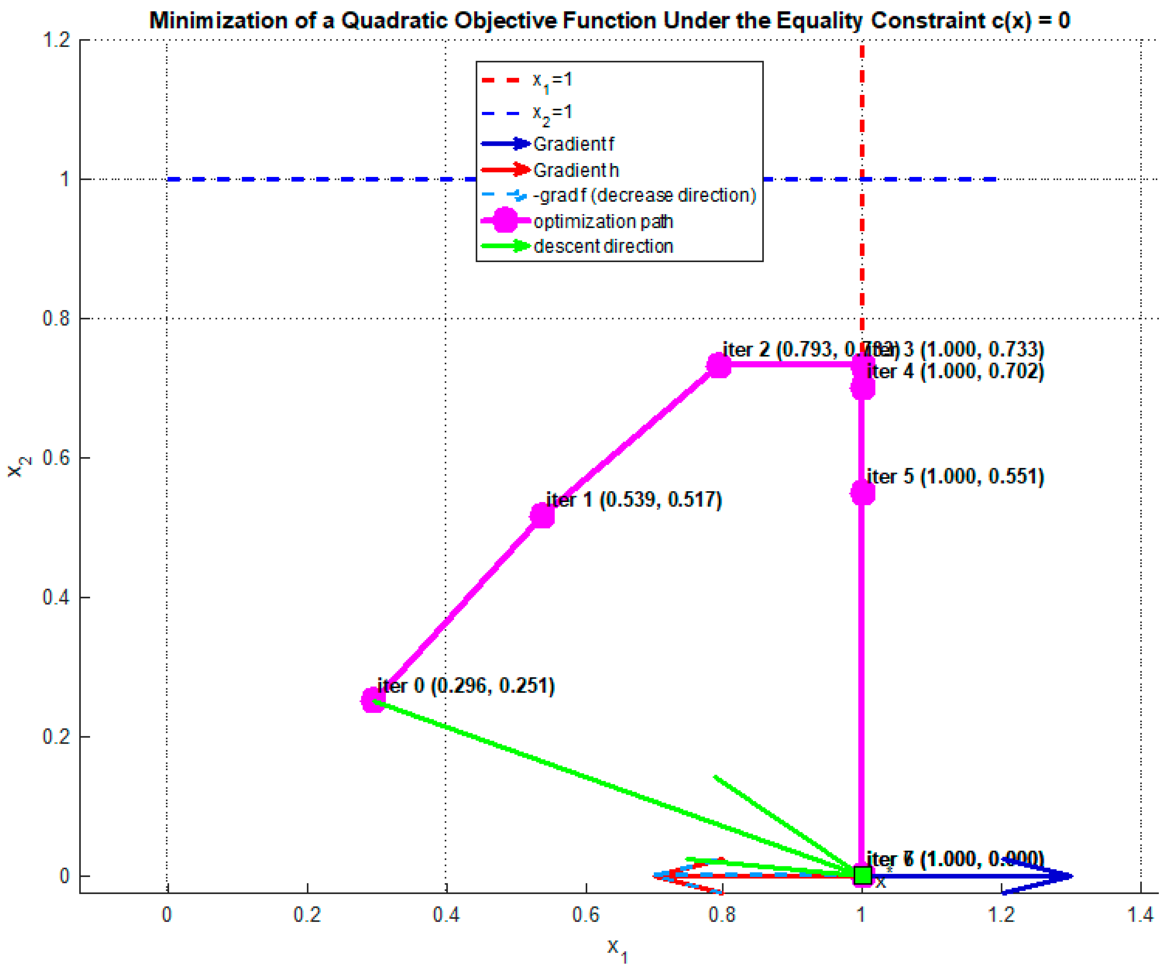
Table A2.
KKT and Checking the Second-Order Optimality Conditions.
From the optimization logs, supported by the corresponding plots, the optimality metrics were observed as follows, as also presented in [39,40,55,56,58,59,96]:
- Unique theoretical global minima: and
- The KKT conditions are fully satisfied.
- Second-order conditions (SOC): verified.
- Flat directions occur along boundaries due to zero eigenvalue.
- Visual confirmation: the two minima are unique in the feasible domain.
We noticed that the quadratic form is exactly zero. This happens because:
- One eigenvalue of the Hessian is zero, which means a flat direction.
- The tangent space at the boundary is trivial → there are no nonzero feasible directions that decrease the objective function.
The SOC is interpreted as follows:
- The zero value indicates a flat direction along the boundary.
- There is no feasible direction that can further decrease the objective.
- The SOC is technically satisfied, even though it is not strictly positive definite.
Figure A2.
Feasible Set with Unique Theoretical Global Minima and Active Constraints.
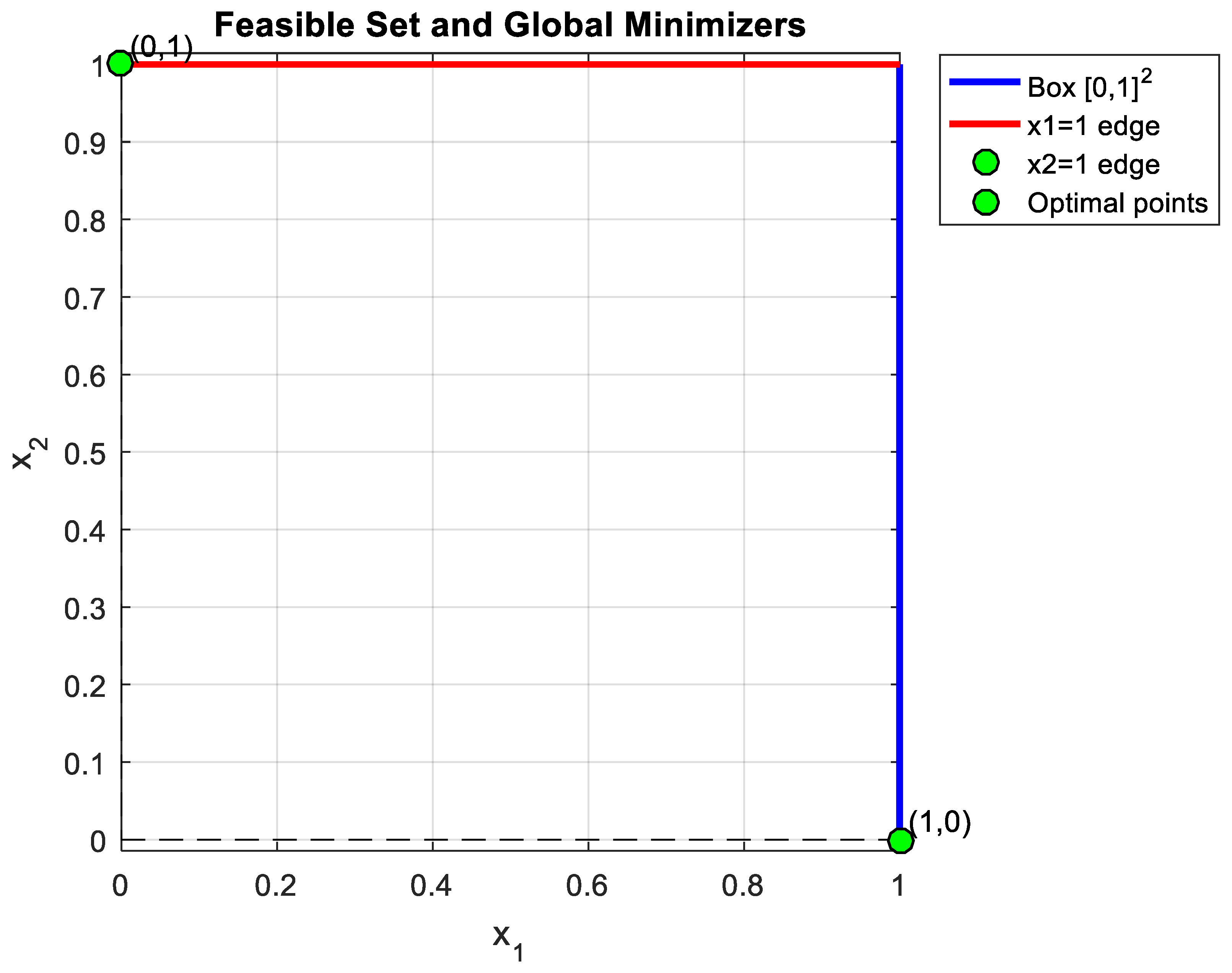
The connection with the KKT optimality conditions is as follows:
- Stationarity residual KKT stationarity is satisfied.
- Multipliers dual feasibility is satisfied.
- Primal feasibility = constraint satisfied.
- Quadratic form second-order optimality condition is satisfied.
Based on the KKT optimality condition calculations, the optimality metrics are as:
- We consider two scenarios with and without box constraints in Lagrangian Function.
- Both scenarios yield the solutions that is, and
- The box constraints defined on the decision bounds enforce boundary solutions.
- Hessian positive semi-definite along feasible directions flat direction present.
- Tangent space confirms no feasible descent direction.
- The langrage multiplier fully activates equality constraint along boundary.
Appendix B. Piecewise-Convex Feasible Region in ,
The nature of the feasible region provides the optimizer with the capability to decompose it into line segments in or convex subsets in . The solver recognizes the specific geometry and solves it efficiently. It decomposes it into a piecewise convexity model, as also evidenced in our previous studies [39,55,58,59,89,96].
This transformation permits both algorithms to navigate the search space efficiently. Then, the trajectory leads to local solutions while feasibility and optimality are met at once. A convex quadratic objective function is minimized under an equality constraint function within a box-constraint [39,40,55,56,58,59,96]:
Subject to the nonlinear constraint:
And the box constraints:
The objective function is minimized under an equality constraint with , where measures infeasibility while measures feasibility as displayed in Figure A3. The active constraint is the frontier between the infeasible and feasible region, helping us to understand the geometry of the optimization problem [58,59].
This geometry-driven optimization method allows us to find local solutions at the endpoints without relying on a non-smooth function enforcing feasibility in the case of any constraint violation. We separate the entire search space into an infeasible region that is and a feasible region . If is the active and strict equality constraint, then is indeed an infeasible region. If the inequality constraint holds true, then the feasible region is interpreted as a union of the two line segments and the interior region where and . The active constraint is the frontier between the infeasible and feasible region, helping us to understand the geometry of the optimization problem. This geometry-driven optimization method allows us to find local solutions at the endpoints. Thus, there is no need for a non-smooth function to enforce feasibility in the case of any constraint violation [96].
We separate the entire search space into an infeasible region that is and a feasible region . If is the active and strict equality constraint, then is indeed an infeasible region. If the inequality constraint holds true, then the feasible region is interpreted as a union of the two line segments and the interior region where and . Particularly, implies either:
- and and . Given ], this implies . So, this is the segment
- and . Given , this implies . So, this is the segment .
Therefore, the feasible region under is the union of the two line segments and . This region is non-convex. The main idea is to decompose the non-convex feasible region into a union of piecewise line segments in or into convex subsets in . The line segments displayed in the plot are the following as also shown in Figure A3.
Figure A3.
Nonlinear Constrained Minimization Problem in .
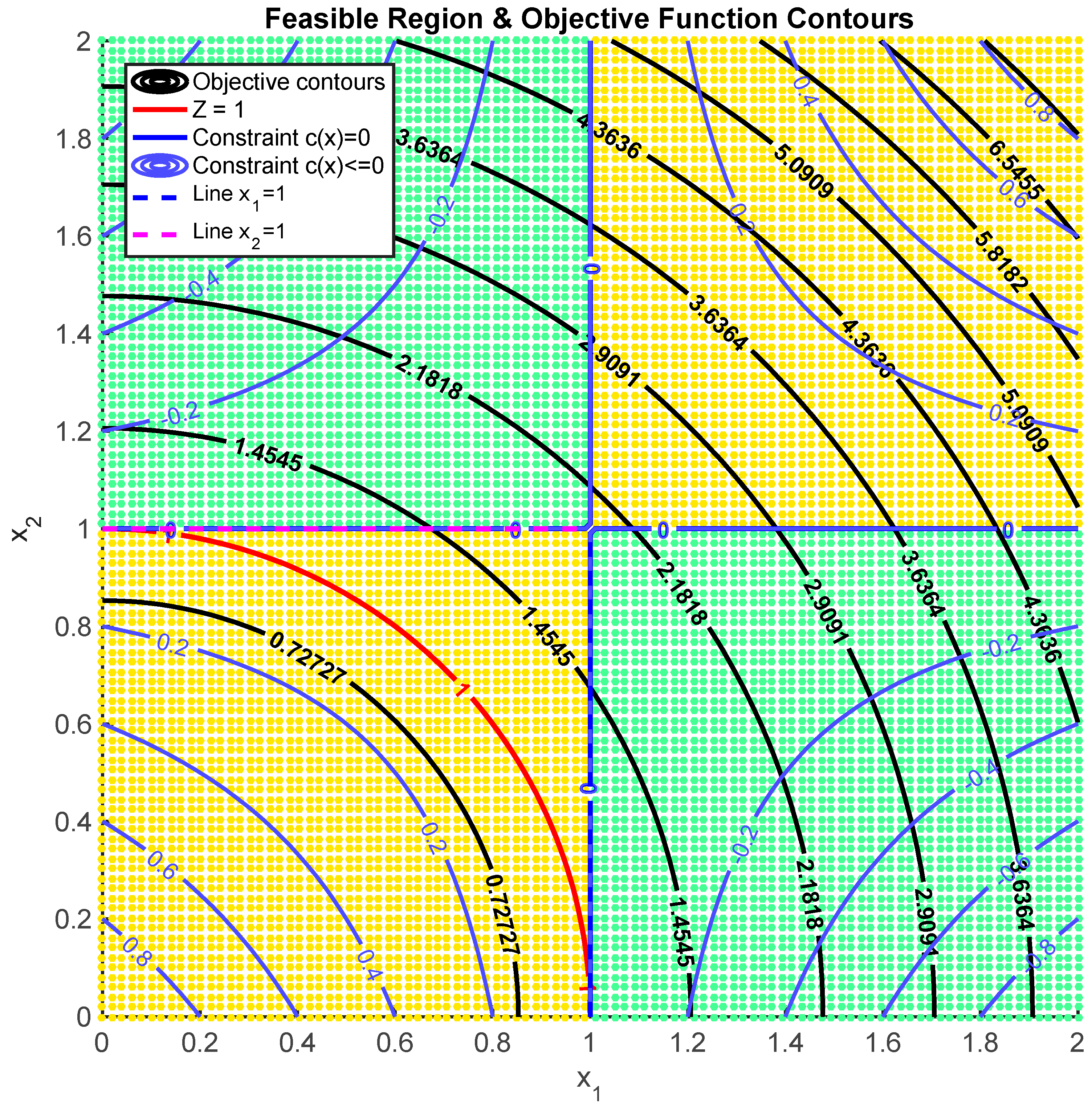
- is a convex region.
- is a convex region.
The objective function represents a paraboloid with a global minimum at the origin (0, 0), while the constraint defines a feasible region consisting of a line where either or . The feasible frontier separates the infeasible region from the feasible region (), as shown in Figure A3.
Starting from an initial point, SQP approximates a solution satisfying the KKT optimality conditions. The step length is calculated according to the Armijo condition 4, while line search computations do not prevent the step length from reaching one near the local optimum, as shown by the empirical results in [39,58,59,96].
SQP does not present a slow convergence caused by magnified second-order changes in the constraint function. SQP reaches an optimal solution upon the superlinear convergence. Thereby, the super linear convergence is preserved via a line search that decreases the non-smooth penalty function without rejecting the full step [58,59].
On the other hand, IPMs start from the interior of the feasible region, converging toward one of the line segments, achieving identical optima, with the step norm and first-order optimality approaching zero. The OPP optimization problem is declared as [33,39,54,55,58,59]:
Subject to the observability constraints [33,39,40,54,55,58,59]:
with bounds on the decision variable such as [33,39,55,58,59]:
The feasibility of the constraint can be viewed in a similar manner like the instance in . Since , each term and similarly for all neighbors . Therefore, the product is nonnegative, also proven in [59]:
The equality constraint requires that this product equals zero. However, a non-negative product equals zero only if at least one term in the product is zero, i.e.,
We conclude that the only values that satisfy the equality are as follows [39,55,58,59]:
And if none of the neighboring variables satisfies , then is forced to satisfy the equality as our foundational design presents in [59]. Otherwise, if a neighbor , is allowed. Hence, for each decision variable , the feasible values move to the extremes of the binary box-constraint, also shown in [33,39,55,58,59].
The objective function is quadratic and increasing in each , so it is minimized by taking the smallest feasible . However, the equality constraint requires at least one variable in each local neighborhood (including ) to be 1. Therefore, each can only take the binary values 0 or 1, which naturally enforces a discrete solution [59]. Therefore, the feasible set is inherently binary due to the structure of the observability constraint function combined with the box constraints, also shown in [59].
Each is found as either 0 or 1 [33]. Extending our geometric idea from and relying on geometric insight of optimal PMU placement in , we consider a piecewise-segmented convex nature of the feasible region, also shown in [59].
The feasible region has piecewise line segment structure in or segmented convex-subsets nature in due to the following algorithmic reasons.
This guarantees that a local optimization method can be executed and lead to a solution with the same quantity as the one located by a branch-and-bound algorithm in each convex region [33,39,55,58,59]. We conclude our optimality findings presented in this research work as follows:
- 1.
- Piecewise convexity model due to a union of piecewise line segments
- Each constraint can be satisfied either by or for some . Within each segment where the active variables are fixed, the feasible set for the remaining variables forms a convex subset of . This creates a piecewise-convex feasible region, where the feasible points lie at the vertices of the hypercube .
- 2.
- The piecewise convexity model is a union of convex subsets in
- The overall feasible region is a union of these convex segments corresponding to different combinations of which variables are set to 1. Because it is a union of convex sets rather than a single convex set, the overall feasible region is not globally convex, but rather piecewise convex.
- 3.
- Solving the OPP model in -Discrete boundary points at endpoints of the union of line segments and at vertices of hypercube in
- Due to the box constraints and structure of the product in the equality constraints, the feasible points collapse to the corners of these convex segments, i.e., or . This is why the solution is naturally binary [33,39,55,58,59].
- 4.
- Quadratic objective function
- The objective is strictly increasing in each . Therefore, the solver prefers to minimize the sum of squares, which pushes most variables to 0, while still satisfying the equality constraints (forcing some to satisfy observability 59).
- 5.
- Optimizer Solver Behavior in Solving the OPP model
- SQP or IPM solvers starting from an arbitrary starting point converge to boundary solutions or .
- Multi-start initialization may land in different degenerate convex segments, but within each, the solution behaves as a convex NLP model.
- The Maratos effect is avoided, which means that the full step lengths are accepted, feasible iterates are generated, and therefore, the constraints remain feasible.
- Finally, a local minimum with global-like characteristics is achieved with the convergence to be superlinear.
- 6.
- Significance of the mathematical structure of the optimization model.
We minimize a quadratic objective function subject to polynomial function that leads into a piecewise convexity model. The structure of the optimization problem is not a pure non-convex model, even though it belongs to nonlinear non-convex programming [1,2,3,4,5,6,7,8]. The binary structure and piecewise nature induce degenerate convex subregions [33,39,55,58,59].
This justifies why continuous NLP formulations give the same binary solution as the classical ILP, even for large-scale networks (e.g., 2383-bus Polish grids in MATPOWER) [92,93]. The global optimality is achieved without direct comparison to ILP model solutions [33,39,55,58,59]. In the OPP problem in , the solution is located at the boundaries (). The SQP step length remains full, that means, as shown in the optimization logs and figures. The decision variables converge to or due to the following optimality quantities being produced in the iterative scheme [33,39,55,58,59].
- Equality constraints are satisfied by setting at least one term of the product to 0 ( for coverage and an accurate state estimation process [33,39,55,58,59]).
- The objective is minimized by pushing all other variables to 0 [58,59].
Even though the NLP formulation has products with a non-convexity structure, it is degenerated locally into convex regions corresponding to different binary assignments.
The feasible region is the union of these segments, forming a piecewise-convex or segmented convex) region. Therefore, the optimizer solves effectively convex subproblems, leading to exact binary solutions [33,39,40,55,58,59]. Each convex segment corresponds to a particular pattern of active variables . The quadratic objective function is increasing in each , so the optimizer selects the lowest feasible values, constrained by the segments, resulting in binary solutions, as shown in [33,39,55,58,59].
Appendix C. Iteration Logs and Convergence Analysis
In geometric optimization, the underlying structure or geometry of the feasible region is decomposed into a union of piecewise line segments in or convex subsets in , guiding the iterative algorithm’s trajectory toward optimality [39,40,55,58,59].
From a theoretical perspective, the piecewise convexity model acts as a local convexification of the entire feasible region. By adopting local convexification, the Maratos effect, which occurs in SQP methods, is effectively avoided. Numerical results show that the local quadratic model accurately represents the curvature of both the objective and constraint functions within each sub-region. The convex partitioning prevents curvature mismatches and instabilities near constraint intersections [59,74,75,76,77,78,79,80,81,82,83,84,85,86,87,88].
Using the local convex geometry of this region, SQP methods linearize the constraints while preserving second-order curvature information [39,40,55,58,59]. This allows SQP methods to take full steps without violating the constraint function. In contrast, IPMs embedded in Fmincon and Ipopt solvers preserve feasibility through barrier terms that keep the iterations within the interior of this feasible region [89,90,91]. The feasible region is piecewise convex, a union of convex segments with endpoints at 0 and 1 [39,55,58,59].
SQP and IPMs handle equality constraints, maintaining both feasibility and optimality simultaneously [39,55,58,59]. The solver then moves smoothly along search directions without step reductions or erratic behavior [39,40,55,58,59].
The logs and plots show that SQP methods start from an infeasible point and quickly enter one of the convex line segments (e.g., ). Full step lengths are consistently taken once feasibility is achieved. Both norm of step and first-order optimality norm approach zero, and there is no violation in the constraint function.
On the other hand, IPMs move from the interior of the feasible region, satisfying the barrier terms, and finally deliver local solutions with binary-valued nature [39,55,58,59].
The objective function monotonically decreases along the piecewise-convex segment, reaching 1.0 at its final value. The constraint function is given as: .
The piecewise convex nature of the inequality constraint ensures that once captured, the optimizer remains within a specific line segment. Once Fmincon and Ipopt capture the piecewise line segment or , the constraint function is fully satisfied, and the objective function is minimized until the optimal value of 1.0 has been reached. The piecewise convex optimization enables SQP and IPMs to preserve superlinear convergence characteristics, also proven in [33,39,40,55,58,59,96].
Initial and final points are displayed along with the union of line segments and parabolic curves due to the bilinear term . SQP proceeds directly toward one of them.
IPMs start from the interior and converge to the same piecewise line segment [39,55,58,59]. Both algorithms find local solutions at the endpoints of the union of line segments.
This geometric approach guarantees feasibility without the need for non-smooth penalty functions 59. Thus, the trajectory naturally moves to one of the piecewise line segments and converges to a feasible endpoint— or —where attains its minimum. Starting from different initial points, iterative algorithm trajectories consistently progress toward a piecewise line segment, with constraint violation decreasing rapidly to zero. The SQP and IPMs then move along that segment and converge to a solution located at the boundaries of }. The norm of step initially steadily decreased to zero, while the first-order optimality norm approaches zero as the process converges. These optimality metrics confirm that local convexification helps avoid the Maratos effect [74]. As a result, its negative impact on the preservation of the superlinear convergence rate and the quality of the solution are avoided, as also demonstrated in our previous works [39,40,58,59].
Plots and Figures Explanations
The proposed piecewise convex decomposition allows the optimizer solvers to maintain feasibility and optimality simultaneously throughout the iterative process, eliminating the need for non-smooth penalty functions, filters, or watchdog correction techniques. The primary innovation of this work lies in the geometry-driven approach to non-convex optimization. By decomposing the non-convex feasible region into line segments in , the methodology enables SQP and IPMs to navigate the search space while preserving superlinear convergence near local optimum [33,39,40,55,58,59,96].
The algorithms leverage local convexification to navigate efficiently along feasible segments and reach binary solutions, as shown by the empirical results in [39,40,55,58,59].
Moreover, the geometric decomposition eliminates oscillations and non-monotone zig-zag trajectories, enabling SQP and IPMs to detect local optima located at the endpoints of the piecewise line segments. Both the norm of step and first-order optimality approach zero at convergence. Regardless of the starting point, SQP and IPMs consistently converge to the same binary local solution due to the piecewise convexity of the feasible region [96].
SQP and IPMs produce binary solutions due to the multiple-choice constraints, aligning continuous optimization with combinatorial outcomes [39,40,58,59]. These solutions exhibit global-like characteristics, satisfying KKT conditions while adhering to multiple-choice constraints. Multiple initial points were tested to confirm this behavior [96].
Multiple trajectory plots demonstrate that the convergence behavior is systematic rather than coincidental [59]. These plots illustrate how both SQP and IPMs guide their trajectory toward one of the line segments, move along it, and converge to a solution at the boundaries. The analysis of optimization logs and numerical results confirms the following convergence and optimality metrics, as also demonstrated in [33,39,40,55,58,59,96]:
- Full steps are taken once feasibility is satisfied.
- Constraint violations decrease smoothly to zero.
- The objective function reduces monotonically to its optimal value .
- First-order optimality and norm of step approach zero without oscillation.
- Superlinear or quadratic convergence is achieved in later iterations.
Each plot corresponds to a different starting point, showing that both SQP and Ipopt navigate toward the feasible boundary and converge to local optima [59], i.e., . Across multiple initializations, SQP consistently accepts full steps after early iterations. It achieves feasibility within two to three iterations as shown in the logs with the plots. The objective function, norm of step, and first-order optimality decrease smoothly without oscillation. Fmincon did not take any damped steps near the solution, as also evidenced by our previous works [39,55,58,59,96].
These convergence metrics confirm that the Maratos effect does not occur. In this context, the line search and non-smooth penalty function do not reject the full Newton step [96]. This geometry-based optimization approach is validated through optimizer logs. Multiple initial points are selected, while convergence to boundary solutions is consistent and independent of the starting point. By taking full step-lengths during line search computations, the Maratos effect is avoided, ensuring superlinear convergence [39,58,59].
Consequently, the SQP algorithm exhibits superlinear convergence toward the constrained local minima, as shown in Table A3. The Fmincon logs show that the SQP iterates directly toward one of the piecewise line segments, partially exploring the feasible region.
Once the algorithm captures one of the line segments, it moves along that segment toward optimality. Therefore, zig-zag oscillations between the line segments are avoided and converge smoothly to the endpoints (1, 0) or (0, 1). It emphasizes the trajectory behavior along the piecewise-convex line segments, which is critical to understanding the convergence and the avoidance of the Maratos effect [74].
The SQP takes full steps in the line search with good computation in the trust region. These quantities indicate that the local geometry of the region actively contributes to avoid the Maratos effect [74]. The objective function decreases monotonic toward its optimal value. A local minimum is reached, based on the fact that both first-order optimality and the norm of the last displacement, approach zero [39,40,58,59,96].
The optimizer navigates within these convex segments until it reaches a boundary . As observed in Table A3, the objective function initially increases monotonically from iteration 0 to iteration 3. From iteration 4 to iteration 7, the objective function smoothly decreases, reaching its optimal value of 1 [33,39,40,55,58,59,96].
Once the Fmincon captures , the feasibility remains zero until the final iteration. Therefore, the SQP produces feasible iterates from iteration 3 toward 7. Both norm of the step and first-order optimality decrease smoothly and monotonically. This confirms a stable convergence with the absence of oscillatory behavior [33,39,40,55,58,59,96].
Thereby, the Maratos effect is avoided due to the piecewise convexity approach, without needing a non-smooth penalty function to fix infeasibility. The Fmincon optimizes the nonlinear model with smooth convergence and monotonic behavior toward a local solution located at the endpoint , without needing corrective measures due to any constraint violation as shown in Table A3 and Table A4. The optimization logs also confirm that the Maratos effect is avoided [74]. Therefore, there is no need for penalty functions, filter methods, or step truncation for maintaining feasibility [3,4,33,39,40,55,58,59,96].
Table A3.
SQP embedded in Fmincon Solver Iteration Logs toward optimality.
Table A4.
Fmincon solver results, based on the optimization logs, are presented in Table A3.
This behavior preserves the superlinear convergence rate near the solution [33,39,58,59]. As observed, both feasibility and optimality are satisfied simultaneously at each iteration once the algorithm captures one of the line segments, also proven in [39,55,58,59].
Fmincon exploits the geometry of the feasible region and interprets it as a union of piecewise-linear or piecewise-convex segments [33,39,55,58,59]. This decomposition allows the SQP to maintain feasibility while the trajectory moves along one of the line segments toward the endpoints or . The SQP trajectory reaches , avoiding the Maratos effect [74], without requiring non-smooth penalty functions, second-order corrections, or watchdog methods, as shown in Figure A4.
Figure A4.
Fmincon iterative trajectory toward feasibility and optimality.
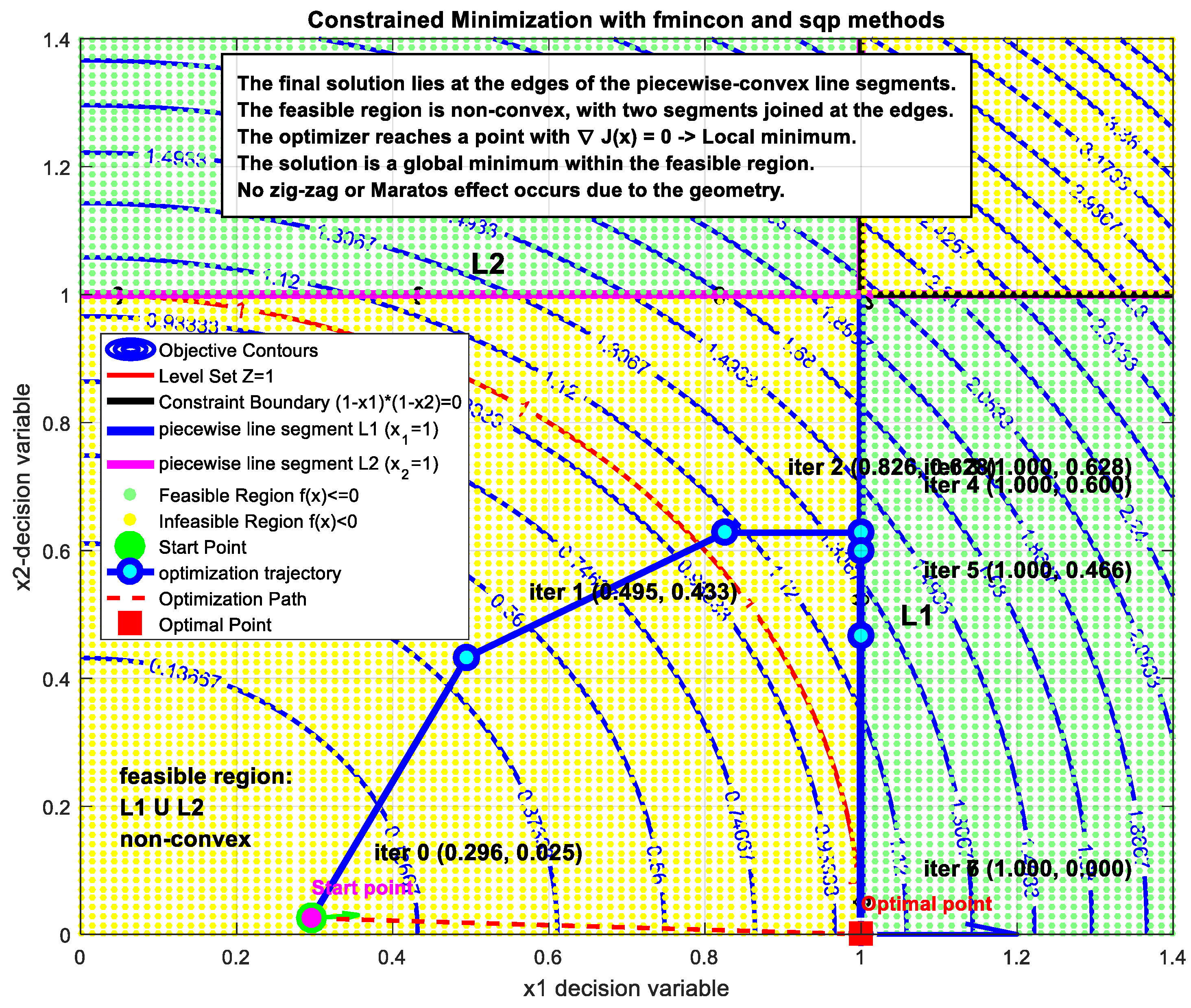
Additionally, the objective function decreases smoothly to its optimal value (e.g., ). Although the nonlinear model has a non-convex structure, the Fmincon obtains non-strict global solutions at the endpoints of the union: . As shown in Figure A4, the optimality metrics are as follows:
- Green point: Starting point (infeasible).
- Red point: Final solution —on the convex line segment x1 = 1.
- Blue line: Feasible region .
- Red line: Feasible region .
- Optimization trajectory: SQP iteration path, showing rapid entry into the convex sub-hull and smooth descent along the line segment.
The analysis of the iteration log is shown in Table A3, followed by Table A4. We highlight smooth convergence toward optimality. As observed from the optimization log, we summarize the optimality and convergence metrics as follows [39,40,55,58,59,96].
- The SQP algorithm starts from an initial point within the infeasible region , where the constraints are violated, and feasibility is nonzero.
- The line search calculates directions and allows full steps, ensuring smooth progress toward optimality.
- Once the SQP algorithm captures one of the line segments, constraint feasibility reaches zero.
- The SQP algorithm moves smoothly toward a solution at the endpoints of the union, enabling superlinear convergence. In this context, the solution remains at the endpoints of the piecewise convex line segment.
- A unity step is taken, and the step norm and first-order optimality approach zero, indicating that the SQP method reaches a local optimum.
- The objective function value decreases toward 1.0, with monotonic convergence.
- The local optima lie at the endpoints of the union of the lines and .
- The local optima are also global optima because the objective function is convex within the locally convex regions.
Fmincon successfully solved the nonlinear minimization model, returning an optimal solution as shown in Table A5. For the nonlinear problem in , the feasible region is a union of piecewise line segments. Fmincon guides its trajectory toward one of the line segments while an optimal solution is achieved, as shown in Figure A5. SQP exhibits smooth and monotonic convergence toward the optimal solution at .
From iteration 5 onward, the objective function steadily decreases to its optimal value of 1, with zero constraint violation. Both the step norm and first-order optimality decrease smoothly, confirming stable convergence and the avoidance of oscillatory behavior. Feasibility is maintained through the feasible iterates, with the SQP algorithm demonstrating superlinear convergence as it approaches the optimal solution of 1.0. This confirms that the Maratos effect is avoided [74], and no non-smooth penalty functions or corrective measures are needed [39,40,55,58,59,96].
Table A5.
SQP embedded in Fmincon Solver Iteration Logs toward optimality.
The search direction and the trust-region or line-search calculations result in effective steps. SQP converges smoothly to the local optimum, with an objective function value of 1.0. Feasibility and optimality are achieved simultaneously, as shown in Table 5 [3].
Consequently, the Maratos effect is avoided due to the piecewise convexity, without the need for a non-smooth penalty function to enforce feasibility, and the first-order optimality measure reaches zero [39,40,55,58,59,96].
Figure A5.
Fmincon iterative trajectory toward feasibility and optimality.
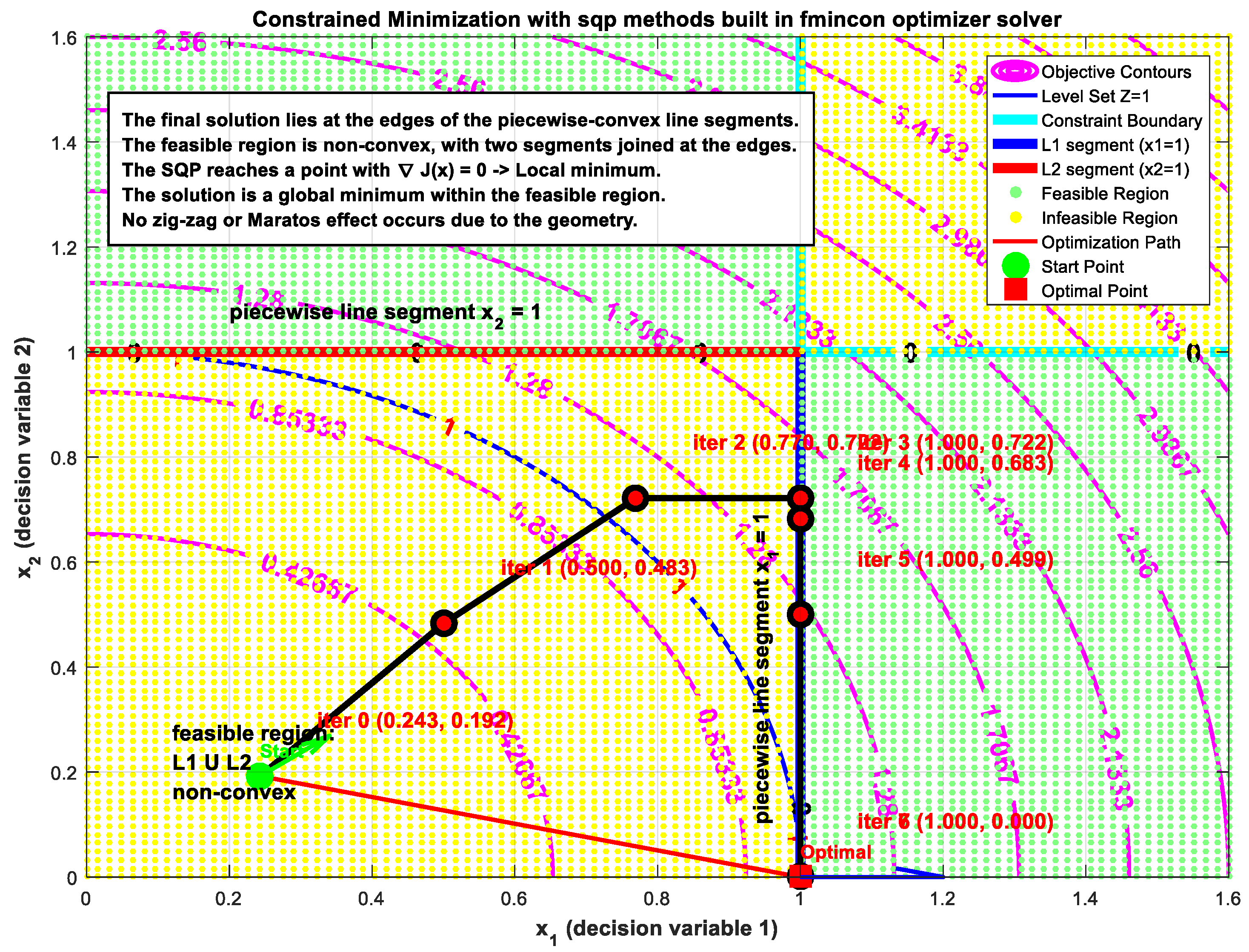
IPOPT is a primal-dual interior-point method based on a line search filter strategy to find a local solution of the nonlinear model without taking into account the decision bound [39,58,59]. Starting from (), Ipopt converged in 10 iterations to the optimal solution () with an objective function ) [4,5].
Once Ipopt captures a line segment, it progresses along it, taking full steps in the trust-region line search. Ipopt converges to a local minimum, with zero constraint violation, negligible NLP error. The KKT conditions are fully satisfied, consistent with the empirical results in [39,55,58,59,96]. The equality constraint is satisfied exactly. This means that the Interior Point NL solver terminated the iterations with both primal and dual infeasibility ≈ 0 as shown in Table A6 [4,6,90].
As observed in the optimization log and in Figure A6, the Ipopt iterates converge smoothly to the local minimum at () with an objective function value of 1.0. The primal and dual residuals decrease steadily throughout the iterations, while the barrier parameter is effectively managed, confirming robust interior-point progress, also proven in [39,40,55,58,59,96]. The objective function decreases monotonically toward its optimal value, reaching the local minimum, as shown in Figure A6 [39,40,55,58,59,96].
Constraint violations and complementarity are zero, and the dual infeasibility reaches MATLAB precision. Both primal and dual optimality conditions are satisfied. Overall, the iterates follow the feasible line segment directly toward the solution, demonstrating that a local minimum is achieved [59]. IPMs are embedded in fmincon and successfully solved the minimization problem, as shown in Table A7. Starting from , the solver converged in 9 iterations to the solution along with , without any constraint violation [39]. The objective function is non-decreasing in all feasible directions, indicating convergence to a feasible local minimum [39,40,55,58,59,96].
No feasible direction can further decrease the function’s value, and all constraints remain satisfied, as shown in Figure A7. Thus, the algorithm has reached a point where improvements are no longer possible within the given tolerances [89,90,91].
Both first-order optimality and the norm of the step approached zero within the predefined tolerances. This implies that the gradient of the objective function forms a non-acute angle with all feasible directions. Consequently, the KKT conditions are satisfied, ensuring both stationarity and feasibility at the solution [33,39,40,55,58,59,96].
Table A6.
IPMs embedded in IPOPT Solver Iteration Logs toward optimality.
Figure A6.
Ιopt iterative trajectory toward feasibility and optimality.
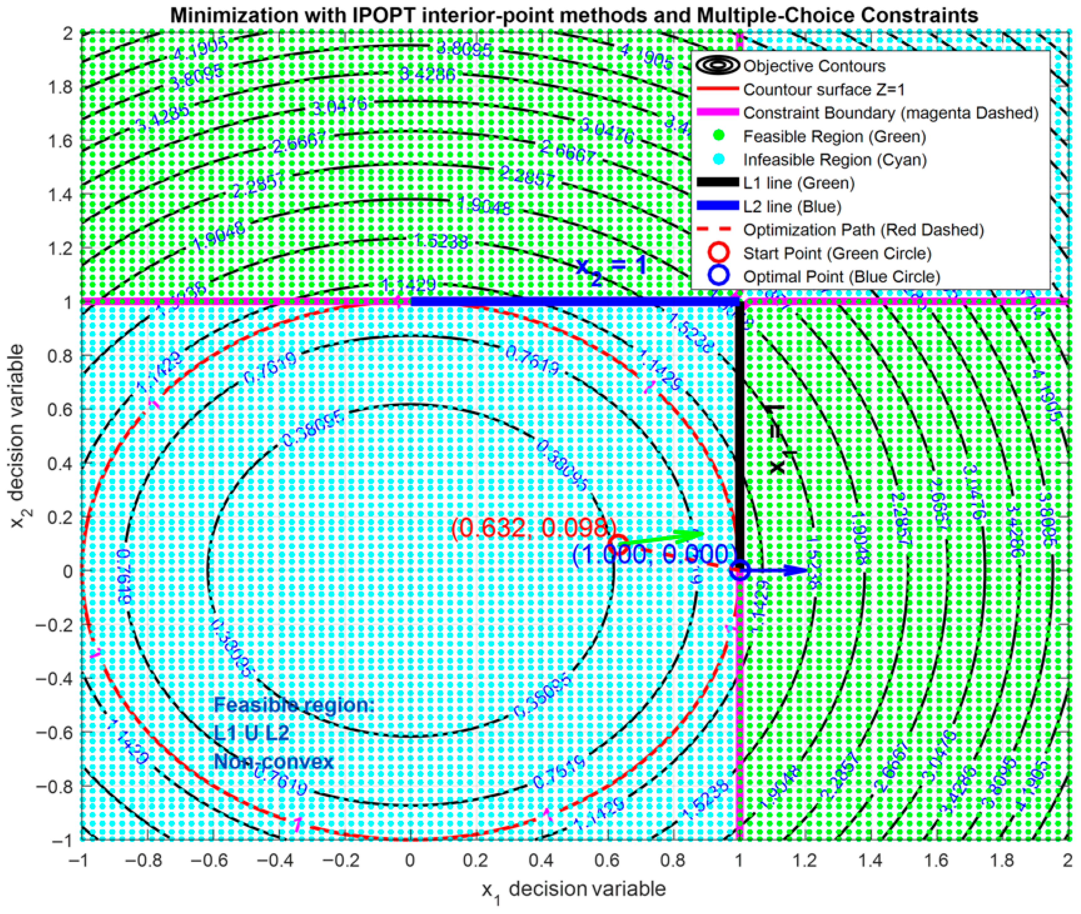
Table A7.
IPMs embedded in Fmincon Solver Iteration Logs toward optimality.
Figure A7.
Fmincon iterative trajectory toward feasibility and optimality.
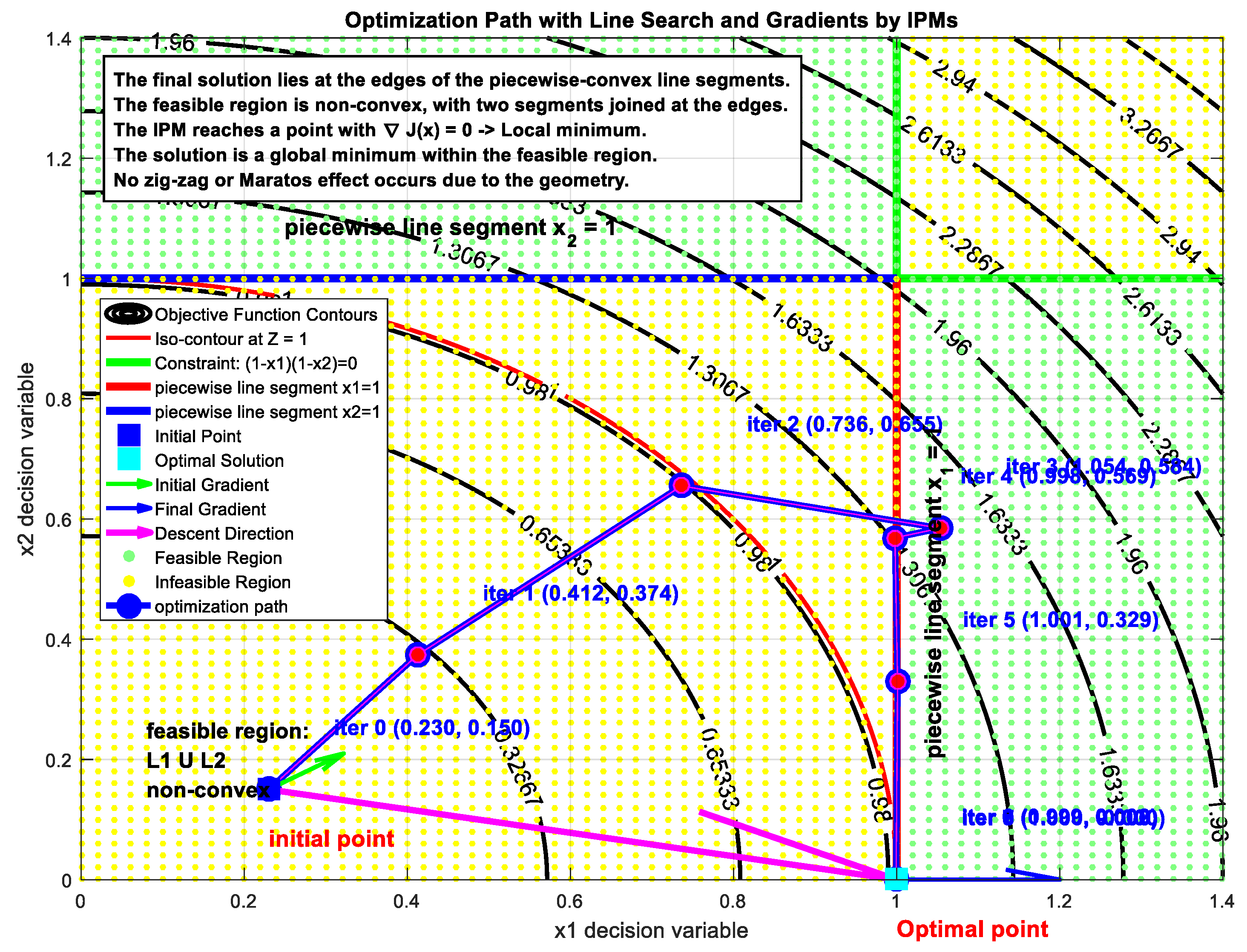
Multiple initializations confirm that the piecewise-convexity approach inherently avoids the Maratos effect [39,55,58,59,74]. This further supports the fact that the local geometry efficiently guides the iterative algorithm’s trajectory toward the local minimum. This performance is not solver-specific [59]. It is an intrinsic feature of the algorithms when handling the piecewise-convex feasible region in order to reach a feasible and local optimum. Fmincon keeps the descent direction toward the best local optimum, while Ipopt follows a smooth primal–dual path that consistently leads to the same optimum, as also proven in optimization logs [39,40,58,59]. Fmincon and Ipopt satisfy the polynomial constraint of the minimization problem. SQP and IPM trajectories converge smoothly and consistently to one of the line segments, locating the local minima at their endpoints [59]. Once the optimizer identifies a line segment or , it progresses along it and ultimately reaches the solution at the endpoints: and .
As observed in the plot and shown in Figure A8, Figure A9, Figure A10, Figure A11, Figure A12, Figure A13, Figure A14, Figure A15, Figure A16, Figure A17, Figure A18, Figure A19, Figure A20, Figure A21, Figure A22, Figure A23, Figure A24 and Figure A25, the objective function exhibits strictly monotonic improvement toward its optimal value [39,40,55,58,59,96].
Figure A8.
Fmincon iterative trajectory toward feasibility and optimality.
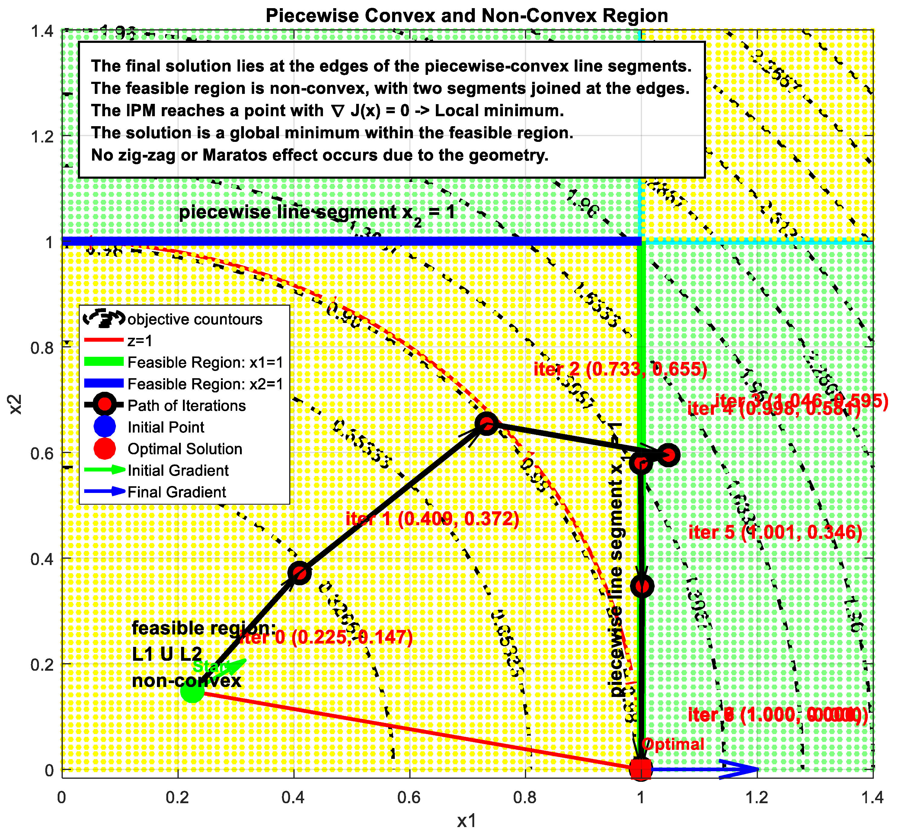
Figure A9.
Fmincon iterative trajectory toward feasibility and optimality.
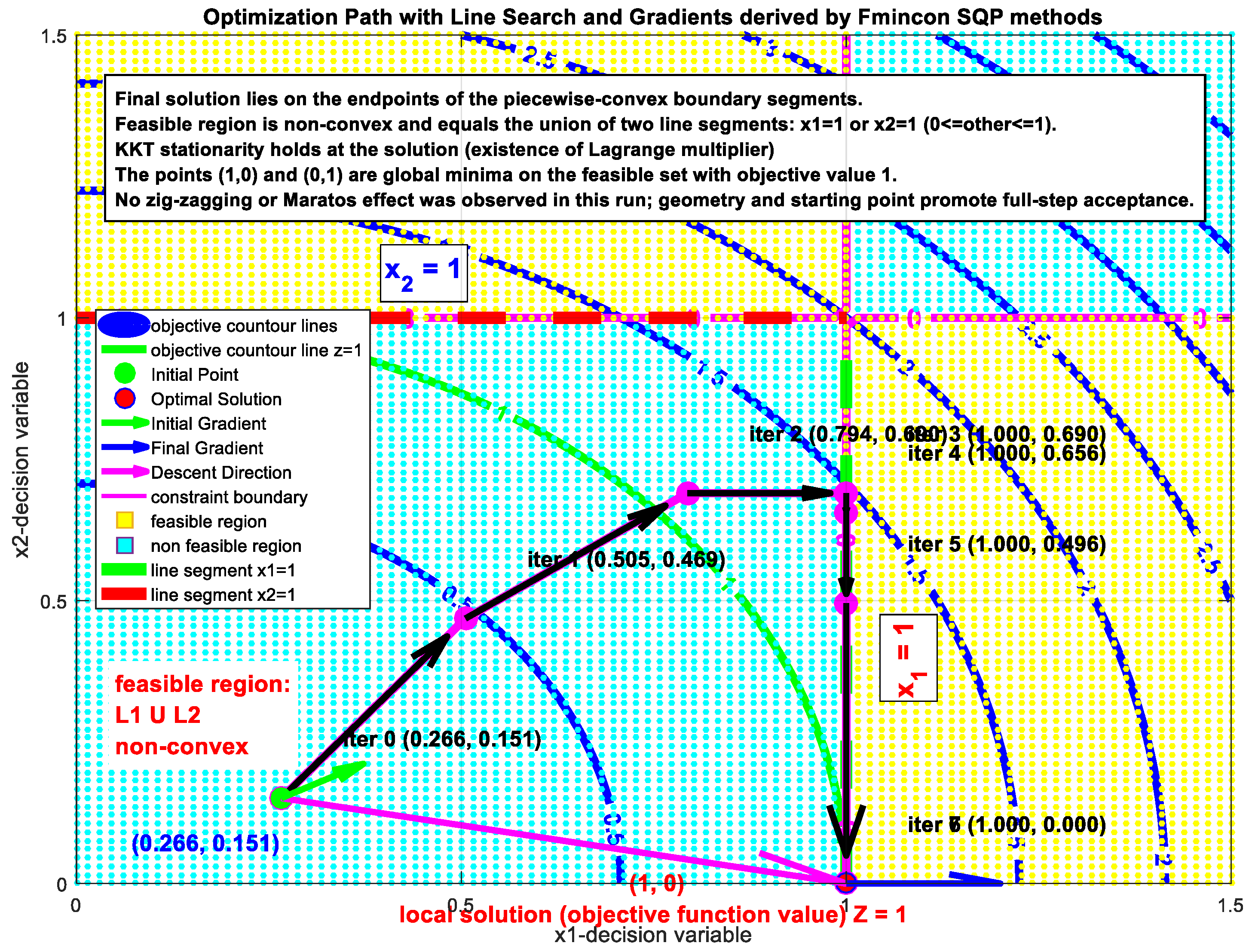
Figure A10.
Fmincon iterative trajectory toward feasibility and optimality.
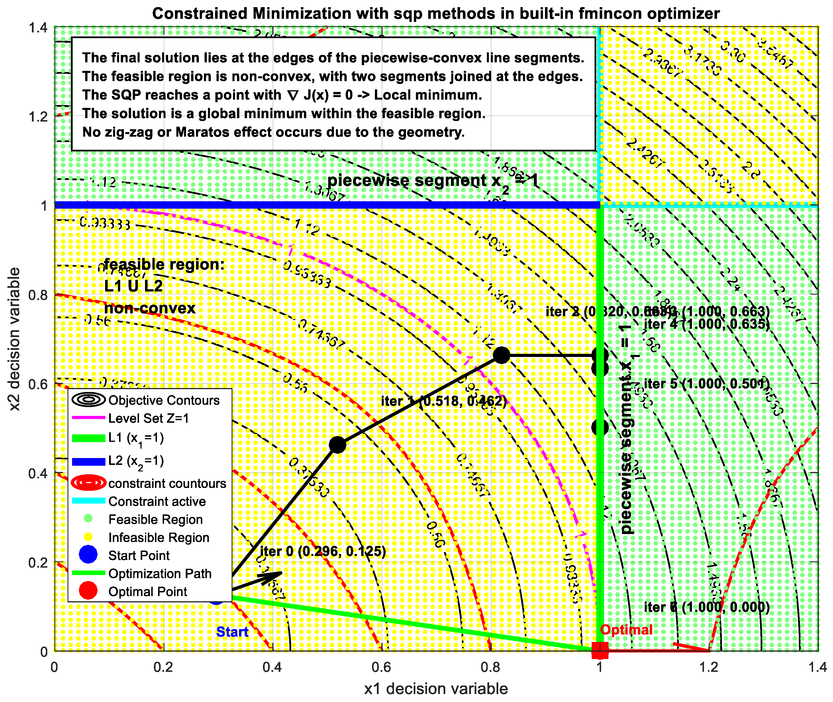
Figure A11.
Fmincon iterative trajectory toward feasibility and optimality.
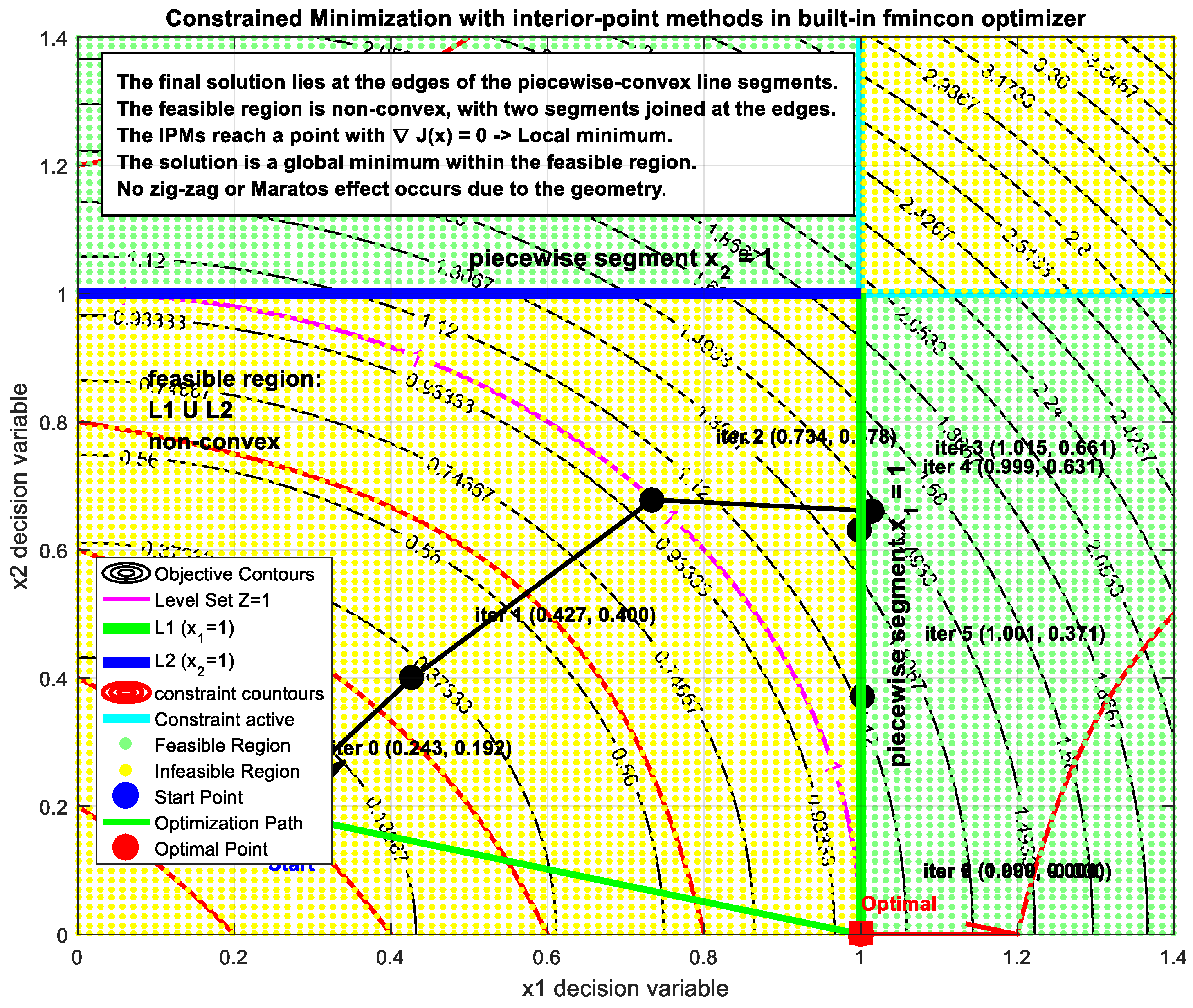
Figure A12.
Fmincon iterative trajectory toward feasibility and optimality.
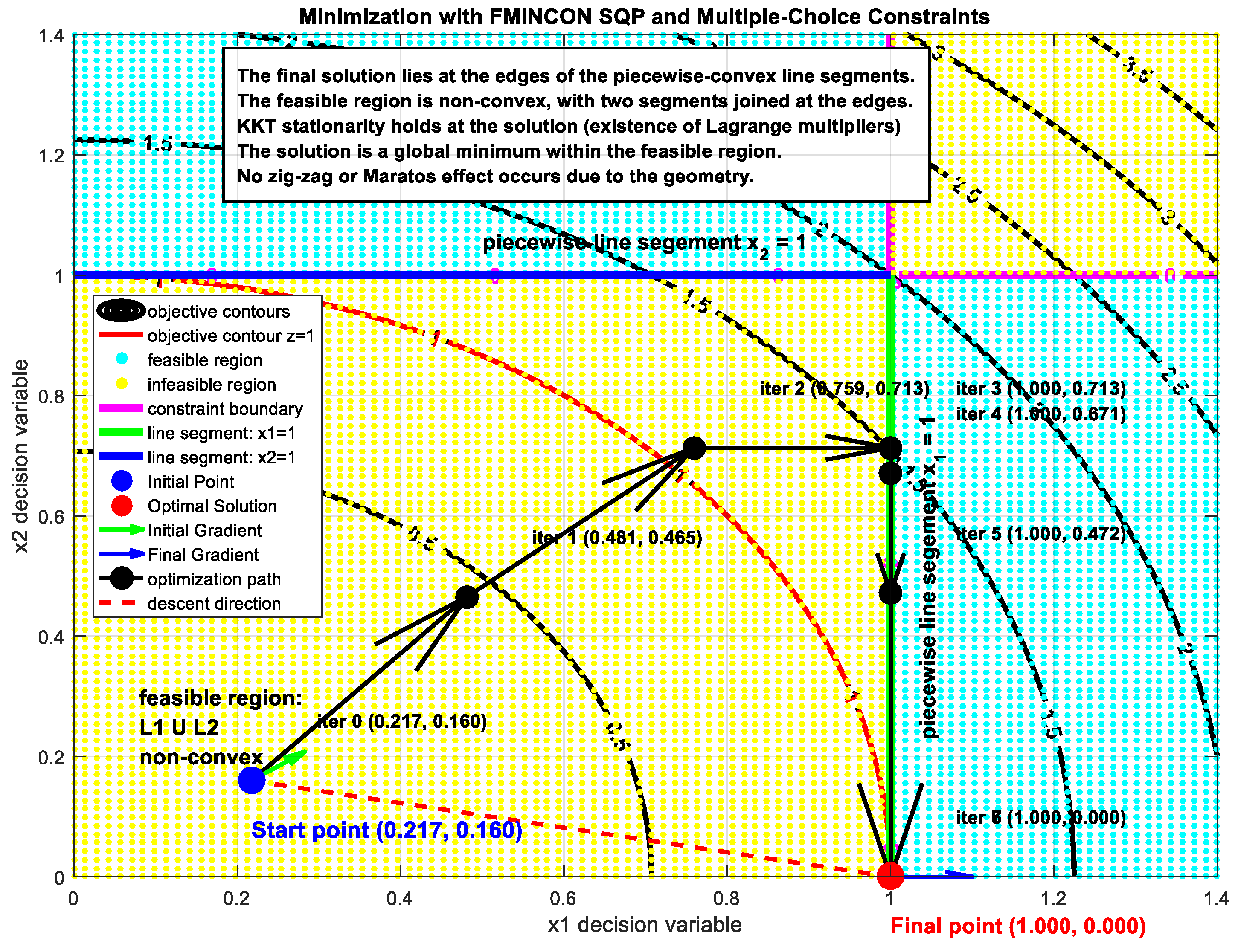
Figure A13.
Fmincon iterative trajectory toward feasibility and optimality.
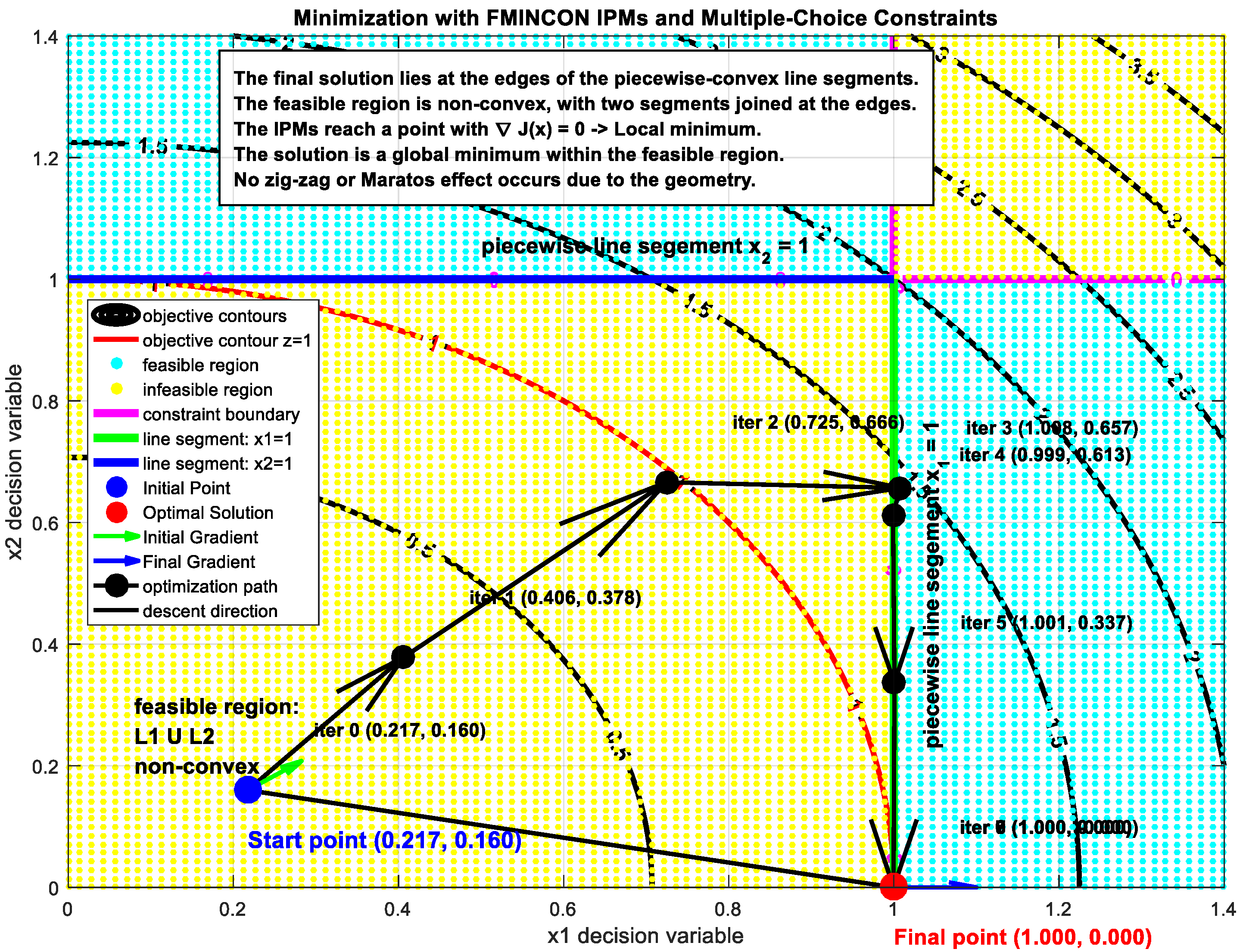
All executions start from a random initial point. The iterative trajectory moves to one of the line segments, and once the line segment is captured, feasibility is satisfied [3].
Fmincon and Ipopt are performed in MATLAB, as shown in the optimization logs and in Figure A8, Figure A9, Figure A10, Figure A11, Figure A12, Figure A13, Figure A14, Figure A15, Figure A16, Figure A17, Figure A18, Figure A19, Figure A20, Figure A21, Figure A22, Figure A23, Figure A24 and Figure A25 included in this appendix. The objective function is then monotonically minimized to its optimal value of 1. SQP keeps the descent direction toward the local optimum located at the endpoints, namely, and . Ipopt follows a smooth primal–dual path that consistently leads to the same optimum. This smooth behavior is confirmed by multiple initializations [58,59,96].
Figure A14.
SQP and IPMs iterative trajectory toward feasibility and optimality.
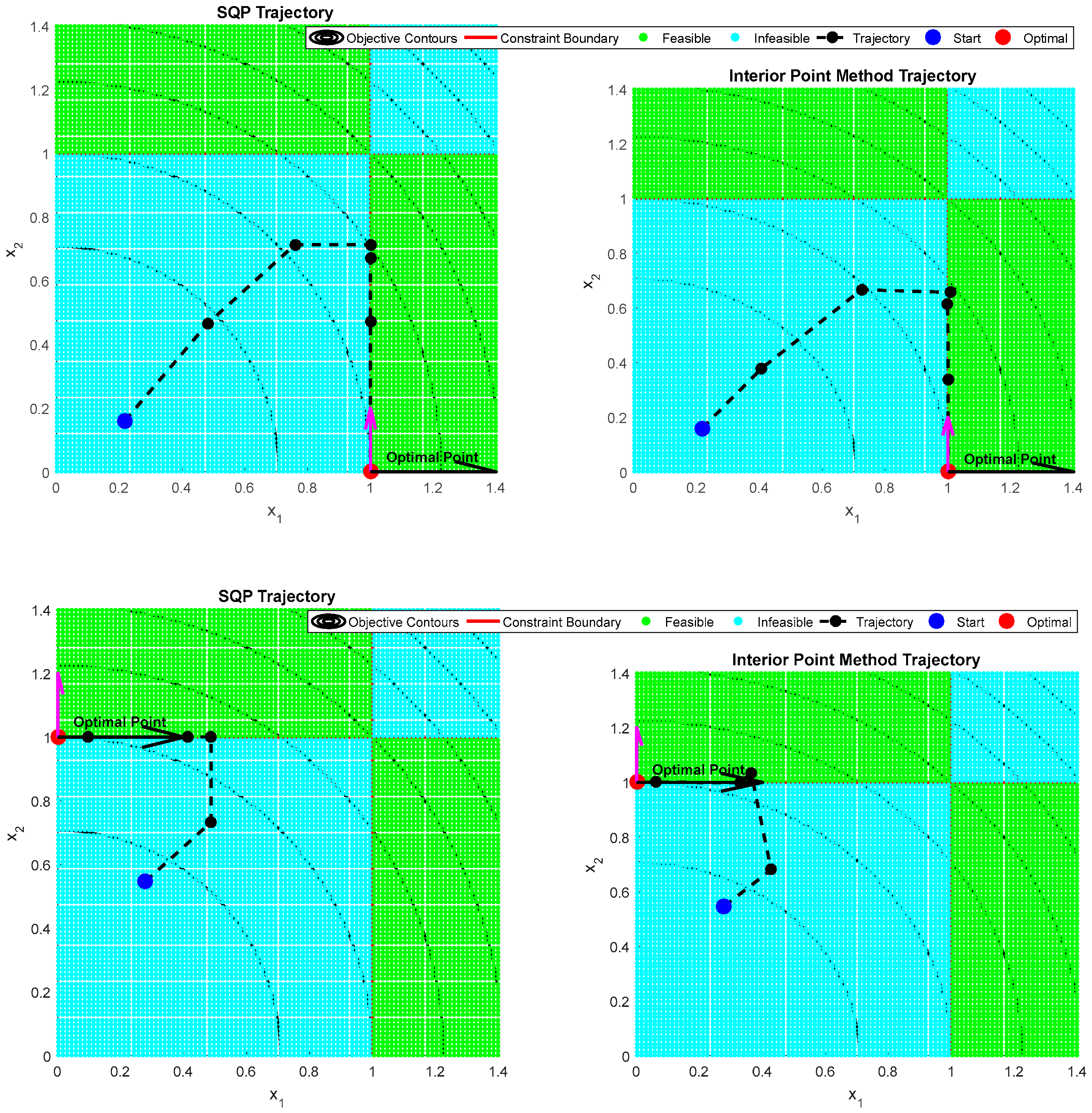
Figure A15.
Fmincon iterative trajectory toward feasibility and optimality.
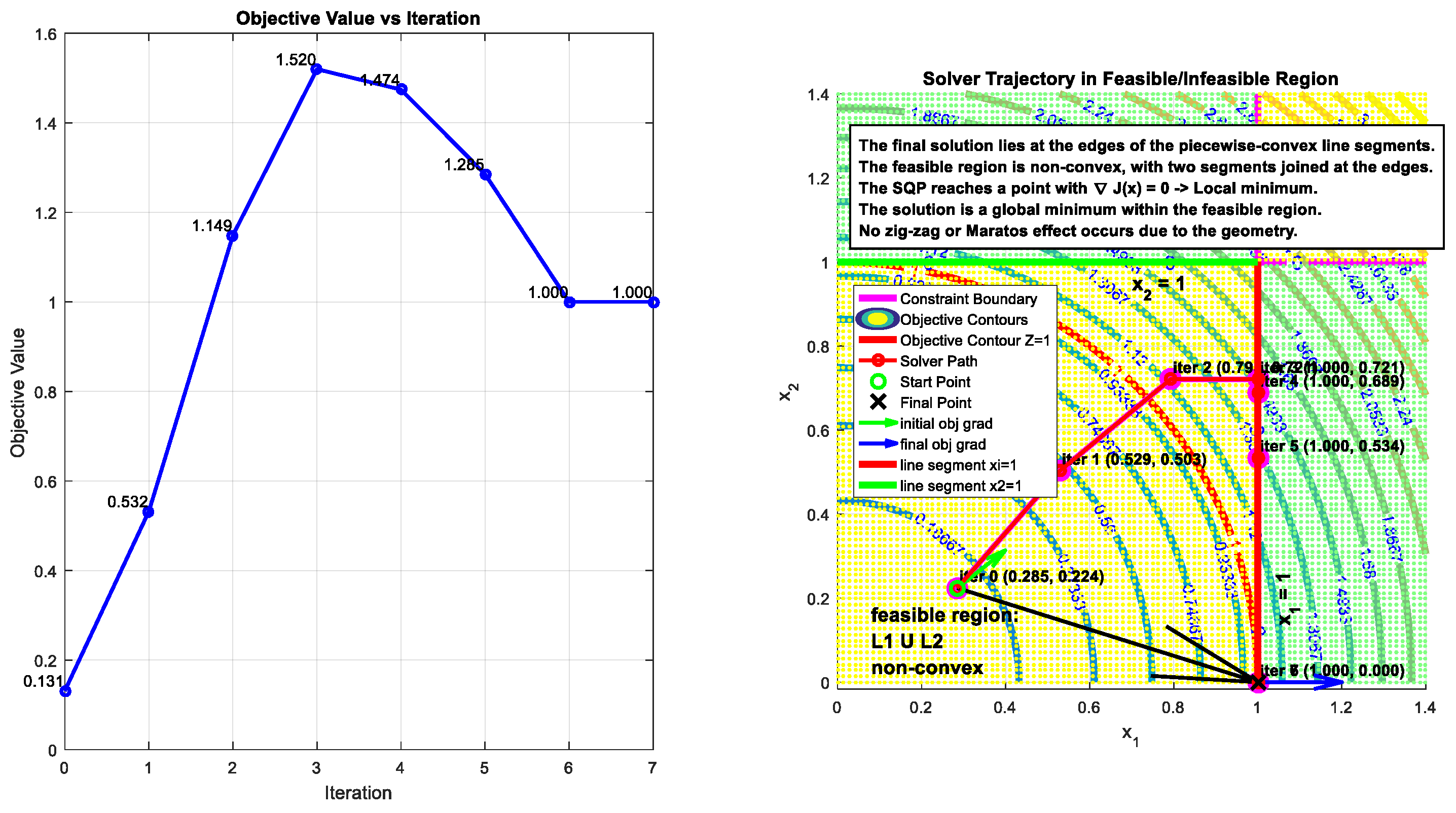
Figure A16.
Iterative monotic trajectory satisfying feasibility and optimality.
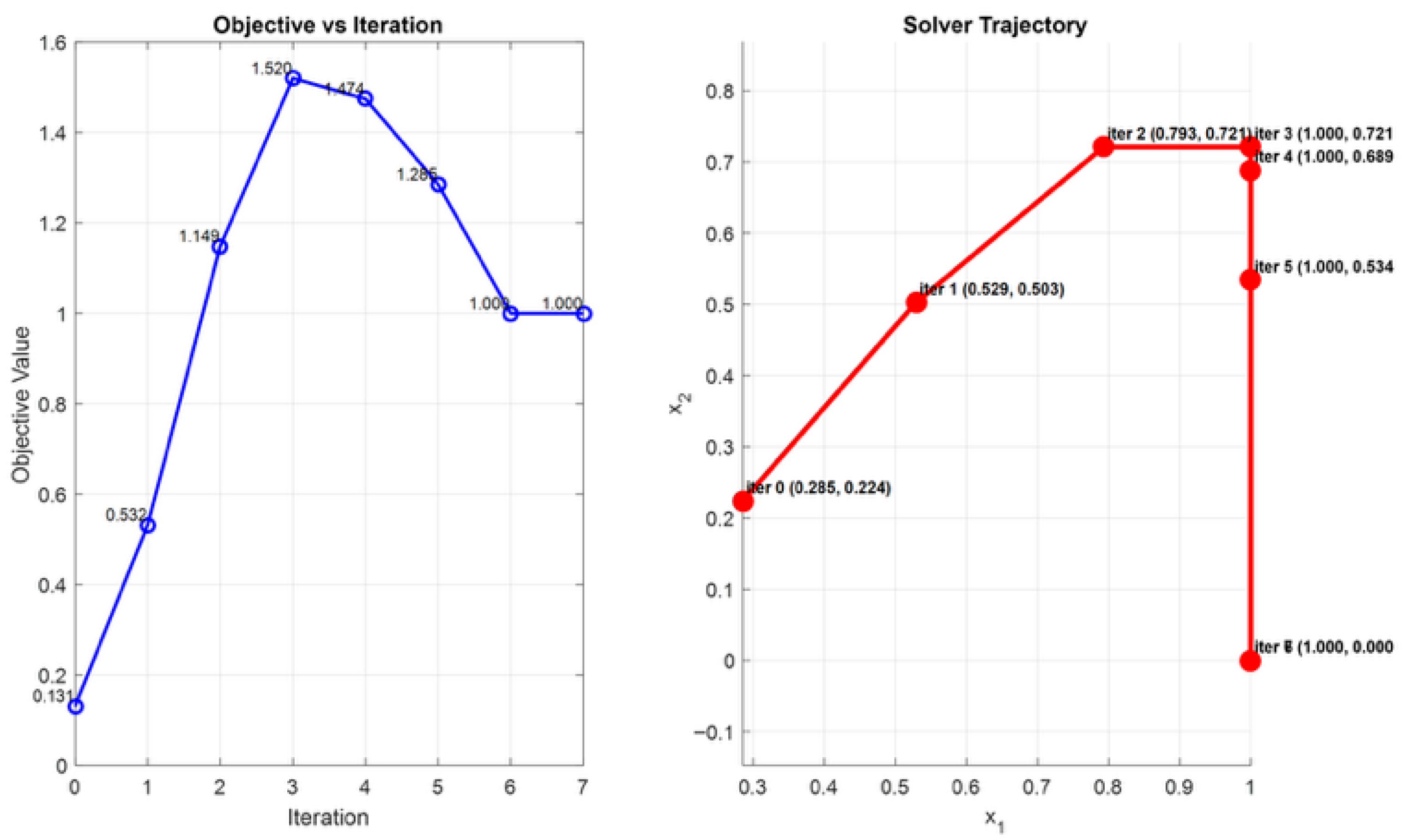
Figure A17.
Objective Function Evaluation and Optimization Progress.
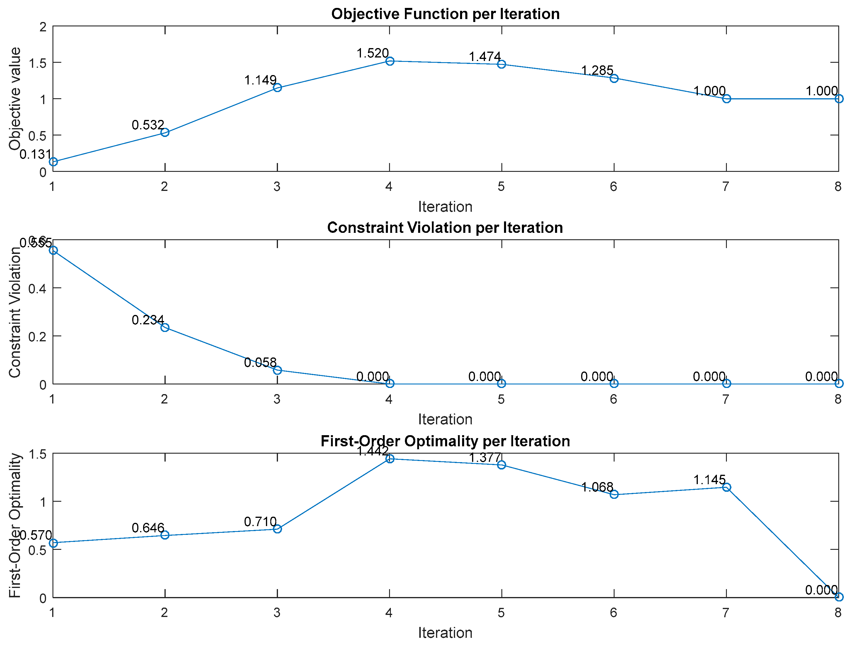
Figure A18.
IPMs iterative trajectory toward feasibility and optimality.
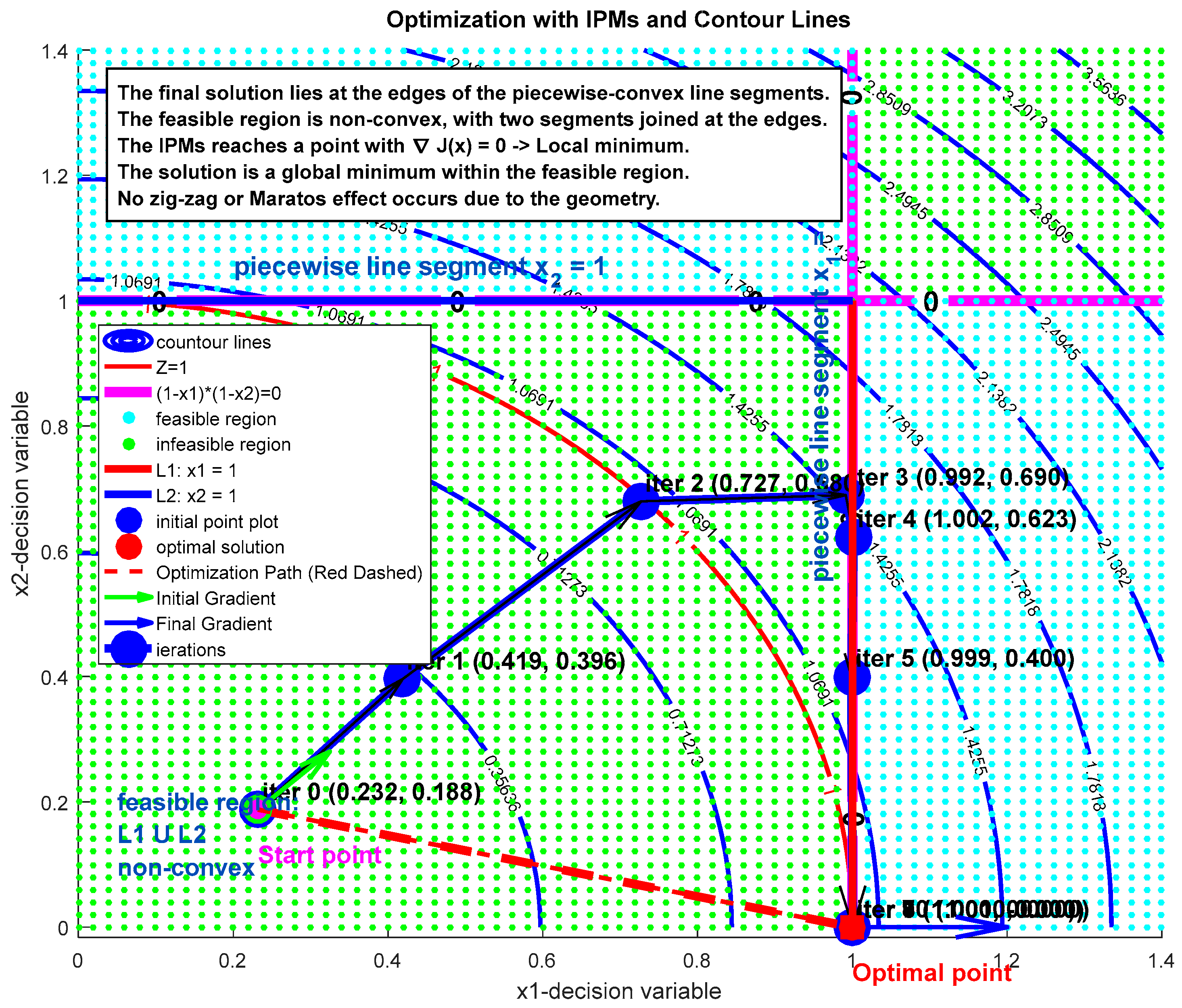
Figure A19.
SQP iterative trajectory toward feasibility and optimality.
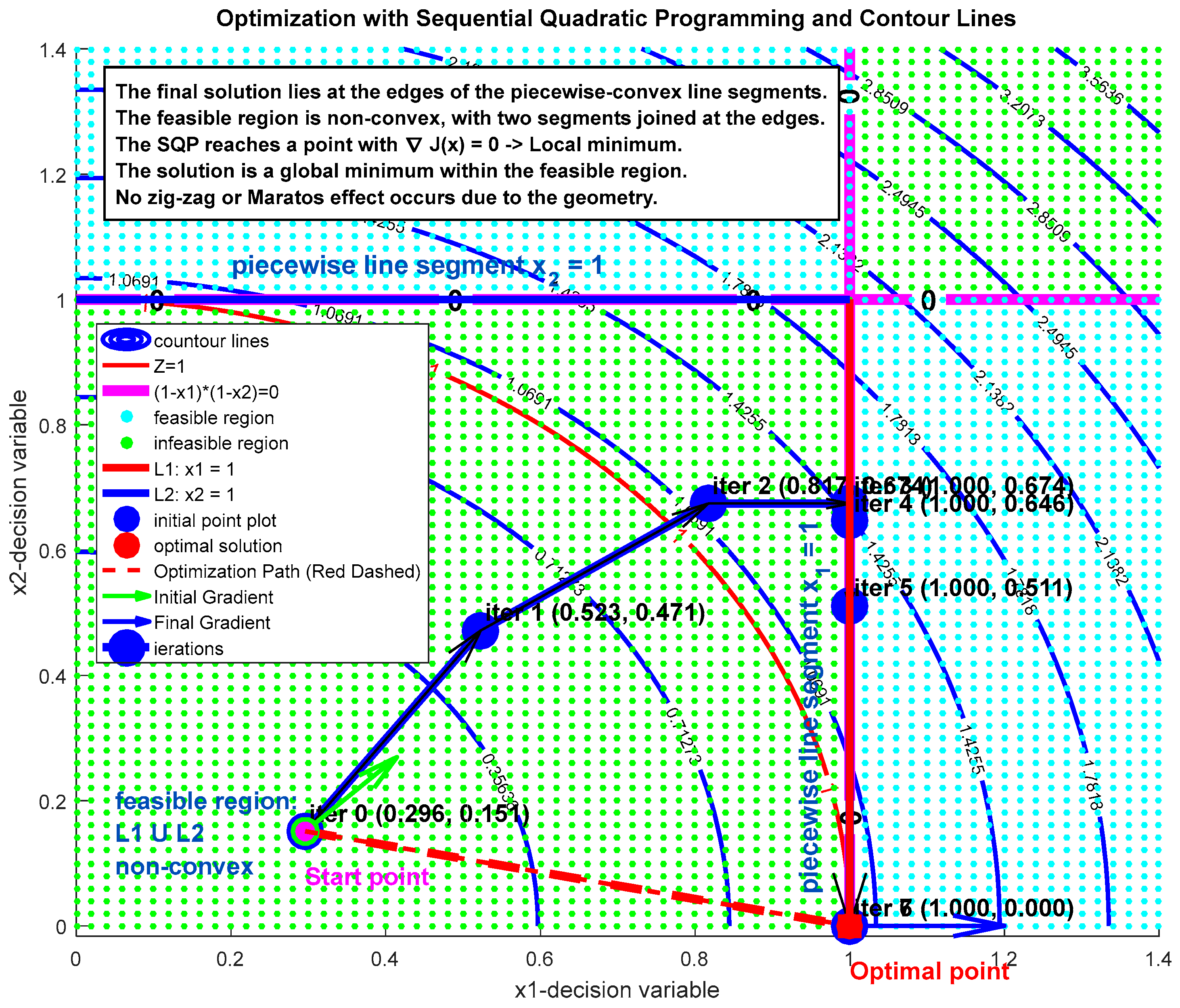
Figure A20.
IPMs iterative trajectory toward feasibility and optimality.
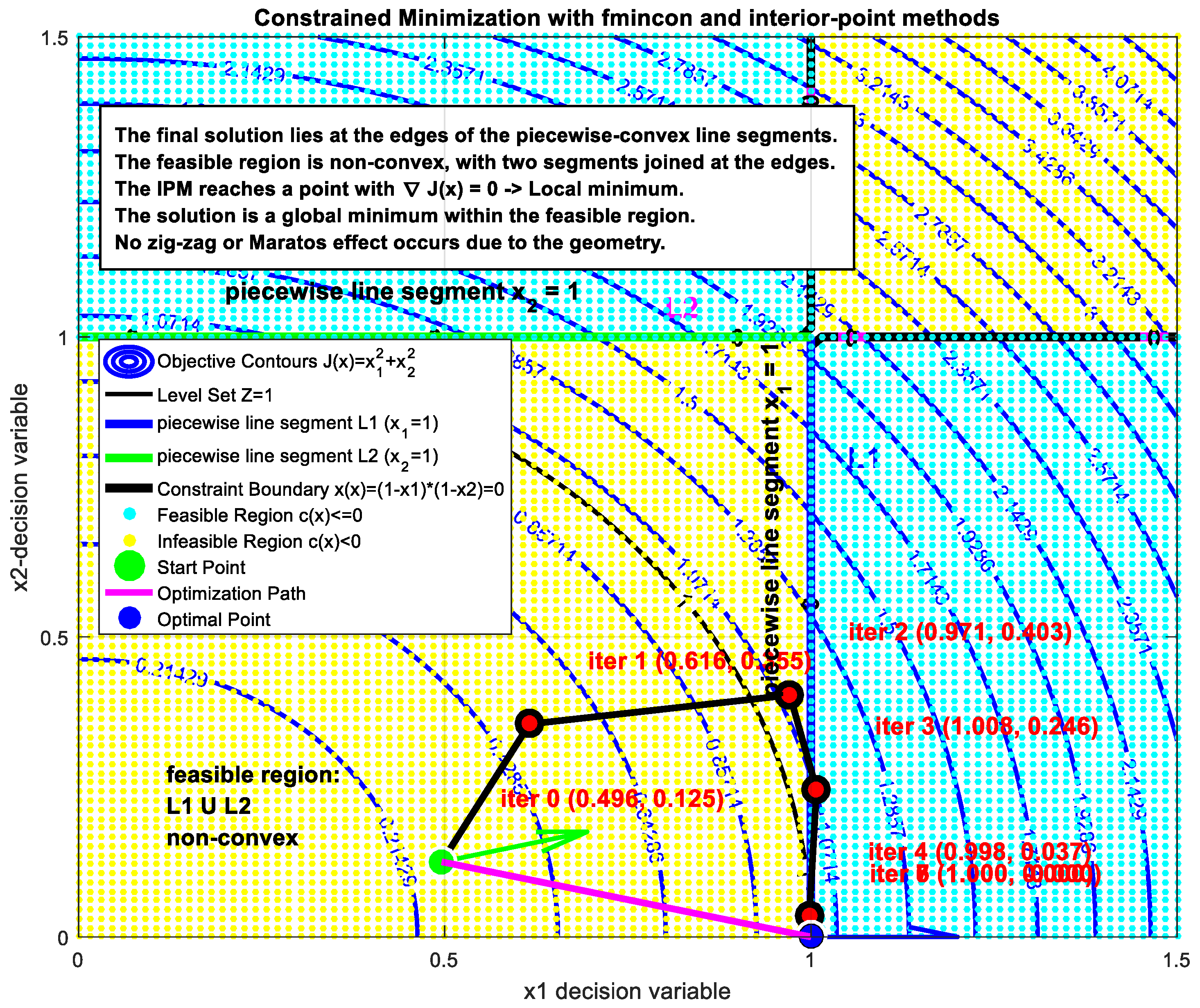
Figure A21.
SQP iterative trajectory toward feasibility and optimality.
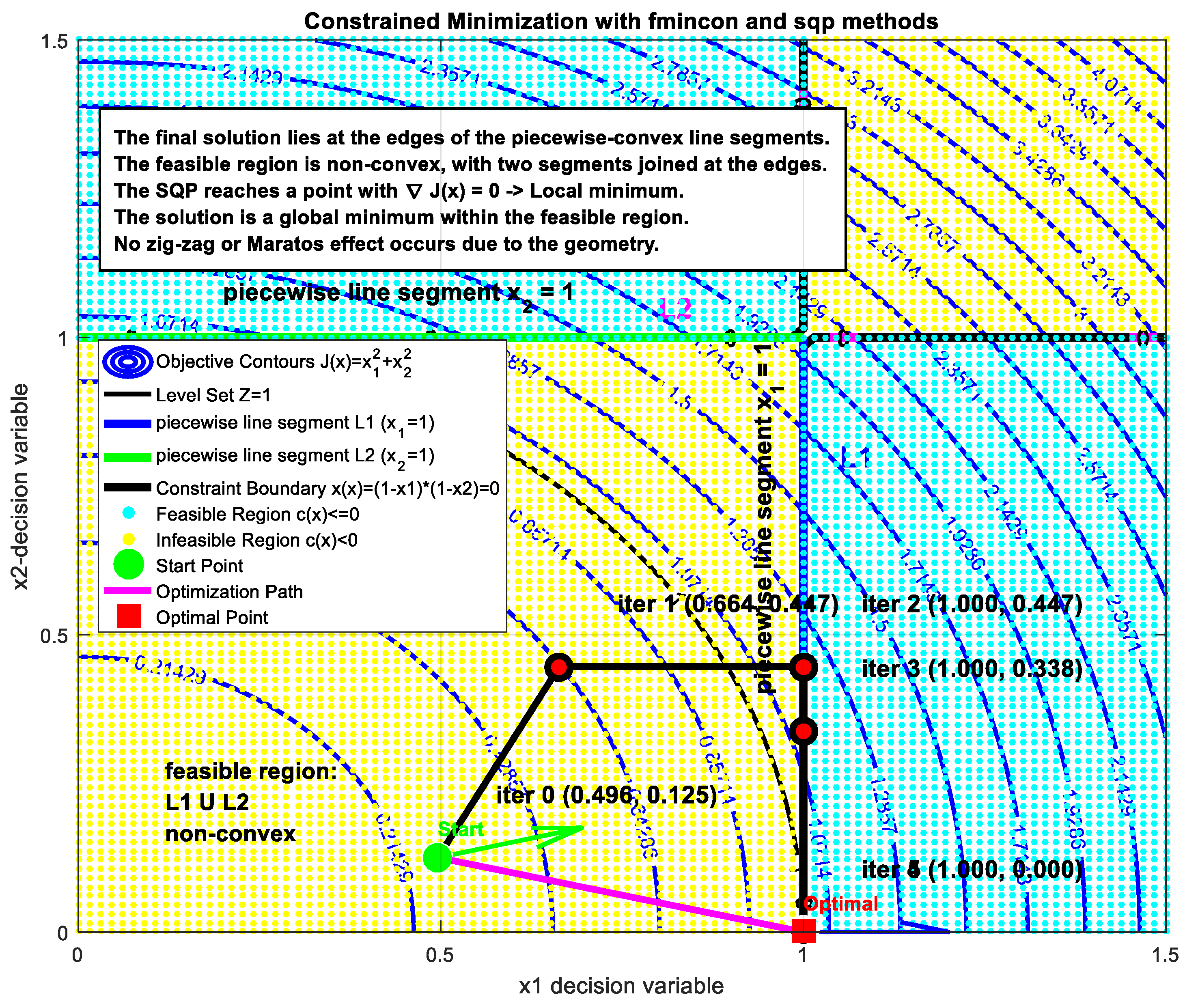
Figure A22.
Ipopt iterative trajectory toward feasibility and optimality.
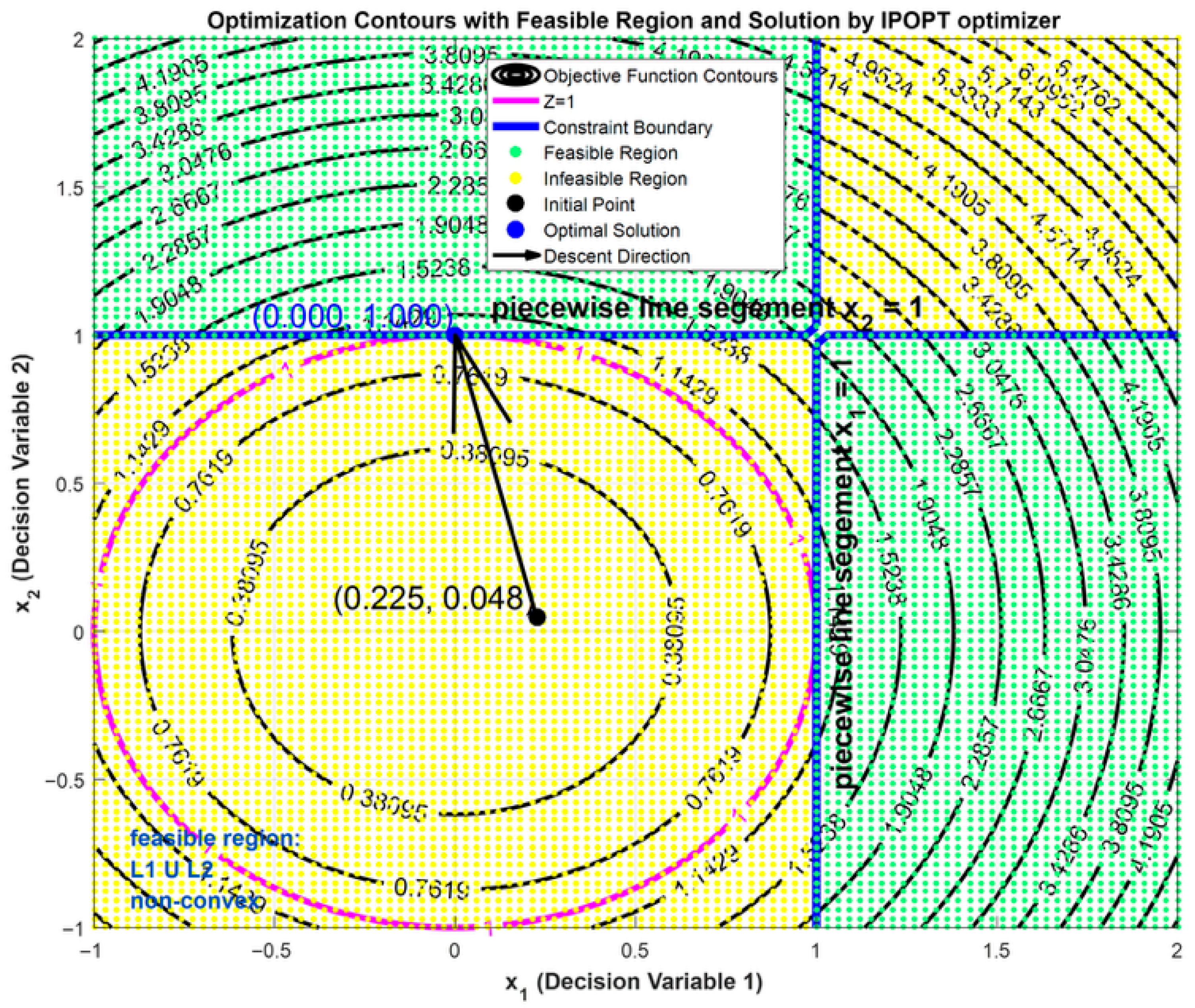
Figure A23.
Ipopt iterative trajectory toward feasibility and optimality.
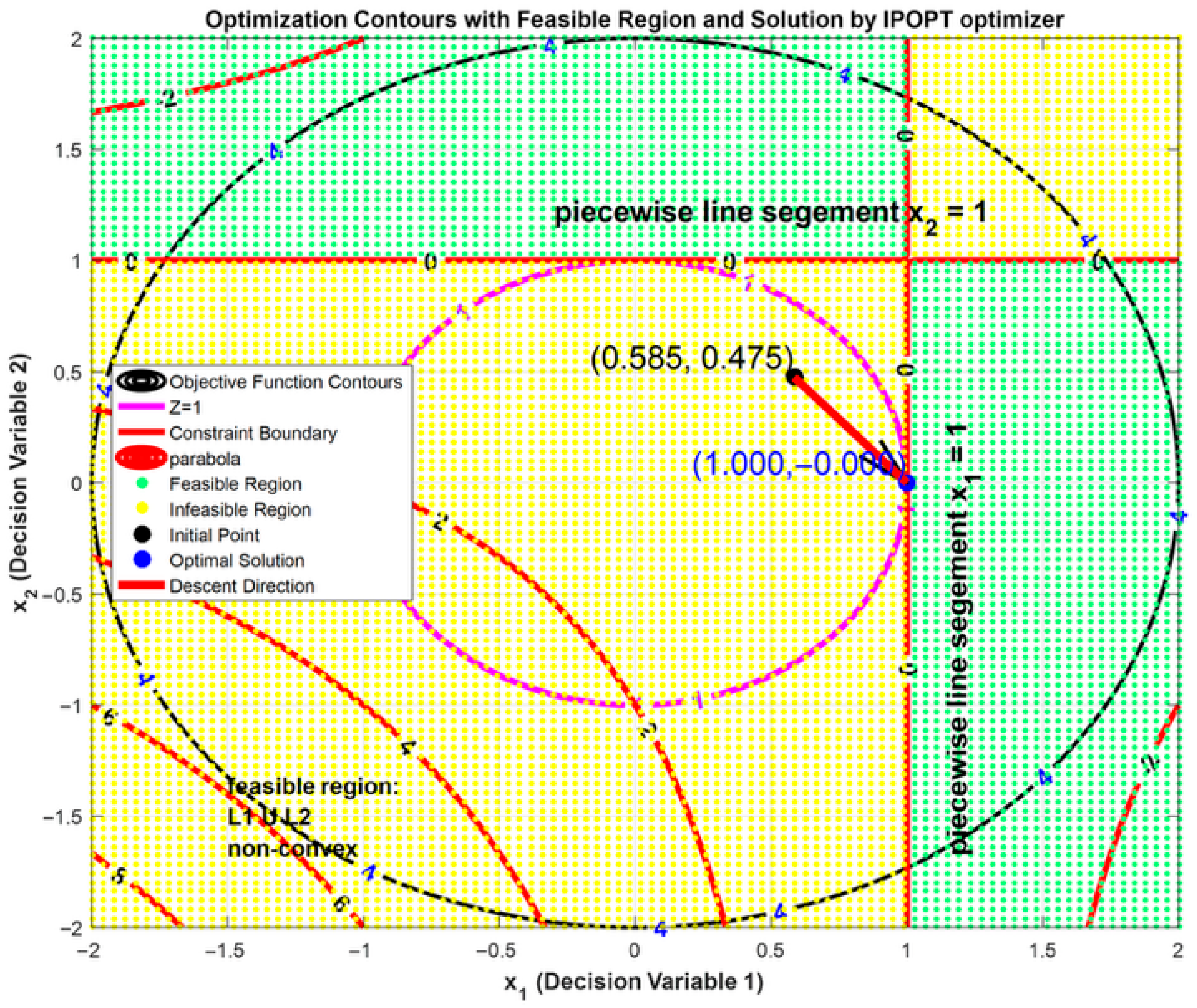
Figure A24.
Ipopt iterative trajectory toward feasibility and optimality.
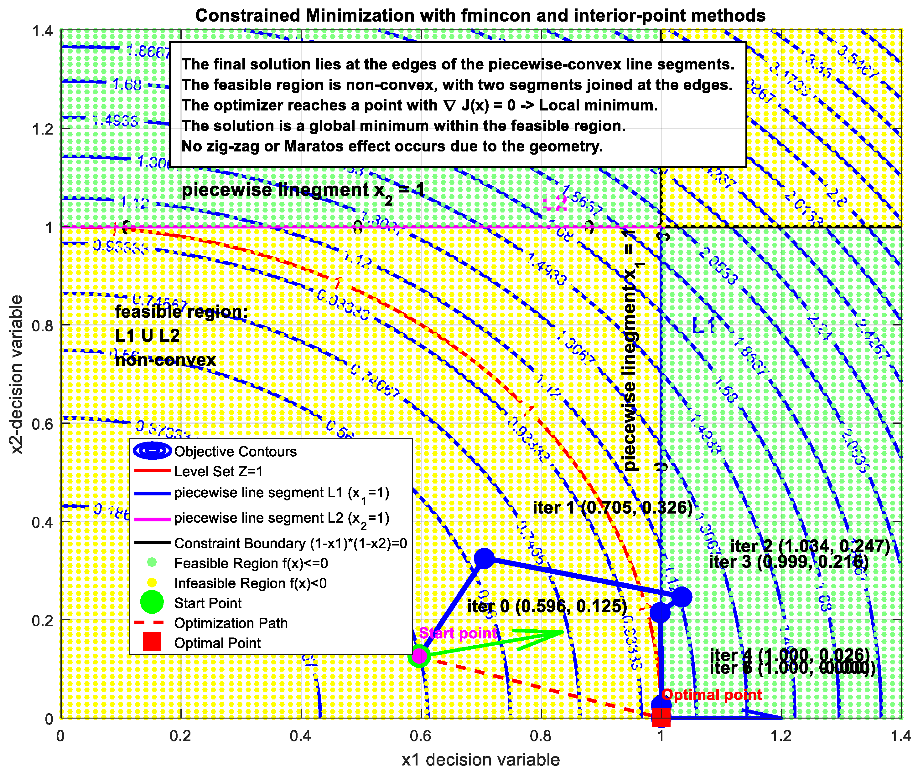
By moving along the line segments, from a certain iteration onward, SQP is able to converge smoothly and monotonically toward the optimal solution (Figure A15, Figure A16 and Figure A17).
SQP takes full steps; feasibility is zero, and the norm of the step decreases without oscillations or reductions in step size. As observed, there are no unnecessary step reductions or regressions near the solution, also proven in our previous works [39,40,58,59].
The line segments in or convex subsets in are crucial to the entire optimization process because local convexity helps preserve feasibility and optimality, thereby helping avoid the Maratos effect, as also evidenced by empirical results in [39,40,55,58,59,96].
The entire feasible region can be viewed as a collection of piecewise-convex subregions, that is, convex subsets in . Starting from an arbitrary initial point, the SQP method in Fmincon reliably converges to the optimal solution located at . As illustrated in Figure A25, this optimal point lies at one of the vertices of the hypercube embedded in .
In convex programming, any local minimum is a global minimum. It makes any locally gradient-based algorithm behave as a global optimizer when solving a convex minimization problem [1,2,3,4,5,6,7,8,74,75,76,77,78,79,80,81,82,83,84,85,86,87,88]. In the specific two-dimensional minimization problem presented here in this study, the feasible region is given by the union of two line segments as displayed in Figure 8, Figure 9, Figure 10, Figure 11, Figure 12, Figure 13, Figure 14, Figure 15, Figure 16 and Figure 17 and Figure A1, Figure A2, Figure A3, Figure A4, Figure A5, Figure A6, Figure A7, Figure A8, Figure A9, Figure A10, Figure A11, Figure A12, Figure A13, Figure A14, Figure A15, Figure A16, Figure A17, Figure A18, Figure A19, Figure A20, Figure A21, Figure A22, Figure A23, Figure A24 and Figure A25.
Although the overall minimization problem is not globally convex, each line segment is convex, with the objective convex function defined in . SQP and IPMs partially explore the search space. Once SQP methods or IPMs capture a line segment, the iterative algorithm effectively solves a convex subproblem along that segment and progresses toward its endpoints, as shown in Figure 8, Figure 9, Figure 10, Figure 11, Figure 12, Figure 13, Figure 14, Figure 15, Figure 16, Figure 17, Figure A1, Figure A2, Figure A3, Figure A4, Figure A5, Figure A6, Figure A7, Figure A8, Figure A9, Figure A10, Figure A11, Figure A12, Figure A13, Figure A14, Figure A15, Figure A16, Figure A17, Figure A18, Figure A19, Figure A20, Figure A21, Figure A22, Figure A23, Figure A24 and Figure A25 [39,40,55,58,59,96].
Figure A25.
SQP Iterative trajectory in Piecewise-Convex Feasible Region in .
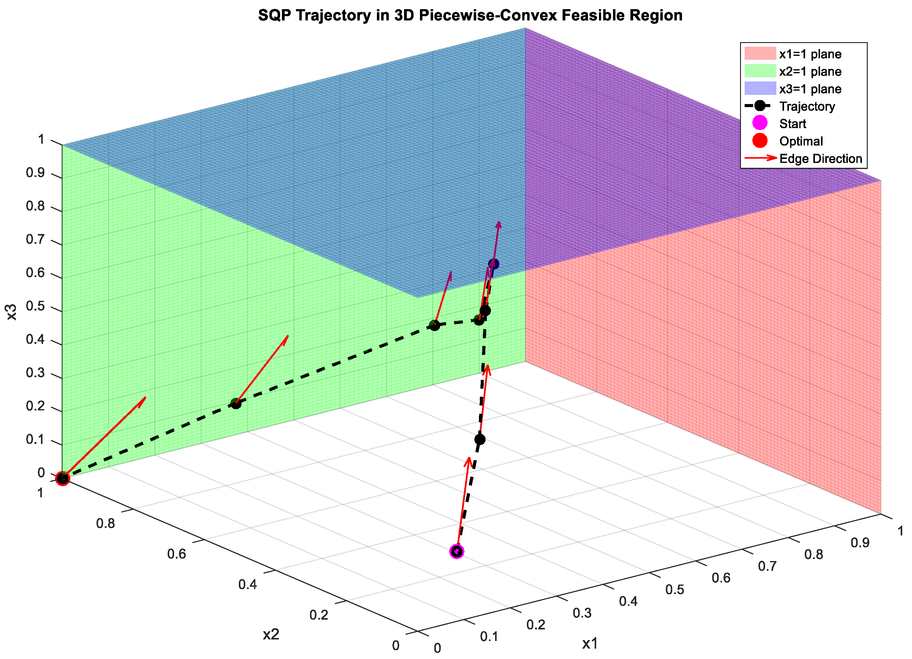
Therefore, the piecewise convexity helps the algorithms to solve the problem globally. As observed, the trajectory plots clearly demonstrate how the iterative algorithms progress monotonically toward the final points or .
SQP and IPMs return a local solution with a step norm equal to zero, and the first-order optimality measure also reaches zero, as shown in the optimization logs [96].
The iterative algorithms yield a local solution that simultaneously satisfies feasibility and optimality. Consequently, the locally gradient-based algorithms locate non-strict local minima that are also non-strict global minima, as also shown in [39,55,58,59,96].
The Maratos effect, which can destroy the superlinear convergence speed due to step rejection near the solution, is effectively avoided, allowing local solutions to be achieved without needing penalty functions. A limitation of the present study is that while the geometric insights are generalized for , the numerical results focus primarily on 2D and 3D benchmark instances. Consequently, the scalability of the piecewise convex decomposition to large-scale power systems (e.g., IEEE 118-bus or 300-bus systems) has not been investigated in this study, although related work is available in [55,58,96].
Nevertheless, similar SQP and IPM performances in MATLAB on larger systems have been explored in our previous work [33,39,40,55,58,59,96], providing evidence that the piecewise convexity approach can effectively produce non-strict global minima while avoiding the Maratos effect, also proven in optimization logs [33,39,55,58,59,96].
The SQP and IPM results are in complete agreement with those obtained using branch-and-bound algorithms, as shown in [33]. Both continuous methods and discrete methods rely on piecewise convexity, relaxations, and relaxed decision bounds [64,98].These approaches produce optimal results, which are also global minima.
Both continuous and discrete approaches yield global solutions, as evidenced by our prior research [33,39,40,55,58,59,96]. Furthermore, recent developments in resilient consensus for discrete-time complex cyber-physical networks under deception attacks are presented in [97]. They provide methods to guarantee convergence even when certain nodes are compromised [98].
This concept is directly relevant to PMU placement, as ensuring full system observability under sensor faults or malicious data requires resilience-aware monitoring. Integrating piecewise convex optimization with resilience considerations can improve both the optimality and robustness of PMU placement in large-scale power systems [96]. This enables accurate and secure state estimation even in the presence of adverse conditions.
In this context, the piecewise convex decomposition of the feasible region enables standard optimization algorithms, such as SQP and IPMs using convexification [100], to converge smoothly to non-strict global minima. These algorithms maintain feasibility throughout the optimization process. They also avoid the Maratos effect, as demonstrated in [33,39,40,55,58,59,96]. By combining these optimization capabilities with resilience-aware design principles, PMU placement strategies can achieve both optimality and robustness, ensuring reliable system observability even under faults or attacks [99].
Appendix D. Justification of Using KKT Optimality Conditions and Multiple Plots
The piecewise convexity of the feasible region in the constrained OPP nonlinear optimization model is not immediately evident from the solutions returned by black-box solvers. A closer examination of the optimization logs is therefore required, as discussed in this paper. We present how the SQP algorithm and interior-point methods avoid the Maratos effect while preserving feasibility [100]. Also, we analyze the constrained nonlinear problem in . By examining the structure of the feasible region in , we observe that the original feasible set can be viewed as a union of line segments or convex subsets [59].
Although this union is non-convex, each individual segment is convex. This decomposition into convex subregions explains why the optimizers behave as in a convex problem, avoiding the Maratos effect along each convex segment, which was also proven in [39,58,59]. Consequently, SQP and IPM generate feasible iterates without requiring any penalty function [75]. To further illustrate the robustness of the SQP and IPM algorithms, Figure 1, Figure 2, Figure 3, Figure 4, Figure 5, Figure 6, Figure 7, Figure 8, Figure 9, Figure 10, Figure 11, Figure 12, Figure 13, Figure 14, Figure 15, Figure 16 and Figure 17 and Figure A1, Figure A2, Figure A3, Figure A4, Figure A5, Figure A6, Figure A7, Figure A8, Figure A9, Figure A10, Figure A11, Figure A12, Figure A13, Figure A14, Figure A15, Figure A16, Figure A17, Figure A18, Figure A19, Figure A20, Figure A21, Figure A22, Figure A23, Figure A24 and Figure A25 present multiple iterative trajectories starting from different initial points.
These plots confirm that independent of the starting position, the algorithms converge smoothly to the endpoints of the convex subregions. This demonstrates the invariance of the convergence path to the initial conditions and highlights the effectiveness of the piecewise convexity approach in guiding the trajectory toward feasible and optimal solutions. As shown in Figure 1, Figure 2, Figure 3, Figure 4, Figure 5, Figure 6, Figure 7, Figure 8, Figure 9, Figure 10, Figure 11, Figure 12, Figure 13, Figure 14, Figure 15, Figure 16 and Figure 17 and Figure A1, Figure A2, Figure A3, Figure A4, Figure A5, Figure A6, Figure A7, Figure A8, Figure A9, Figure A10, Figure A11, Figure A12, Figure A13, Figure A14, Figure A15, Figure A16, Figure A17, Figure A18, Figure A19, Figure A20, Figure A21, Figure A22, Figure A23, Figure A24 and Figure A25, the feasible region consists of two line segments, each of which is convex, although their union is not itself [39,58,59].
No penalty function is required, since feasibility reaches zero after a certain iteration and the optimizer then progresses along one of the segments, thereby avoiding the Maratos effect [39,40,58,59,96]. The objective function decreases monotonically while feasibility remains zero, indicating that no constraint violations occur. Both fmincon and IPOPT exhibit smooth, monotonic convergence toward optimality [39,40,55,58,59,96].
This behavior confirms the absence of oscillations. Full steps are taken during the line search, and superlinear convergence is preserved near the solution. The objective function value decreases consistently toward its optimal value. The optimal solutions are located at the endpoints of the two line segments and are also global optima [33,39,40,58,59,96].
Our analysis demonstrates both analytically and computationally that the SQP and IPM schemes maintain feasibility and optimality simultaneously without the need for penalty terms. Ultimately, the Maratos effect is avoided, and the objective function converges monotonically to the optimal value . The solution lies at the endpoints of the union: or, in higher dimensions, at the vertices of the hypercube in Rⁿ, as shown in Plot 43 for n = 3.
References
- Luenberger, D.G.; Yonge, Y. Linear and Nonlinear Programming, 3rd ed.; Springer: Berlin/Heidelberg, Germany, 2008. [Google Scholar]
- Nocedal, J.; Wright, S. Numerical Optimization; Springer Series in Operations Research and Financial Engineering; Springer: Berlin/Heidelberg, Germany, 2006. [Google Scholar]
- Chinneck, J.W. Feasibility and Infeasibility in Optimization: Algorithms and Computational Methods; International Series in Operations Research and Management Science; Springer: Cham, Switzerland, 2008. [Google Scholar]
- Andrei, N. Continuous Nonlinear Optimization for Engineering Applications in GAMS Technology; Springer Optimization and Its Applications; Springer: Cham, Switzerland, 2017; Volume 121. [Google Scholar]
- Fletcher, R. The Sequential Quadratic Programming Method. In Nonlinear Optimization; Di Pillo, G., Schoen, F., Eds.; Lecture Notes in Mathematics; Springer: Berlin/Heidelberg, Germany, 2010; Volume 1989. [Google Scholar]
- Andrei, N. Interior Point Filter Line Search: IPOPT. In Continuous Nonlinear Optimization for Engineering Applications in GAMS Technology; Springer Optimization and Its Applications; Springer: Cham, Switzerland, 2017; Volume 121, pp. 415–435. [Google Scholar]
- Pirnay, H.; López-Negrete, R.; Biegler, L.T. Optimal Sensitivity Based on IPOPT. Math. Program. Comput. 2012, 4, 307–331. [Google Scholar] [CrossRef] [Scilit]
- Lavezzi, G.; Guye, K.; Cichella, V.; Ciarcià, M. Comparative Analyses of Nonlinear Programming Solvers: Performance Evaluation, Benchmarking, and Multi-UAV Optimal Path Planning. Drones 2023, 7, 487. [Google Scholar] [CrossRef] [Scilit]
- Maratos, N.G.; Moraitis, M.A. Some results on the Sign recurrent neural network for unconstrained minimization. Neurocomputing 2018, 287, 1–21. [Google Scholar] [CrossRef] [Scilit]
- Krasopoulos, P.T.; Maratos, N.G. A Neural Network for Convex Optimization. In Proceedings of the 2006 IEEE International Symposium on Circuits and Systems (ISCAS), Kos, Greece, 21–24 May 2006; p. 4. [Google Scholar]
- Krasopoulos, P.T.; Maratos, N.G. An Interior Point Recurrent Neural Network for Convex Optimization Problems. In Mathematics Without Boundaries; Pardalos, P., Rassias, T., Eds.; Springer: New York, NY, USA, 2014; pp. 1–19. [Google Scholar]
- Barbarosou, M.P.; Maratos, N.G. A Nonfeasible Gradient Projection Recurrent Neural Network for Equality-Constrained Optimization Problems. IEEE Trans. Neural Netw. 2008, 19, 1665–1677. [Google Scholar] [CrossRef] [Scilit]
- Xia, Y.; Feng, G.; Wang, J. A Recurrent Neural Network with Exponential Convergence for Solving Convex Quadratic Programs and Related Linear Piecewise Equations. Neural Netw. 2004, 17, 1003–1015. [Google Scholar] [CrossRef] [Scilit]
- Li, F.; Qin, J.; Kang, Y. Multi-Agent System Based Distributed Pattern Search Algorithm for Non-Convex Economic Load Dispatch in Smart Grid. IEEE Trans. Power Syst. 2019, 34, 2093–2102. [Google Scholar] [CrossRef] [Scilit]
- Yang, T.; Binh, N.T.; Thang, T.M.; Hoa, D.T. A New Smoothing Nonlinear Penalty Function for Constrained Optimization. Math. Comput. Appl. 2017, 22, 31. [Google Scholar] [CrossRef] [Scilit]
- Liu, W.; Yang, L.; Yu, B. A Lifting-Penalty Method for Quadratic Programming with a Quadratic Matrix Inequality Constraint. Mathematics 2020, 8, 153. [Google Scholar] [CrossRef] [Scilit]
- Fletcher, R. Penalty Functions. In Mathematical Programming: The State of the Art; Bachem, A., Korte, B., Grötschel, M., Eds.; Springer: Berlin/Heidelberg, Germany, 1983; pp. 87–114. [Google Scholar]
- Wang, L.; Sun, Y.; Sun, J.; Yuan, Y.; Wang, B. Optimality Conditions and Stability Analyses for the Second-Order Cone Constrained Variational Inequalities. Axioms 2025, 14, 342. [Google Scholar] [CrossRef] [Scilit]
- Ruiz-Garzón, G.; Ruiz-Zapatero, J.; Osuna-Gómez, R.; Rufián-Lizana, A. Necessary and Sufficient Second-Order Optimality Conditions on Hadamard Manifolds. Mathematics 2020, 8, 1152. [Google Scholar] [CrossRef] [Scilit]
- Liao, J.; Wan, Z. Inexact Restoration Methods for Semivectorial Bilevel Programming Problem on Riemannian Manifolds. Axioms 2022, 11, 696. [Google Scholar] [CrossRef] [Scilit]
- Kaliyaperumal, P.; Das, A. A Mathematical Model for Nonlinear Optimization Which Attempts Membership Functions to Address the Uncertainties. Mathematics 2022, 10, 1743. [Google Scholar] [CrossRef] [Scilit]
- Wang, S.; Wang, X.; Tian, Y.; Pang, L. A New Hybrid Descent Algorithm for Large-Scale Nonconvex Optimization and Application to Some Image Restoration Problems. Mathematics 2024, 12, 3088. [Google Scholar] [CrossRef] [Scilit]
- Lai, K.K.; Mishra, S.K.; Sharma, R.; Sharma, M.; Ram, B. A Modified q-BFGS Algorithm for Unconstrained Optimization. Mathematics 2023, 11, 1420. [Google Scholar] [CrossRef] [Scilit]
- Levin, D.; Gruberger, N. Adapted B-Spline Quasi-Interpolation for Approximating Piecewise Smooth Functions. Algorithms 2025, 18, 335. [Google Scholar] [CrossRef] [Scilit]
- Syzonov, O.; Tomasiello, S.; Capuano, N. New Insights into Fuzzy Genetic Algorithms for Optimization Problems. Algorithms 2024, 17, 549. [Google Scholar] [CrossRef] [Scilit]
- Liu, C.-S.; Kuo, C.-L.; Chang, C.-W. Solving Least-Squares Problems via a Double-Optimal Algorithm and a Variant of the Karush–Kuhn–Tucker Equation for Over-Determined Systems. Algorithms 2024, 17, 211. [Google Scholar] [CrossRef] [Scilit]
- El-Sobky, B.; Abo-Elnaga, Y.; Mousa, A.A.A.; El-Shorbagy, M.A. Trust-Region Based Penalty Barrier Algorithm for Constrained Nonlinear Programming Problems: An Application of Design of Minimum Cost Canal Sections. Mathematics 2021, 9, 1551. [Google Scholar] [CrossRef] [Scilit]
- Chen, M.; Zhou, Y.; Luo, Q. An Improven Arithmetic Optimization Algorithm for Numerical Optimization Problems. Mathematics 2022, 10, 2152. [Google Scholar] [CrossRef] [Scilit]
- Johnson, T.; Moger, T. A critical review of methods for optimal placement of phasor measurement units. Int. Trans. Electr. Energy Syst. 2020, 31, e12698. [Google Scholar] [CrossRef] [Scilit]
- Ahmed, M.M.; Amjad, M.; Qureshi, M.A.; Imran, K.; Haider, Z.M.; Khan, M.O. A Critical Review of State-of-the-Art Optimal PMU Placement Techniques. Energies 2022, 15, 2125. [Google Scholar] [CrossRef] [Scilit]
- Biswal, C.; Sahu, B.K.; Mishra, M.; Rout, P.K. Real-Time Grid Monitoring and Protection: A Comprehensive Survey on the Advantages of Phasor Measurement Units. Energies 2023, 16, 4054. [Google Scholar] [CrossRef] [Scilit]
- Paramo, G.; Bretas, A.; Meyn, S. Research Trends and Applications of PMUs. Energies 2022, 15, 5329. [Google Scholar] [CrossRef] [Scilit]
- Theodorakatos, N.P.; Babu, R.; Moschoudis, A.P. The branch-and-bound algorithm in optimizing mathematical programming models to achieve power grid observability. Axioms 2023, 12, 1040. [Google Scholar] [CrossRef] [Scilit]
- Dua, D.; Dambhare, S.; Gajbhiye, R.K.; Soman, S.A. Optimal Multistage Scheduling of PMU Placement: An ILP Approach. IEEE Trans. Power Deliv. 2008, 23, 1812–1820. [Google Scholar] [CrossRef] [Scilit]
- Elsayed, A.A.E.; Farag, H.E.Z. A Novel Optimal Placement of Multi-Type Sensors for Smart Grids Observability Using an Enhanced Graph Theory Search Algorithm. In Proceedings of the 2025 IEEE 34th International Symposium on Industrial Electronics (ISIE), Toronto, ON, Canada, 20–23 June 2025; pp. 1–6. [Google Scholar]
- Elsayed, A.A.E.; Khalaf, M.; Mohamed, M.A.; Nayel, M.A.E.; Kundur, D. Optimal Multi-Type Sensor Placement Using Hybrid Graph Theory and Numerical Observability Analyses for System Observability and Cybersecurity Enhancement. Electr. Power Syst. Res. 2025, 241, 111361. [Google Scholar] [CrossRef] [Scilit]
- Ahmed, M.M.; Amjad, M.; Qureshi, M.A.; Khan, M.O.; Haider, Z.M. Optimal PMU Placement to Enhance Observability in Transmission Networks Using ILP and Degree of Centrality. Energies 2024, 17, 2140. [Google Scholar] [CrossRef] [Scilit]
- Hu, S.; Hu, G.; Du, B.; Hussien, A.G. A Novel Artificial Eagle-Inspired Optimization Algorithm for Trade Hub Location and Allocation Method. Biomimetics 2025, 10, 481. [Google Scholar] [CrossRef] [Scilit]
- Theodorakatos, N.P.; Babu, R.; Theodoridis, C.A.; Moschoudis, A.P. Mathematical Models for the Single-Channel and Multi-Channel PMU Allocation Problem and Their Solution Algorithms. Algorithms 2024, 17, 191. [Google Scholar] [CrossRef] [Scilit]
- Theodorakatos, N.P.; Lytras, M.; Babu, R. A Generalized Pattern Search Algorithm Methodology for Solving an Under-Determined System of Equality Constraints to Achieve Power System Observability Using Synchrophasors. J. Phys. Conf. Ser. 2021, 2090, 012125. [Google Scholar] [CrossRef] [Scilit]
- Hamid Hosseini Dolatabadi, S.; Bhuiyan, T.H.; Golshan, M.E.H. A Heuristic Solution Algorithm for a Comprehensive Optimal Phasor Measurement Unit Placement Considering Zero-Injection Buses and Practical Constraints in Power System State Observability Problem. IEEE Access 2024, 12, 79919–79936. [Google Scholar] [CrossRef] [Scilit]
- Koutsoukis, N.C.; Manousakis, N.M.; Georgilakis, P.S.; Korres, G.N. Numerical observability method for optimal phasor measurement units placement using recursive Tabu search method. IET Gener. Transm. Distrib. 2013, 7, 347–356. [Google Scholar] [CrossRef] [Scilit]
- Müller, H.H.; Castro, C.A. Genetic algorithm-based phasor measurement unit placement method considering observability and security criteria. IET Gener. Transm. Distrib. 2016, 10, 270–280. [Google Scholar] [CrossRef] [Scilit]
- Singh, S.P.; Singh, S.P. A Multi-objective PMU Placement Method in Power System via Binary Gravitational Search Algorithm. Electr. Power Compon. Syst. 2017, 45, 1832–1845. [Google Scholar] [CrossRef] [Scilit]
- Zhang, S.; Hu, X.; Gao, Y.; Gao, M.; Zhang, Y. Exemplar Learning and Memory Retrieval-Based Particle Swarm Optimization Algorithm with Engineering Applications. Biomimetics 2025, 10, 708. [Google Scholar] [CrossRef] [Scilit]
- Carvajal, G.; Carrión, D.; Jaramillo, M. Planning Scheme for Optimal PMU Location Considering Power System Expansion. Energies 2025, 18, 3283. [Google Scholar] [CrossRef] [Scilit]
- Upadhyay, B.B.; Singh, S.K.; Stancu-Minasian, I. Constraint Qualifications and Optimality Conditions for Nonsmooth Semidefinite Multiobjective Programming Problems with Mixed Constraints Using Convexificators. Mathematics 2024, 12, 3202. [Google Scholar] [CrossRef] [Scilit]
- Korres, G.N.; Manousakis, N.M.; Xygkis, T.C.; Lofberg, J. Optimal phasor measurement unit placement for numerical observability in the presence of conventional measurement using semi-definite programming. IET Gener. Transm. Distrib. 2015, 9, 2427–2436. [Google Scholar] [CrossRef] [Scilit]
- Manousakis, N.M.; Korres, G.N. Optimal PMU placement for numerical observability considering fixed channel capacity—A semidefinite programming approach. IEEE Trans. Power Syst. 2016, 31, 3328–3329. [Google Scholar] [CrossRef] [Scilit]
- Manousakis, N.M.; Korres, G.N. Semidefinite programming for optimal placement of PMUs with channel limits considering pre-existing SCADA and PMU measurements. In Proceedings of the 2016 Power Systems Computation Conference (PSCC), Genoa, Italy, 20–24 June 2016. [Google Scholar]
- Manousakis, N.M.; Korres, G.N. Optimal PMU arrangement considering limited channel capacity and transformer tap settings. IET Gener. Transm. Distrib. 2020, 14, 5984–5991. [Google Scholar] [CrossRef] [Scilit]
- Xygkis, T.C.; Löfberg, J.; Korres, G.N. Investigation of Optimal Phasor Measurement Selection for Distribution System State Estimation Under Various Uncertainties. IEEE Trans. Instrum. Meas. 2025, 74, 9006616. [Google Scholar] [CrossRef] [Scilit]
- Almunif, A.; Fan, L. DC State Estimation Model-Based Mixed Integer Semidefinite Programming for Optimal PMU Placement. In Proceedings of the 2018 North American Power Symposium (NAPS), Fargo, ND, USA, 9–11 September 2018; pp. 1–6. [Google Scholar]
- Manousakis, N.M.; Korres, G.N. A Weighted Least Squares Algorithm for optimal PMU placement. IEEE Trans. Power Syst. 2013, 28, 3499–3500. [Google Scholar] [CrossRef] [Scilit]
- Theodorakatos, N.P.; Manousakis, N.M.; Korres, G.N. Optimal Placement of Phasor Measurement Units with Linear and Non-linear Models. Electr. Power Compon. Syst. 2015, 43, 357–373. [Google Scholar] [CrossRef] [Scilit]
- Almunif, A.; Fan, L. Mixed integer linear programming and nonlinear programming for optimal PMU placement. In Proceedings of the 2017 North American Power Symposium (NAPS), Morgantown, WV, USA, 17–19 September 2017; pp. 1–6. [Google Scholar]
- Almunif, A.; Fan, L. Optimal PMU placement for modeling power grid observability with mathematical programming methods. Int. Trans. Electr. Energy Syst. 2020, 30, e12182. [Google Scholar] [CrossRef] [Scilit]
- Theodorakatos, N.P.; Lytras, M.; Babu, R. Toward Smart Energy Grids: A Box-Constrained Nonlinear Underdetermined Model for Power System Observability Using Recursive Quadratic Programming. Energies 2020, 13, 1724. [Google Scholar] [CrossRef] [Scilit]
- Theodorakatos, N.P.; Babu, R. Hybrid Optimization Strategies for Global Optimality in Non-Convex Programming Using SQP and IPMs: Avoiding the Maratos effect in PMU Placement—A Case Study. J. Phys. Conf. Ser. 2025, 3027, 012041. [Google Scholar] [CrossRef] [Scilit]
- Bečejac, V.; Stefanov, P. Groebner bases algorithm for optimal PMU placement. Int. J. Electr. Power Energy Syst. 2020, 115, 105427. [Google Scholar] [CrossRef] [Scilit]
- Yildiz, T.; Abur, A. Sparse PMU placement algorithm for enhanced detection and identification of power grid events. IEEE Trans. Power Syst. 2025, 40, 1843–1853. [Google Scholar] [CrossRef] [Scilit]
- Miller, T.; Durlik, I.; Kostecka, E.; Kozlovska, P.; Nowak, A. Federated Learning for Decentralized Electricity Market Optimization: A Review and Research Agenda. Energies 2025, 18, 4682. [Google Scholar] [CrossRef] [Scilit]
- Ali, Z.M.; Razavi, S.E.; Javadi, M.S.; Gandoman, F.H.; Abdel Aleem, S.H. Dual enhancement of power system monitoring: Improven probabilistic multi-stage PMU placement with an increased search space and mathematical linear expansion to consider zero-injection bus. Energies 2018, 11, 1429. [Google Scholar] [CrossRef] [Scilit]
- Moutis, P.; Thakar, P. Stochasticity agnostic solution to the AC optimal power flow by recursive bound tightening with top-down heuristically inducted binary decision trees. IET Gener. Transm. Distrib. 2023, 17, 102–115. [Google Scholar] [CrossRef] [Scilit]
- Mandal, A.K.; De, S.; Panigrahi, B.K. Grid Controllability Aware Optimal Placement of PMUs with Limited Input Current Channels. IEEE Trans. Ind. Appl. 2024, 60, 8532–8547. [Google Scholar] [CrossRef] [Scilit]
- Lythgoe, Z.J.; Long, T.F.; Buchholz, M.J.; Livernois, A.R.; Kanuteh, K.; Allee, D.R.; Pal, A.; Graham, I.R.; Drummond, Z.D. Design and Validation of a Very Low-Power Phasor Measurement Unit for the Distribution System. IEEE Trans. Ind. Appl. 2025, 61, 3553. [Google Scholar] [CrossRef] [Scilit]
- Varghese, A.C.; Shah, H.; Azimian, B.; Pal, A.; Farantatos, E. Deep Neural Network-Based State Estimator for Transmission System Considering Practical Implementation Challenges. J. Mod. Power Syst. Clean Energy 2024, 12, 1810–1822. [Google Scholar] [CrossRef] [Scilit]
- Sarjan, H.; Asghari, M.; Ameli, A.; Ghafouri, M. Mitigating Propagation of Cyber-Attacks in Wide-Area Measurement Systems. IEEE Trans. Inf. Forensics Secur. 2024, 19, 9984–9999. [Google Scholar] [CrossRef] [Scilit]
- Bae, J. Cost-Effective placement of phasor measurement units to defend against false data injection attacks on power grid. Energies 2020, 13, 3862. [Google Scholar] [CrossRef] [Scilit]
- Luo, C.; Zhou, Z.; Jiang, R.; Zheng, B. Attentional Convolutional Neural Network Based on Distinction Enhancement and Information Fusion for FDIA Detection in Power Systems. Electronics 2024, 13, 4862. [Google Scholar] [CrossRef] [Scilit]
- Al-Sharawi, R.; Ali, A.; Shaaban, M.; Qaddoumi, N.; Abdalzaher, M.S. Tackling the Optimal Phasor Measurement Unit Placement and Attack Detection Problems in Smart Grids by Incorporating Machine Learning. IEEE Open J. Commun. Soc. 2025, 6, 4036–4050. [Google Scholar] [CrossRef] [Scilit]
- Resende, E.; Pires, R.; Mili, L. New Topological Observability Algorithm for Hybrid Power System Static State Estimation. J. Mod. Power Syst. Clean Energy 2024, 13, 1945–1954. [Google Scholar] [CrossRef] [Scilit]
- Qin, J.; Wan, Y.; Li, F.; Kang, Y.; Fu, W. Distributed Economic Operation in Smart Grid: Model-Based and Model-Free Perspectives; Studies in Systems, Decision and Control; Springer: Singapore, 2021. [Google Scholar]
- Maratos, N.G. Exact Penalty Function Algorithms for Finite Dimensional and Optimization Problems. Ph.D. Thesis, Imperial College of Science and Technology, University of London, London, UK, 1978. [Google Scholar]
- Mayne, D.Q.; Maratos, N. A First Order, Exact Penalty Function Algorithm for Equality Constrained Optimization Problems. Math. Program. 1979, 16, 303–324. [Google Scholar] [CrossRef] [Scilit]
- Pantoja, J.F.A.D.O.; Mayne, D.Q. Exact penalty function algorithm with simple updating of the penalty parameter. J. Optim. Theory Appl. 1991, 69, 441–467. [Google Scholar] [CrossRef] [Scilit]
- Fabien, B.C. Implementation of a Robust SQP Algorithm. Optim. Methods Softw. 2008, 23, 827–846. [Google Scholar] [CrossRef] [Scilit]
- Andrei, N. A SQP Method Using Only Equality-Constrained Sub-Problems: DONLP. In Continuous Nonlinear Optimization for Engineering Applications in GAMS Technology; Springer Optimization and Its Applications; Springer: Cham, Switzerland, 2017; Volume 121. [Google Scholar]
- Chamberlain, R.M.; Powell, M.J.D.; Lemaréchal, C.; Pedersen, H.C. The Watchdog Technique for Forcing Convergence in Algorithms for Constrained Minimization. Math. Program. Study 1982, 16, 1–17. [Google Scholar]
- Byrd, R.; Schnabel, R.; Shultz, G. A Trust Region Algorithm for Nonlinearly Constrained Optimization. SIAM J. Numer. Anal. 1987, 24, 1152–1170. [Google Scholar] [CrossRef] [Scilit]
- Wächter, A.; Biegler, L.T. Line Search Filter Methods for Nonlinear Programming: Motivation and Global Convergence. SIAM J. Optim. 2005, 16, 1–31. [Google Scholar] [CrossRef] [Scilit]
- Wächter, A.; Biegler, L.T. On the Implementation of an Interior-Point Filter Line-Search Algorithm for Large-Scale Nonlinear Programming. Math. Program. 2006, 106, 25–57. [Google Scholar] [CrossRef] [Scilit]
- Nocedal, J.; Öztoprak, F.; Waltz, R.A. An interior point method for nonlinear programming with infeasibility detection capabilities. Optim. Methods Softw. 2013, 29, 837–854. [Google Scholar] [CrossRef] [Scilit]
- Yamakawa, Y. A Stabilized Sequential Quadratic Programming Method for Optimization Problems in Function Spaces. Numer. Funct. Anal. Optim. 2023, 44, 1–39. [Google Scholar] [CrossRef] [Scilit]
- Jian, J.B.; Tang, C.M.; Hu, Q.J.; Han, D.L. A Sequential Quadratic Programming Algorithm Without a Penalty Function, a Filter or a Constraint Qualification for Inequality Constrained Optimization. Optimization 2020, 69, 1603–1635. [Google Scholar] [CrossRef] [Scilit]
- Ahmadzadeh, H.; Mahdavi-Amiri, N. A Competitive Inexact Nonmonotone Filter SQP Method: Convergence Analyses and Numerical Results. Optim. Methods Softw. 2021, 36, 867–905. [Google Scholar] [CrossRef] [Scilit]
- Panier, E.R.; Tits, A.L. Avoiding the Maratos Effect by Means of a Nonmonotone Line Search I. General Constrained Problems. SIAM J. Numer. Anal. 1991, 28, 1183–1195. [Google Scholar] [CrossRef] [Scilit]
- Fletcher, R.; Leyffer, S. Nonlinear Programming Without a Penalty Function. Math. Program. 2002, 91, 239–269. [Google Scholar] [CrossRef] [Scilit]
- The MathWorks Inc. Optimization Toolbox for Use with MATLAB R®. User’s Guide for Mathwork. 2016. Available online: www.mathworks.com (accessed on 10 October 2025).
- Available online: https://coin-or.github.io/Ipopt/ (accessed on 10 October 2025).
- Available online: https://www.mathworks.com/help/optim/ug/fmincon.html (accessed on 10 October 2025).
- Zimmerman, R.D.; Murillo-Sánchez, C.E.; Thomas, R.J. MATPOWER: Steady-state operations, planning, and analyses tools for power systems research and education. IEEE Trans. Power Syst. 2010, 26, 12–19. [Google Scholar] [CrossRef] [Scilit]
- Available online: https://icseg.iti.illinois.edu/power-cases/ (accessed on 10 October 2025).
- Du, Z.; Yin, H.; Zhang, X.; Hu, H.; Liu, T.; Hou, M.; Giannelos, S.; Strbac, G. Decarbonisation of Data Centre Networks Through Computing Power Migration. In Proceedings of the 2025 IEEE 5th International Conference on Computer Communication and Artificial Intelligence (CCAI), Haikou, China, 23–25 May 2025; pp. 871–876. [Google Scholar]
- Kaloev, M.; Krastev, G. Comprehensive Review of Benefits from the Use of Sparse Updates Techniques in Reinforcement Learning: Experimental Simulations in Complex Action Space Environments. In Proceedings of the 2023 4th International Conference on Communications, Information, Electronic and Energy Systems (CIEES), Plovdiv, Bulgaria, 23–25 November 2023; pp. 1–7. [Google Scholar]
- Theodorakatos, N.P.; Lytras, M.D.; Moschoudis, A.P.; Kantoutsis, K.T. Implementation of optimization-based algorithms for maximum power system observability using synchronized measurements. AIP Conf. Proc. 2023, 2872, 120006. [Google Scholar] [CrossRef] [Scilit]
- Fu, W.; Qin, J.; Shi, Y.; Zheng, W.X.; Kang, Y. Resilient consensus of discrete-time complex cyber-physical networks under deception attacks. IEEE Trans. Ind. Inform. 2020, 16, 4868–4877. [Google Scholar] [CrossRef] [Scilit]
- Available online: https://www.minlp.com/baron-solver (accessed on 4 December 2025).
- Qin, J.; Li, M.; Wang, J.; Shi, L.; Kang, Y.; Zheng, W.X. Optimal denial-of-service attack energy management against state estimation over an SINR-based network. Automatica 2020, 119, 109090. [Google Scholar] [CrossRef] [Scilit]
- Zhang, Y.; Sahinidis, N.V. Solving Continuous and Discrete Nonlinear Programs with BARON. Comput. Optim. Appl. 2025, 92, 1123–1161. [Google Scholar] [CrossRef] [Scilit]
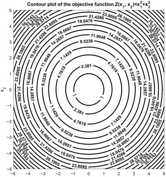
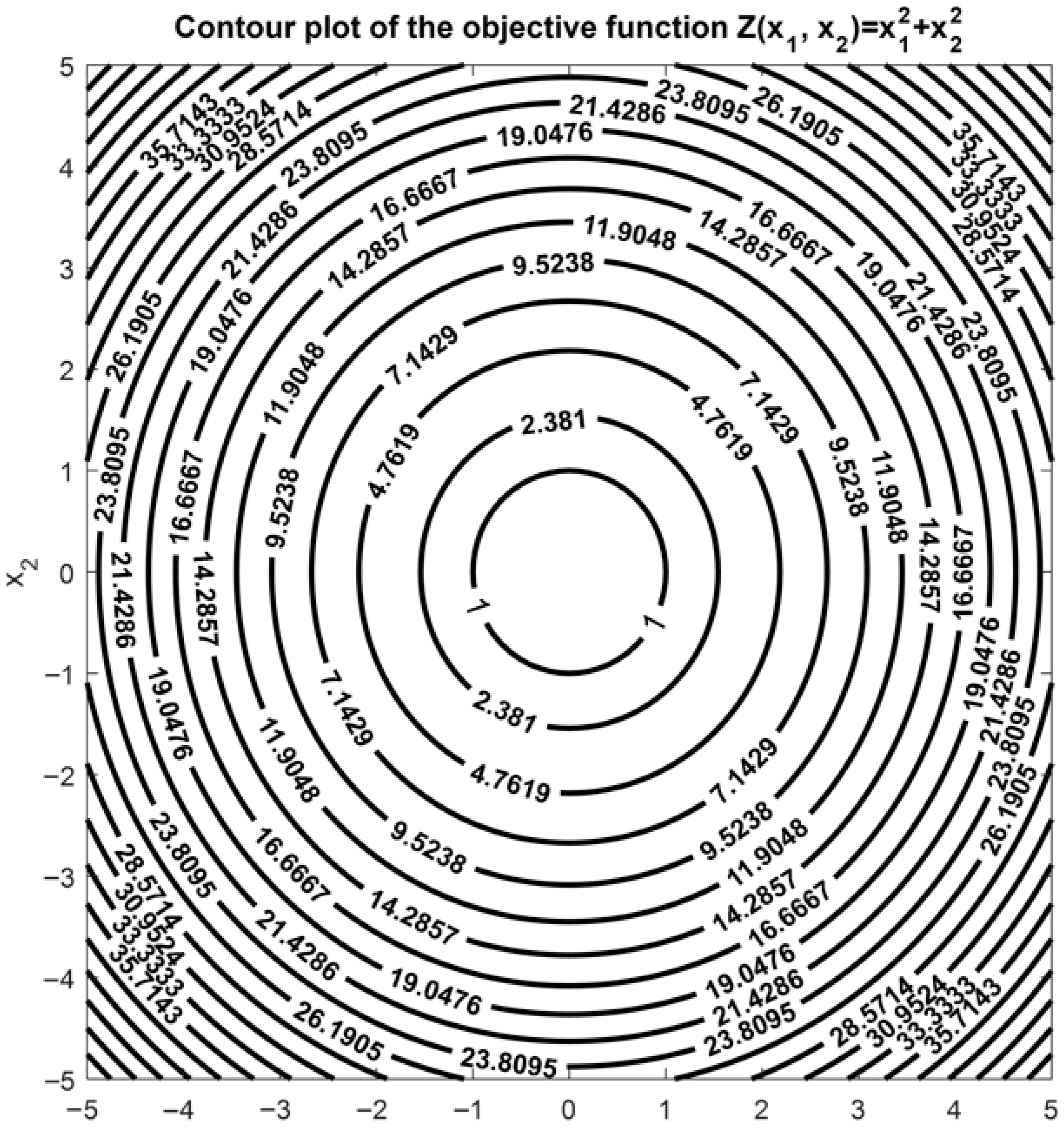
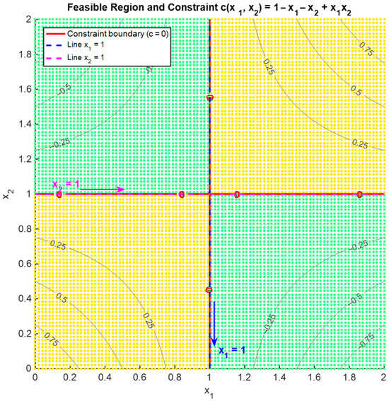
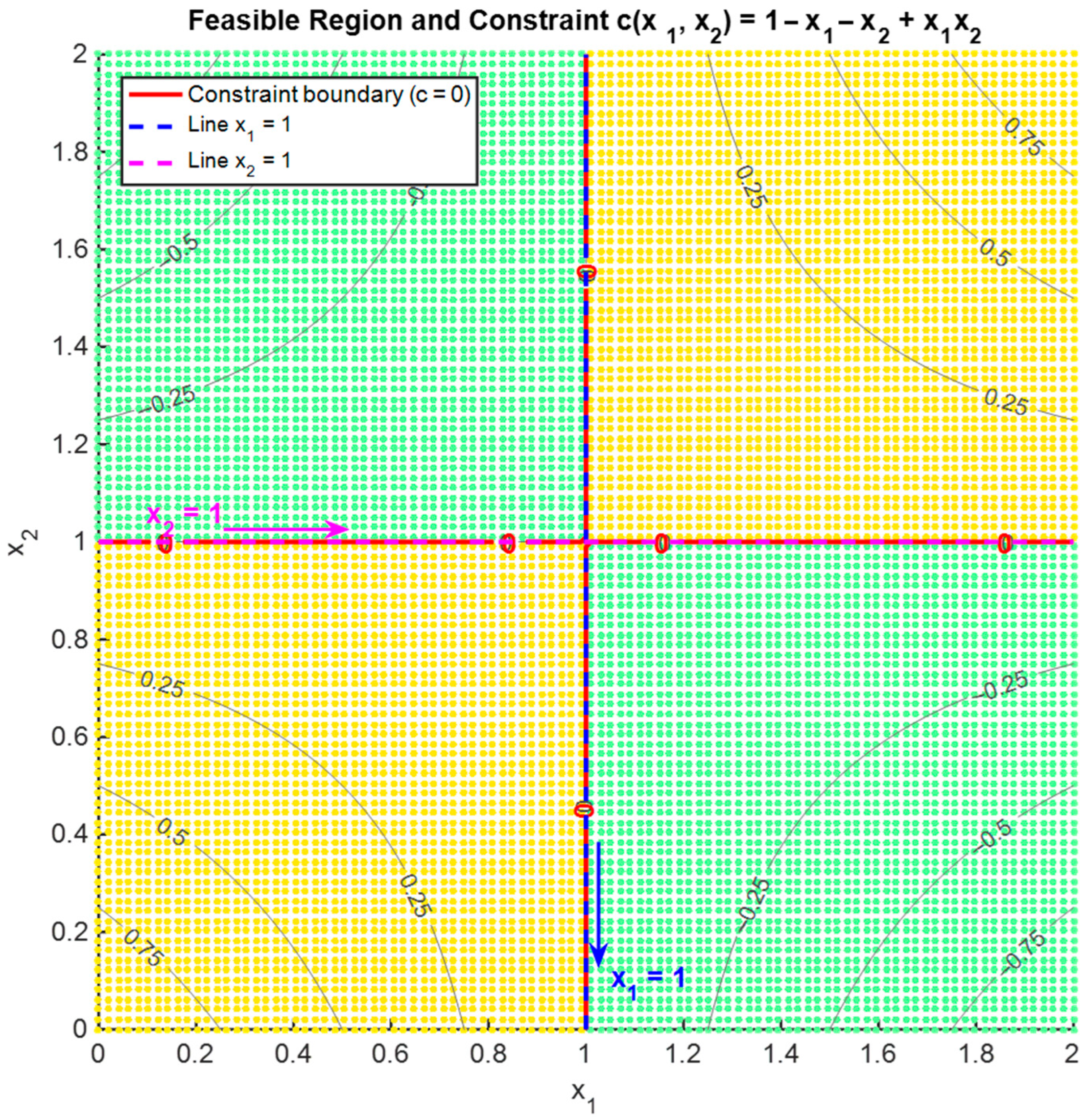
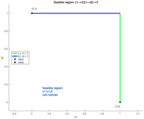
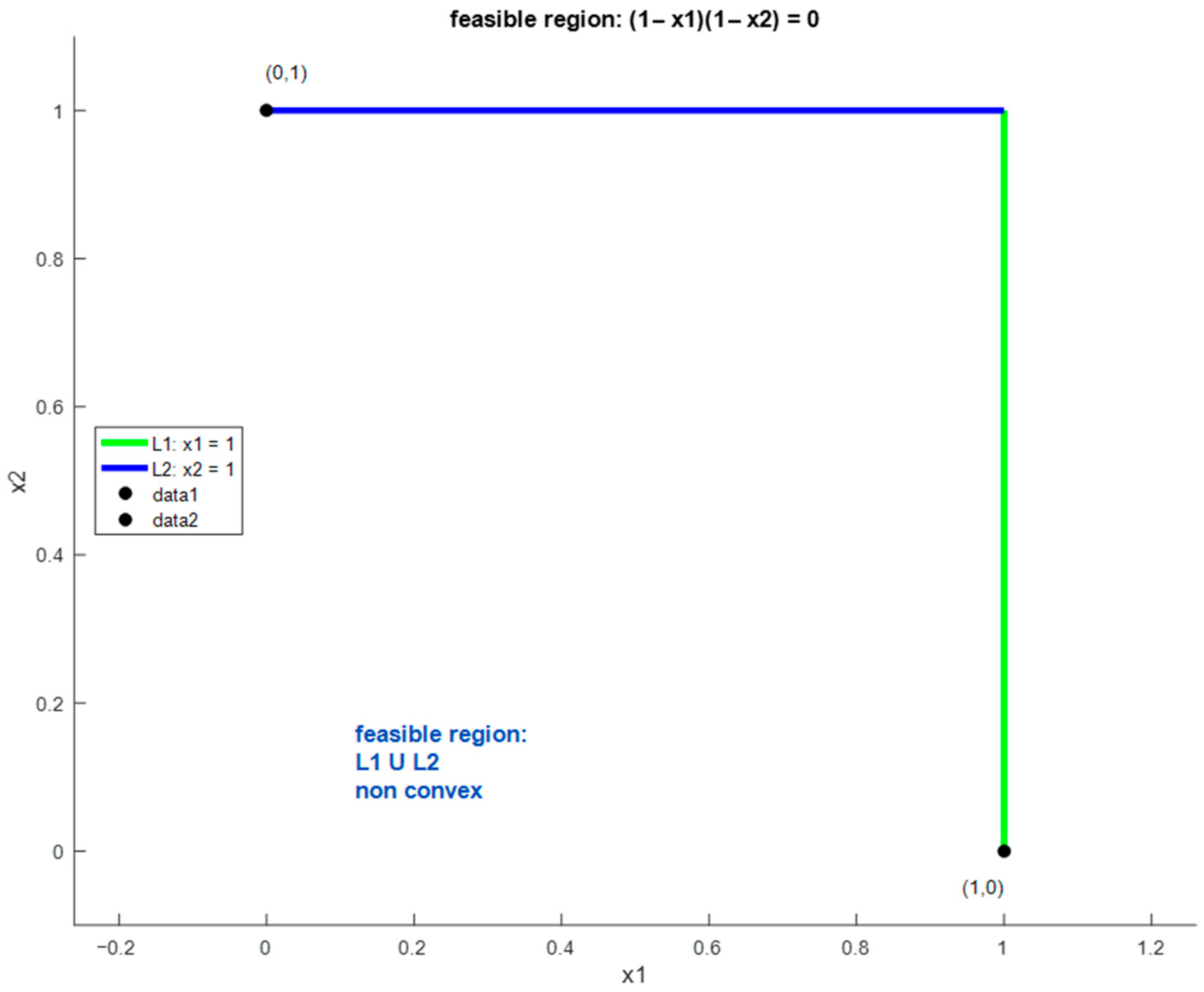
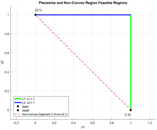
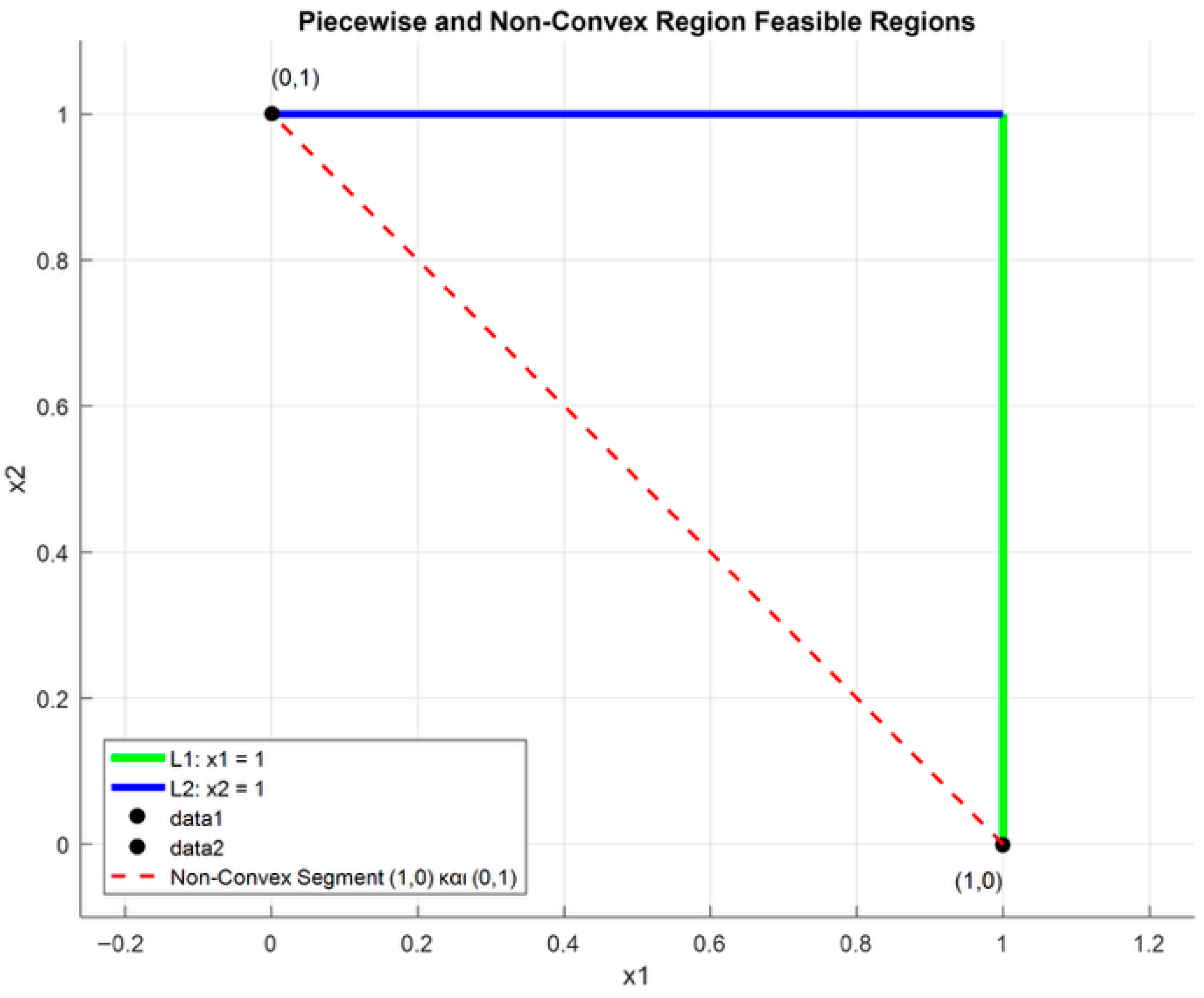
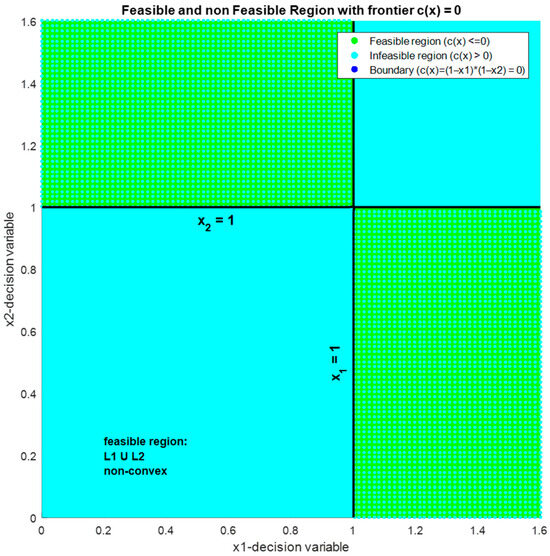
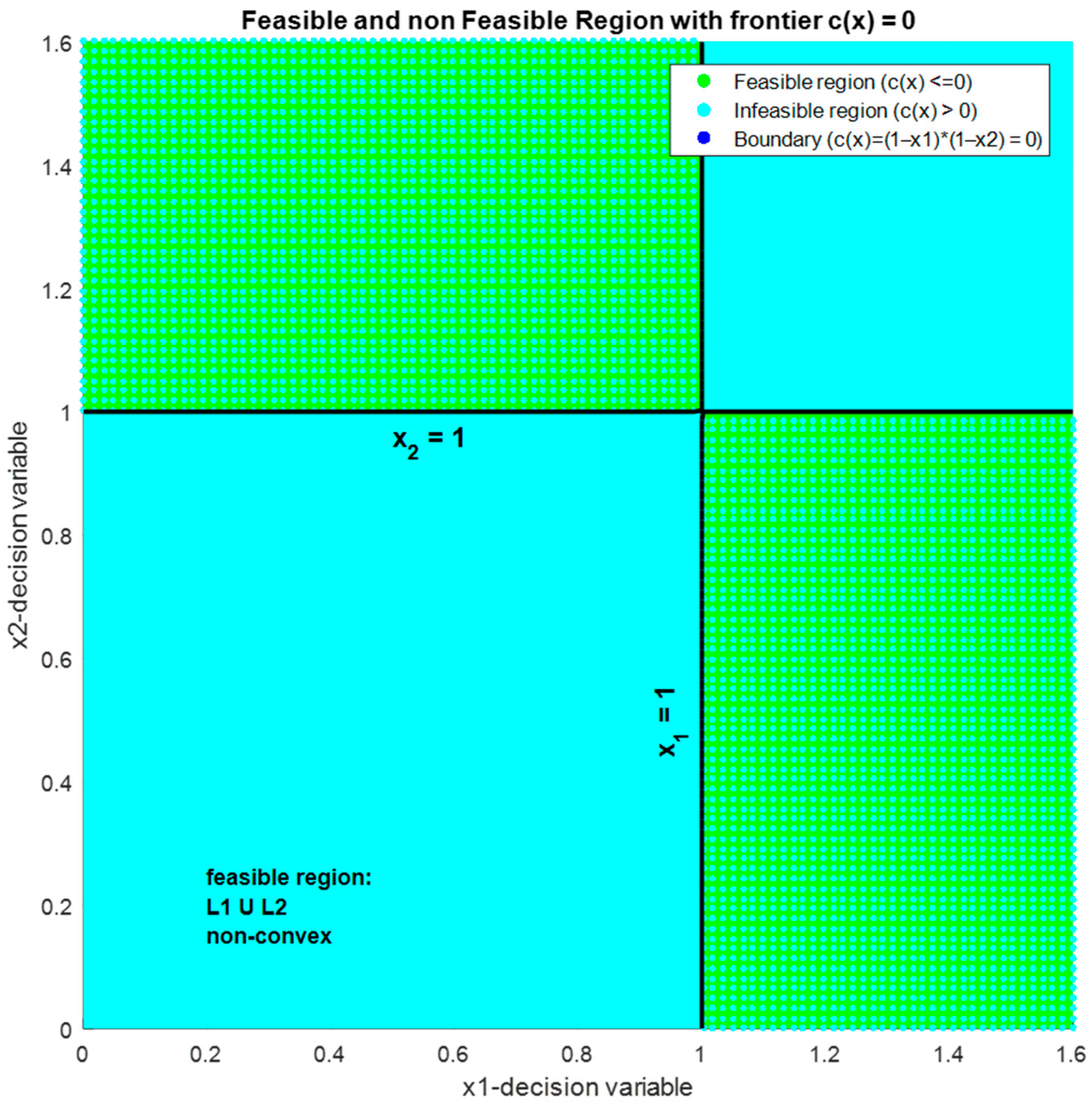
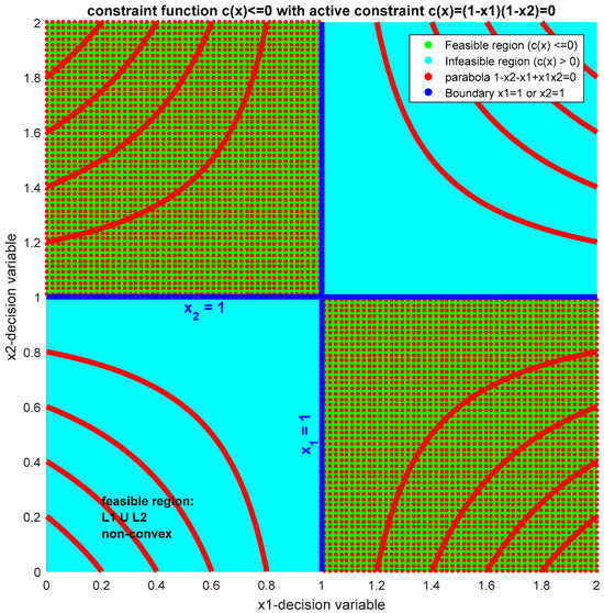
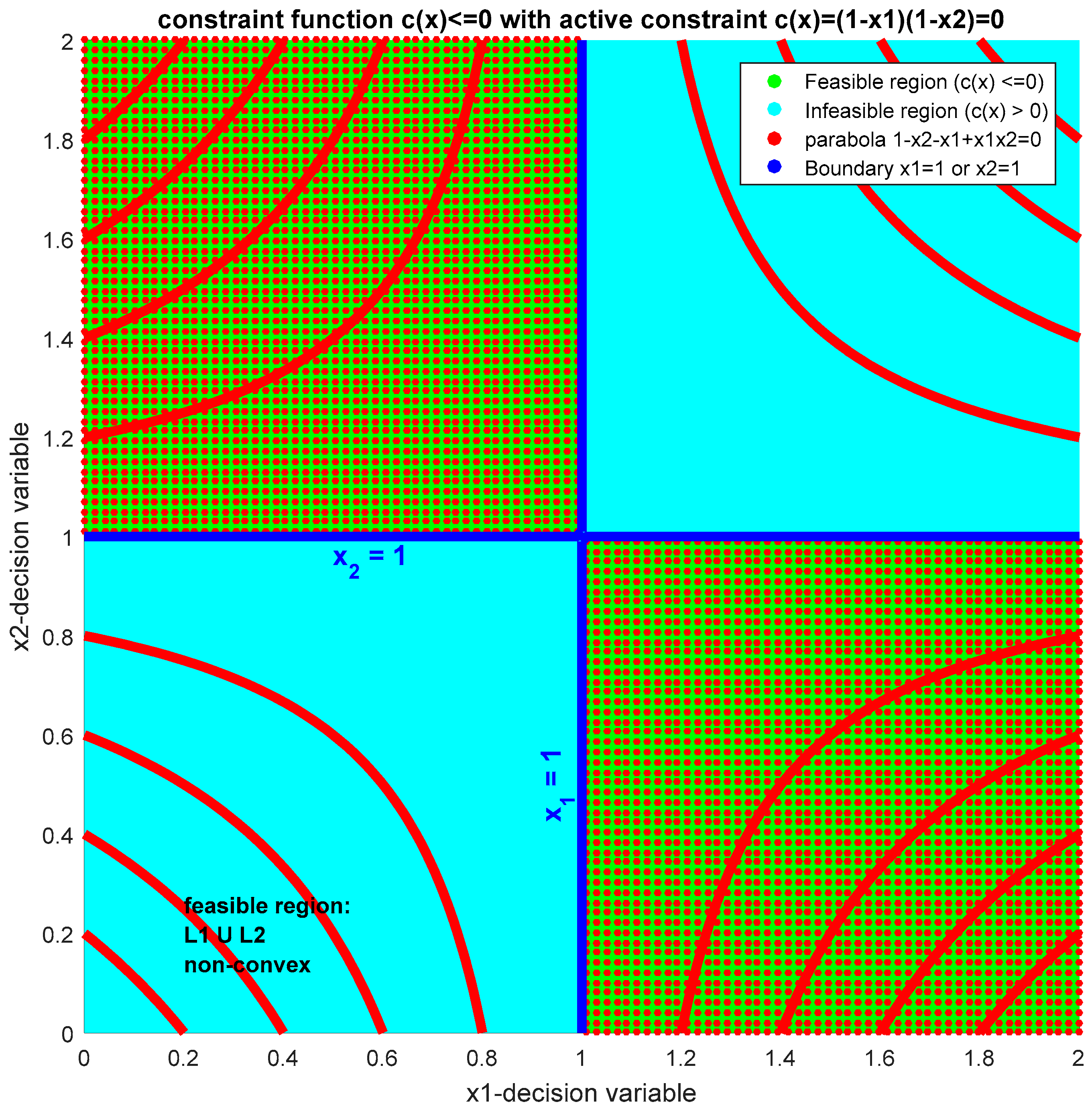
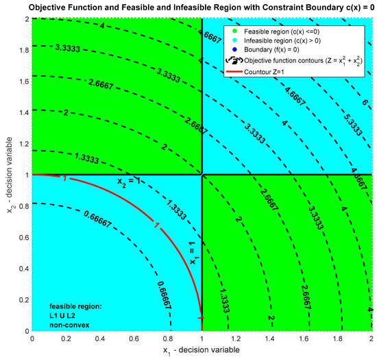
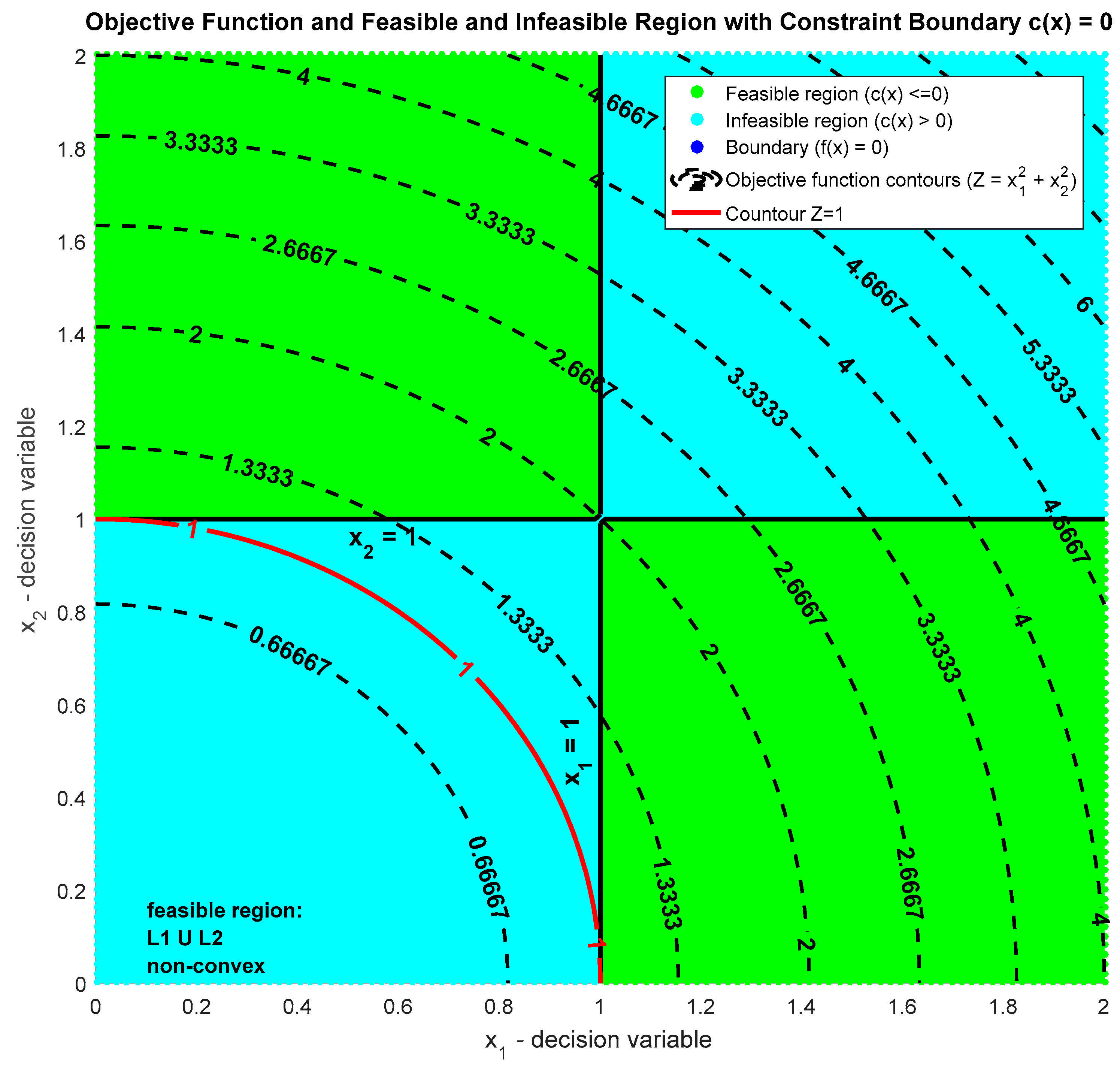
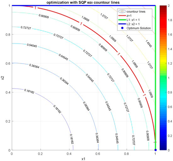
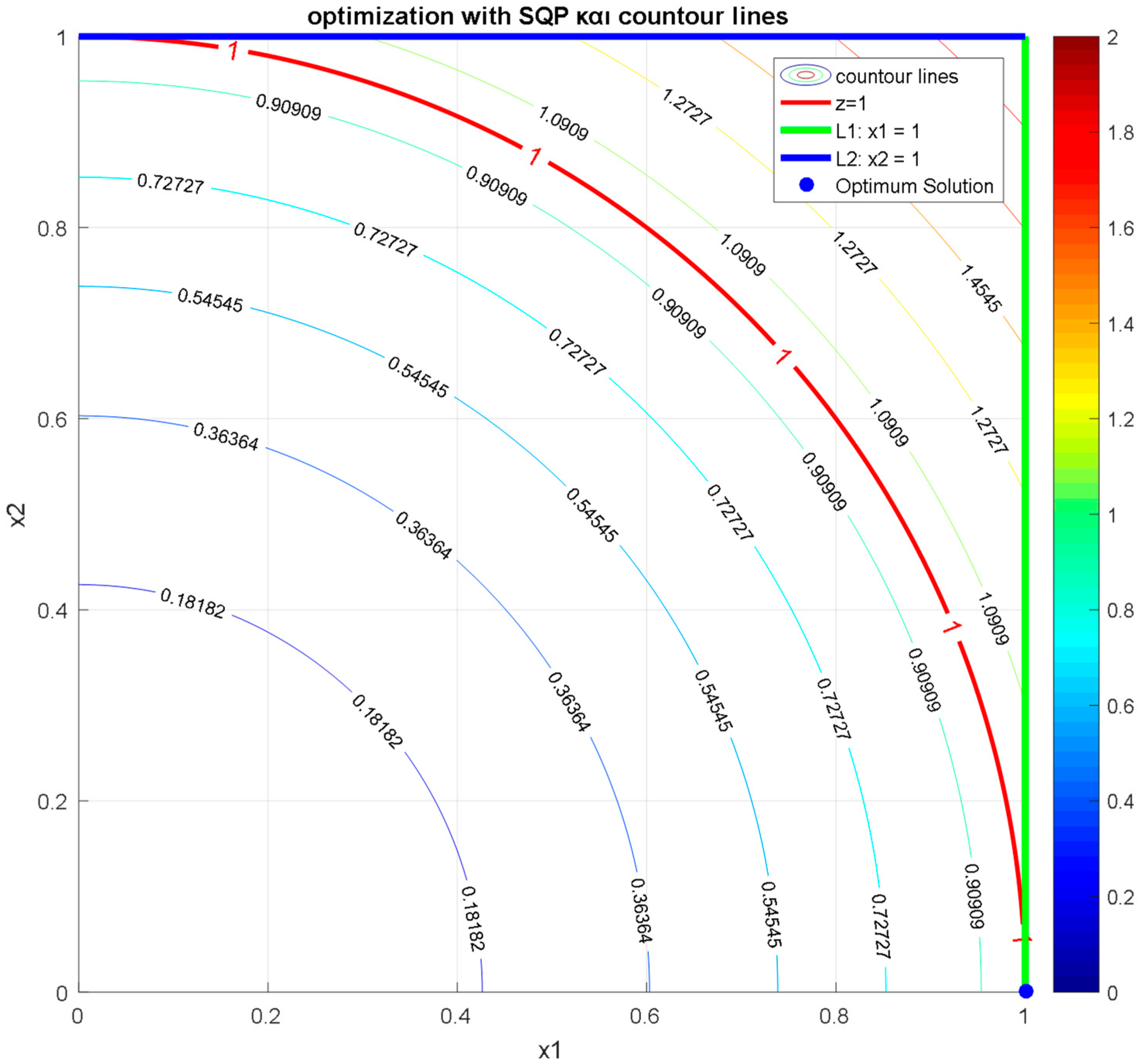
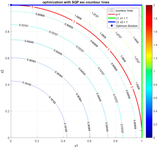
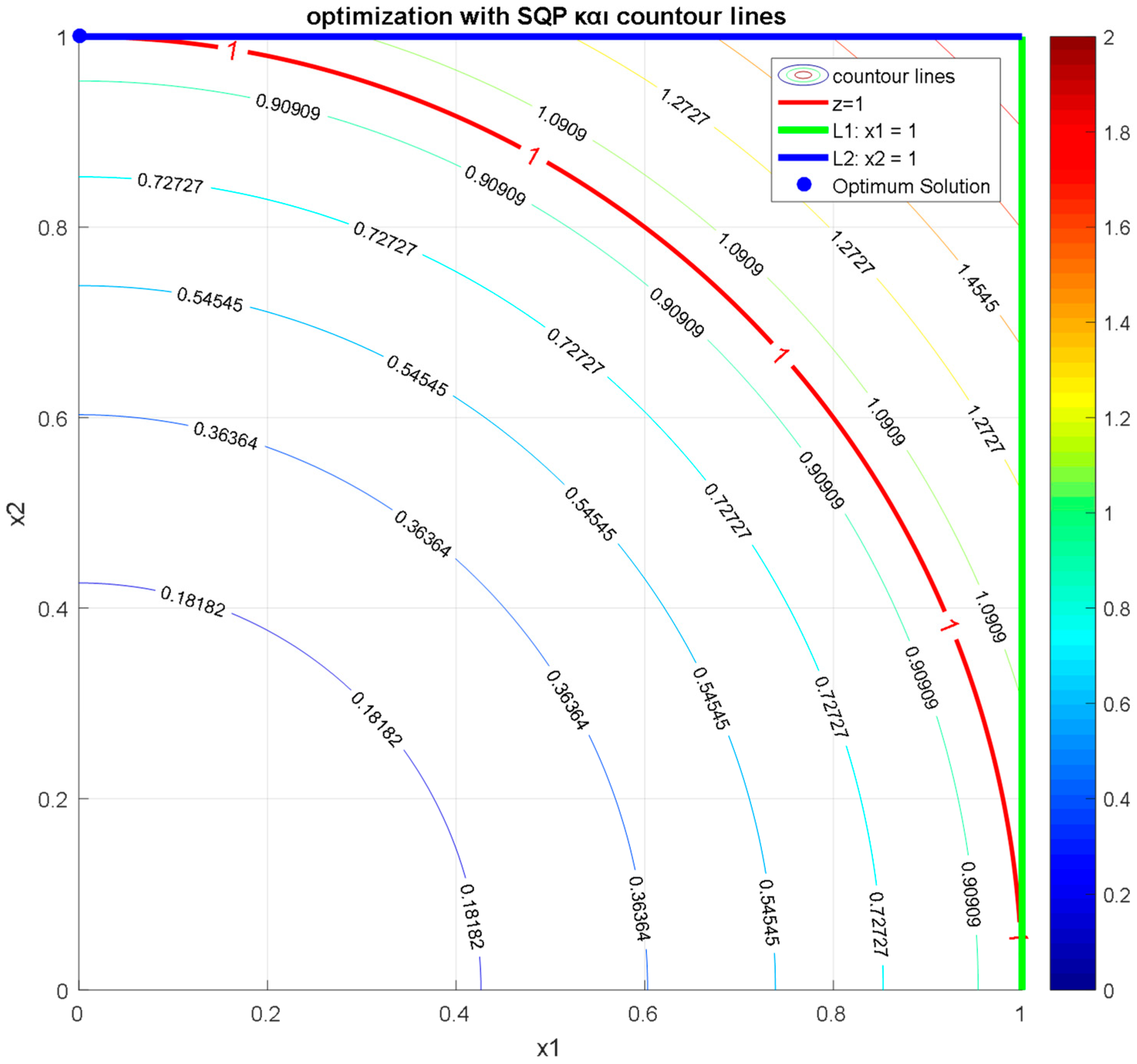
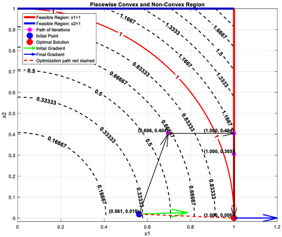
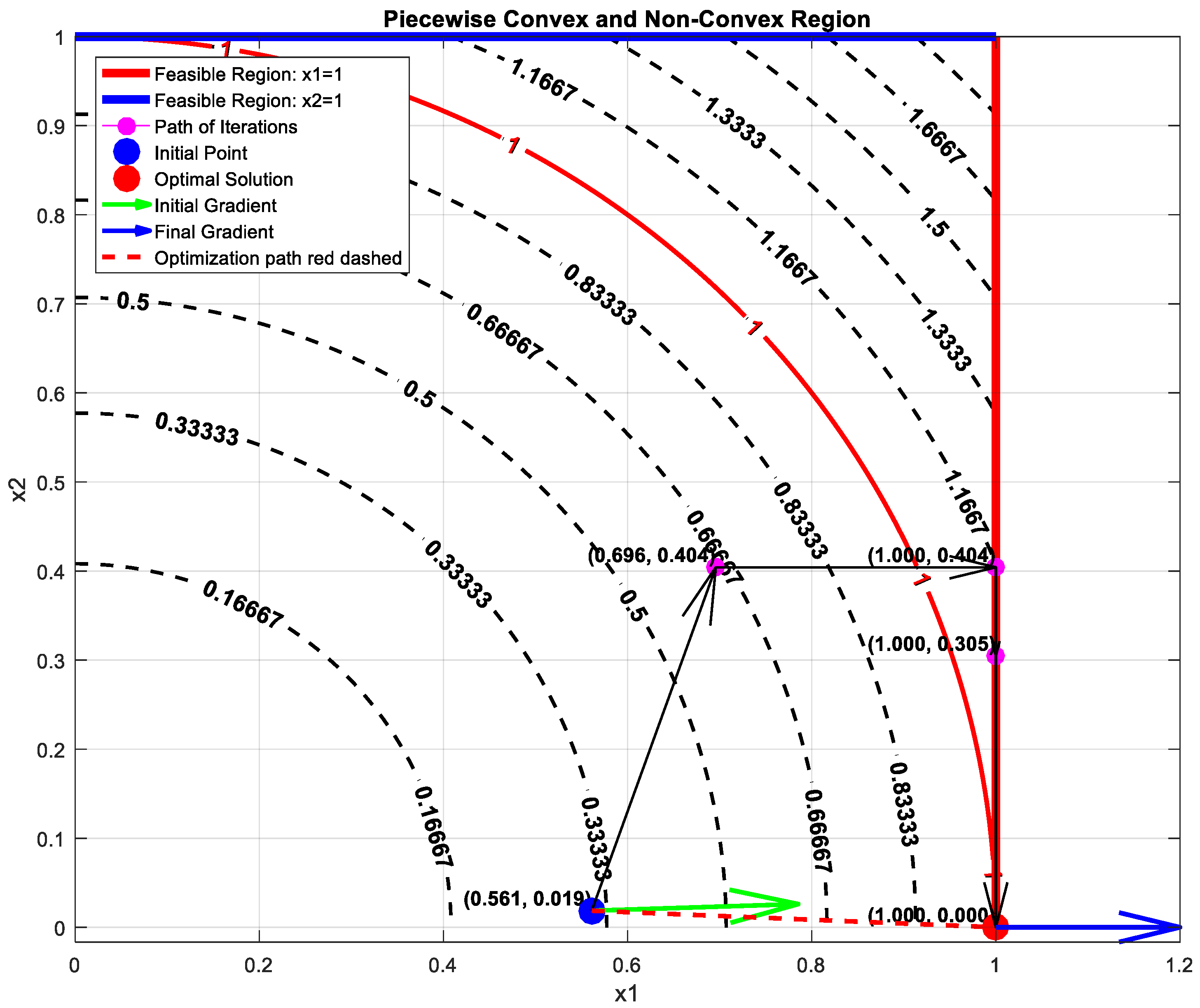
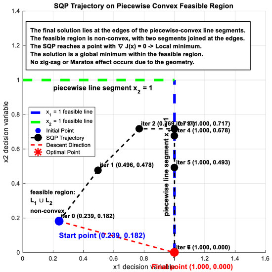
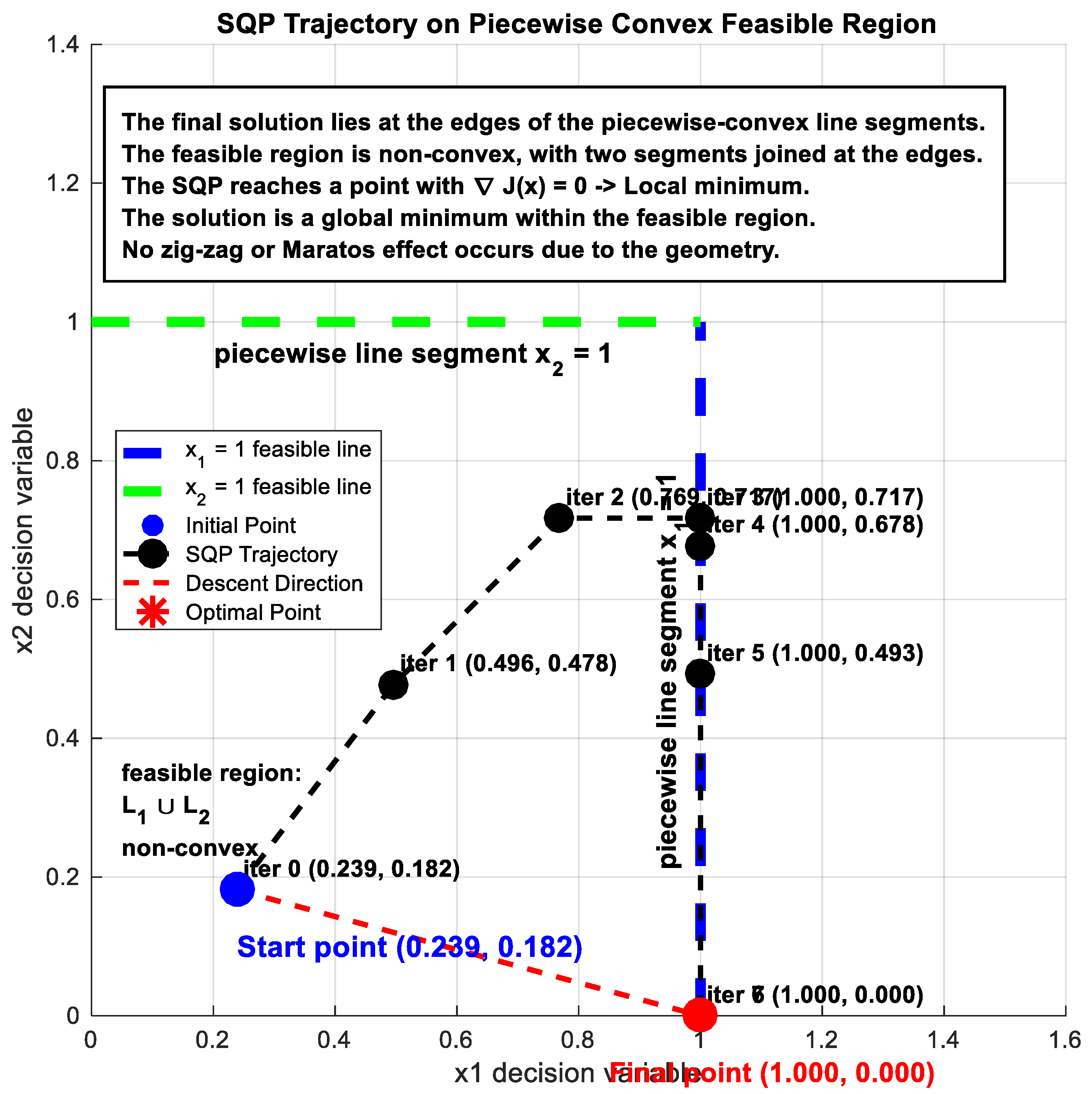
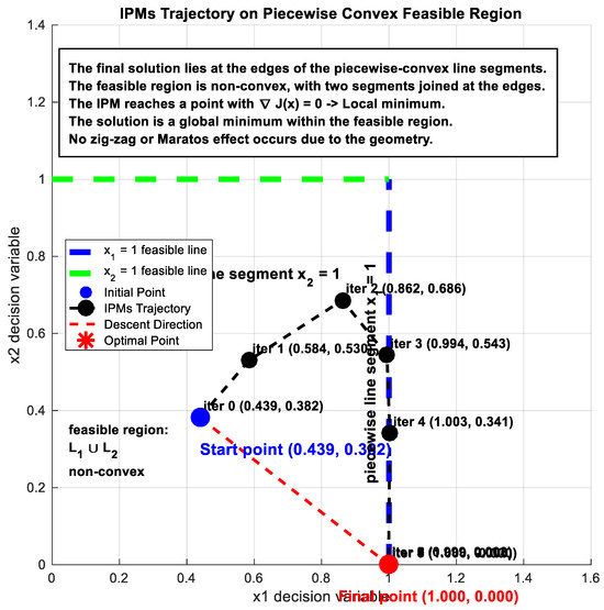
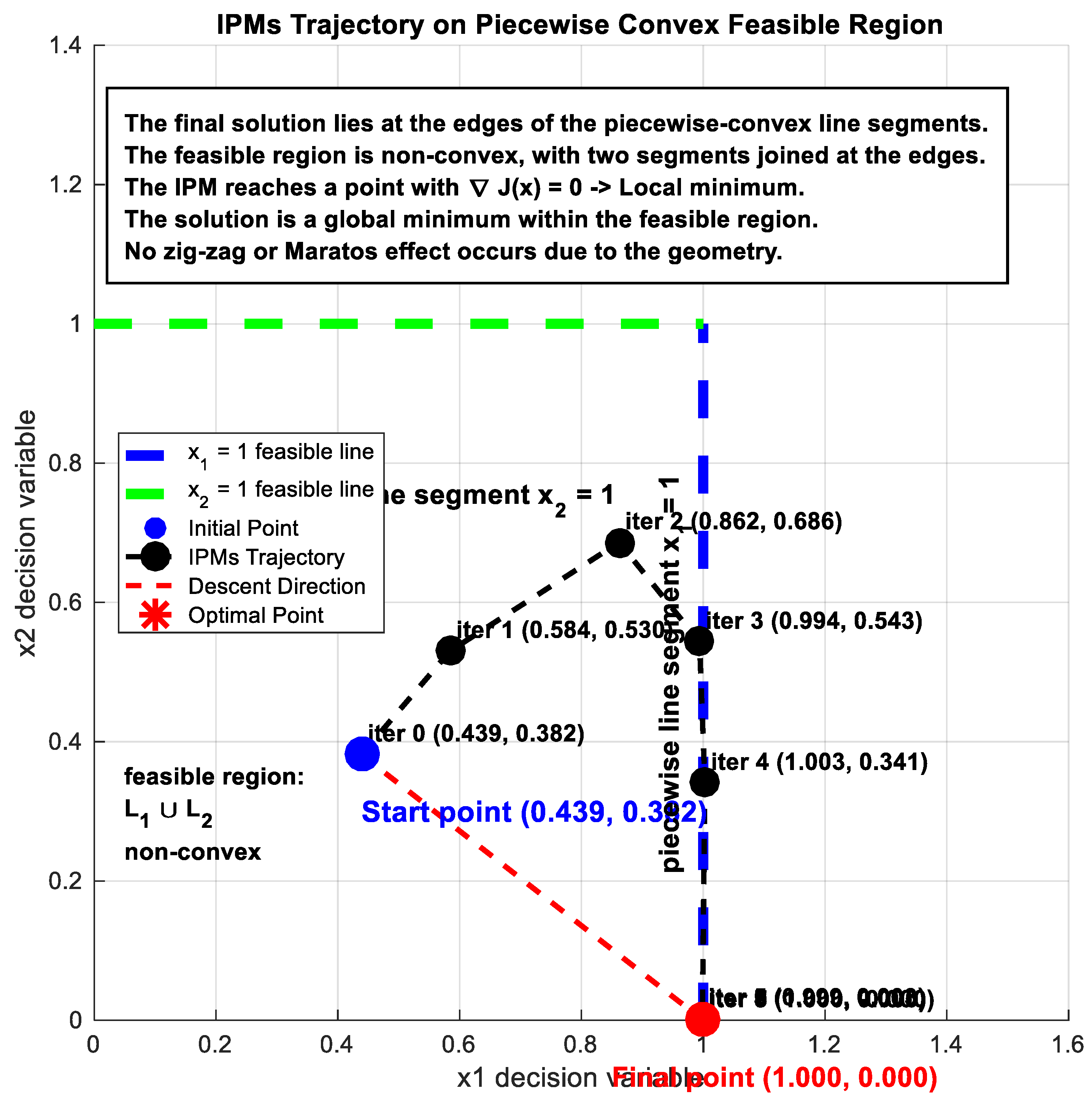
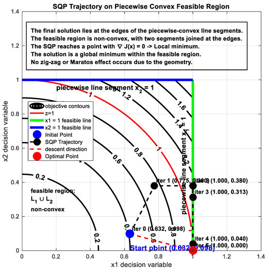
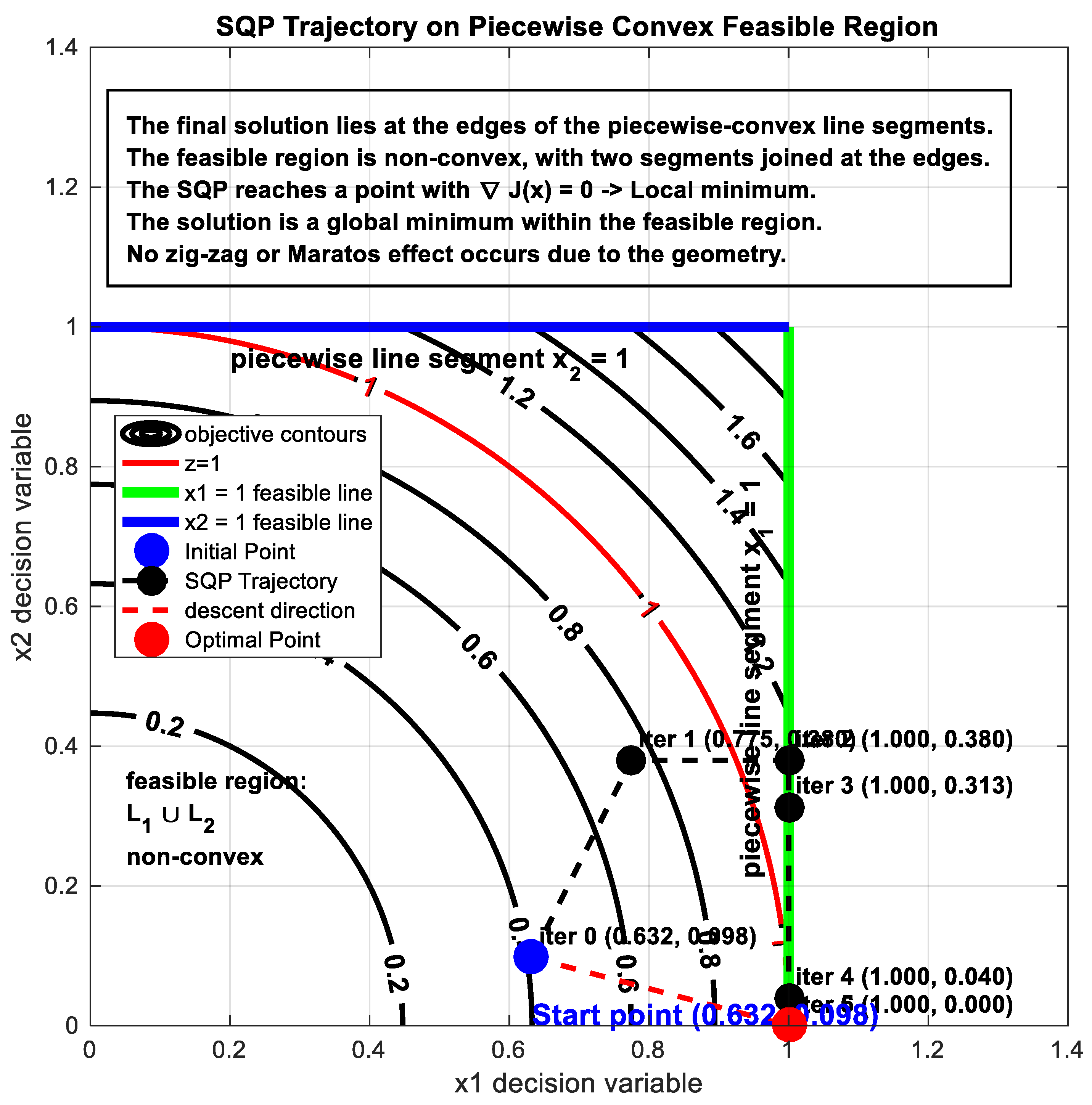
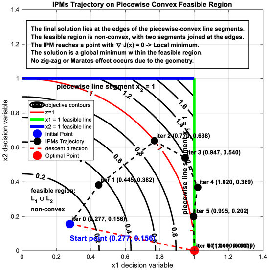
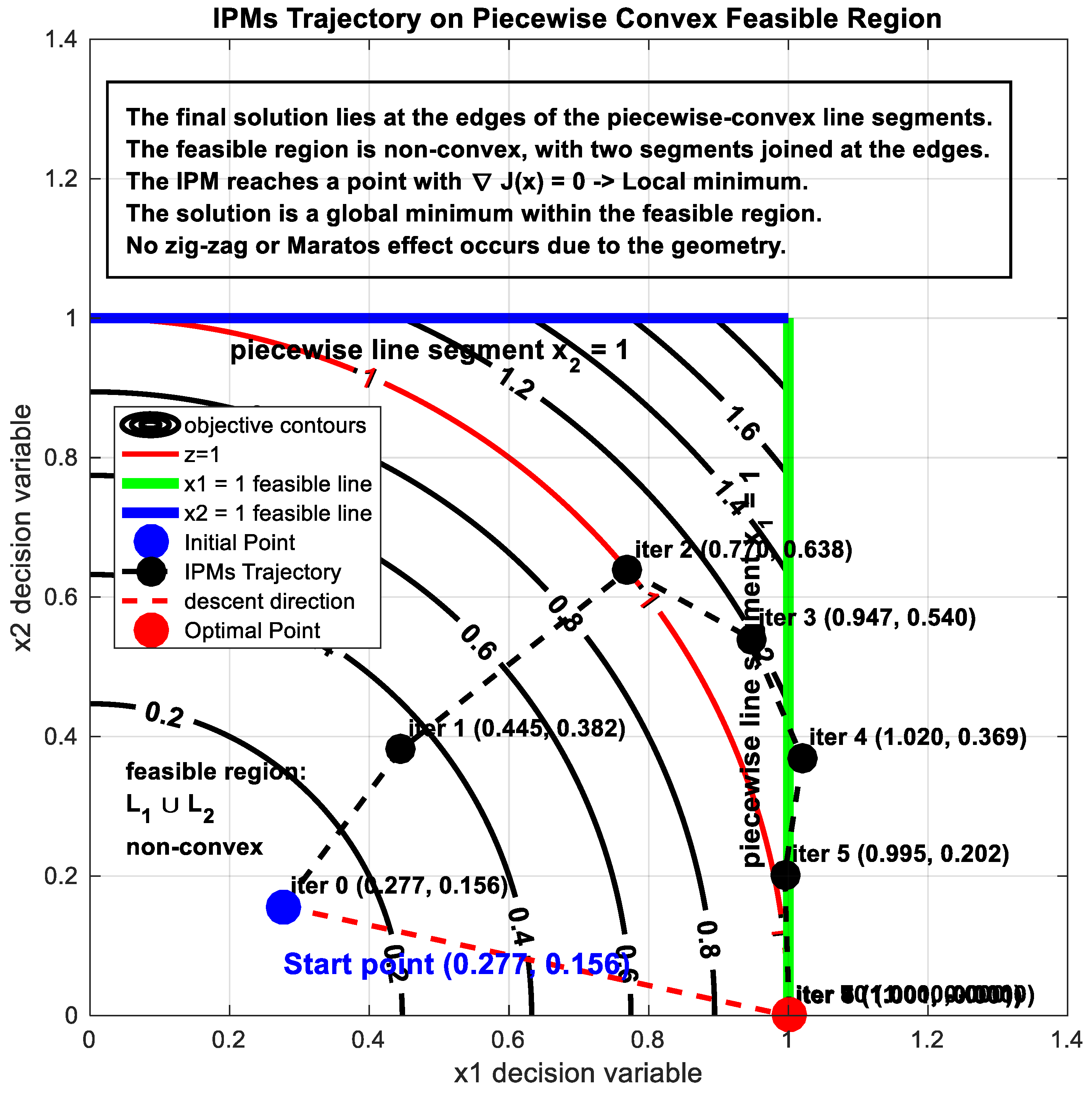
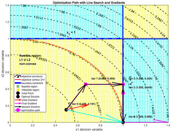
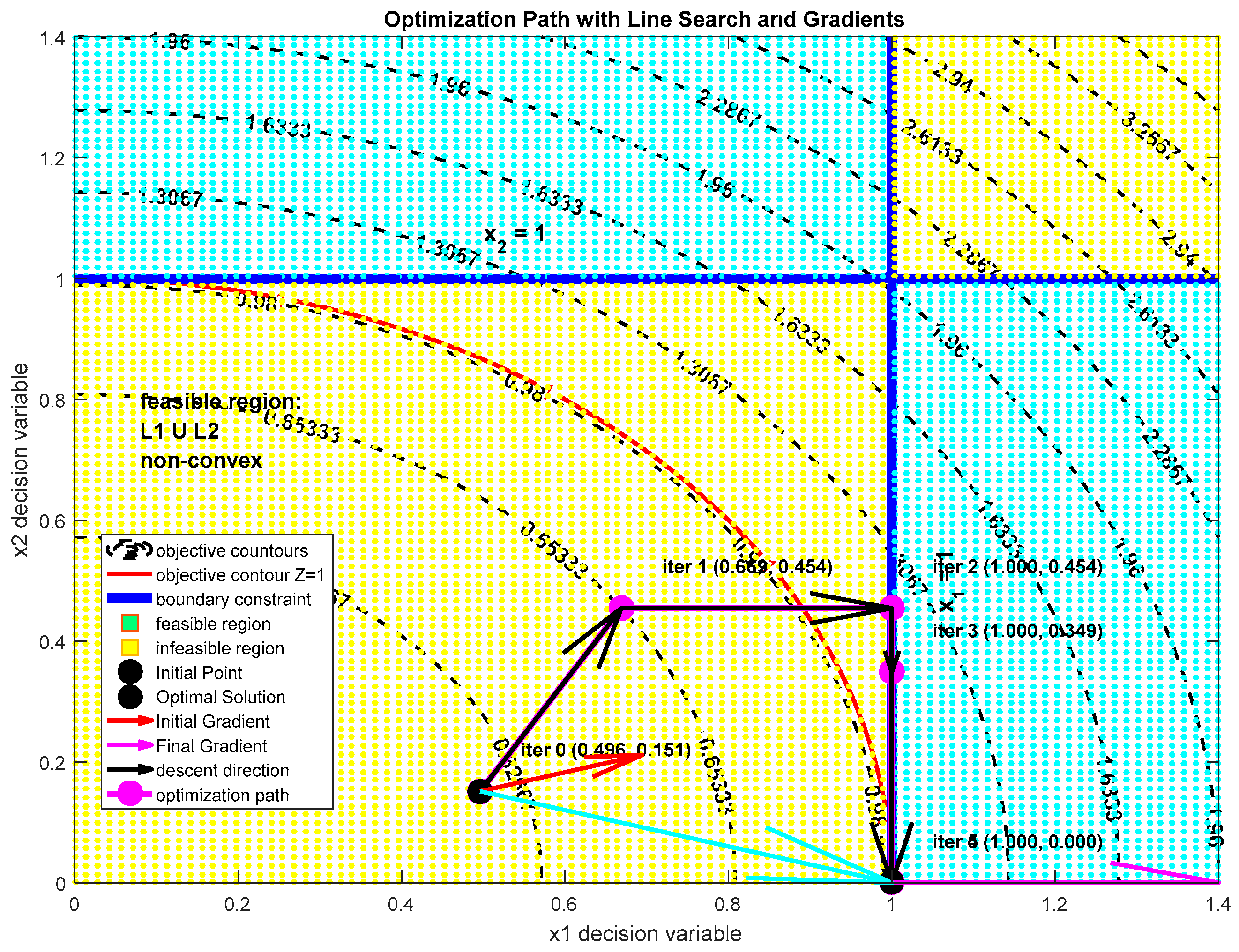
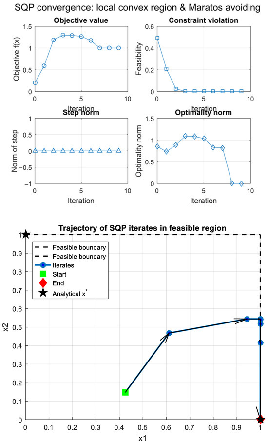
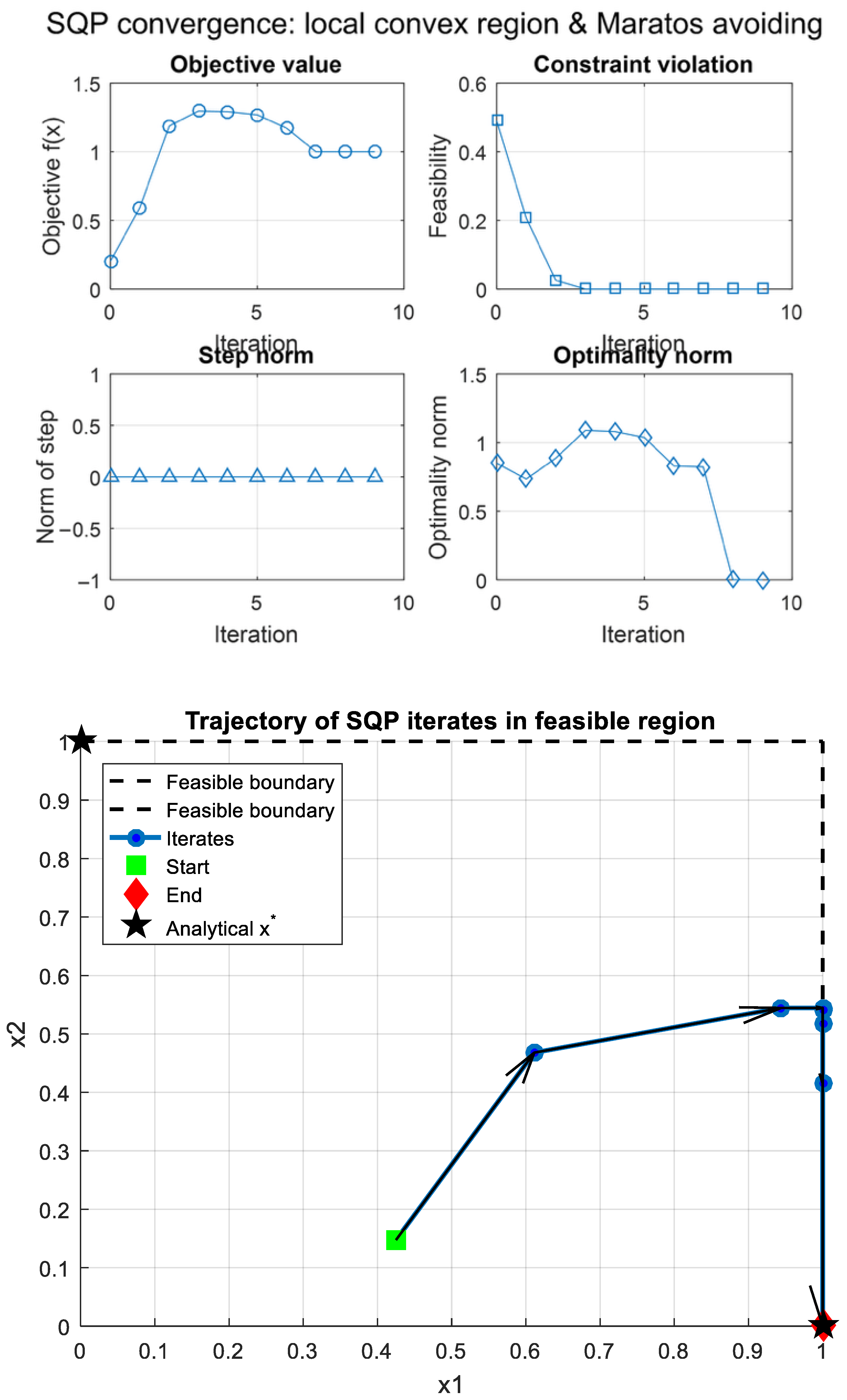
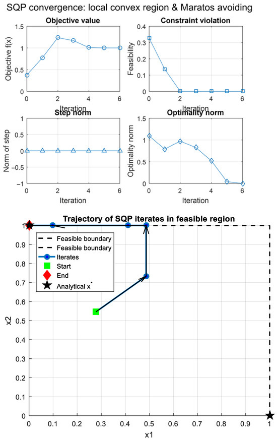
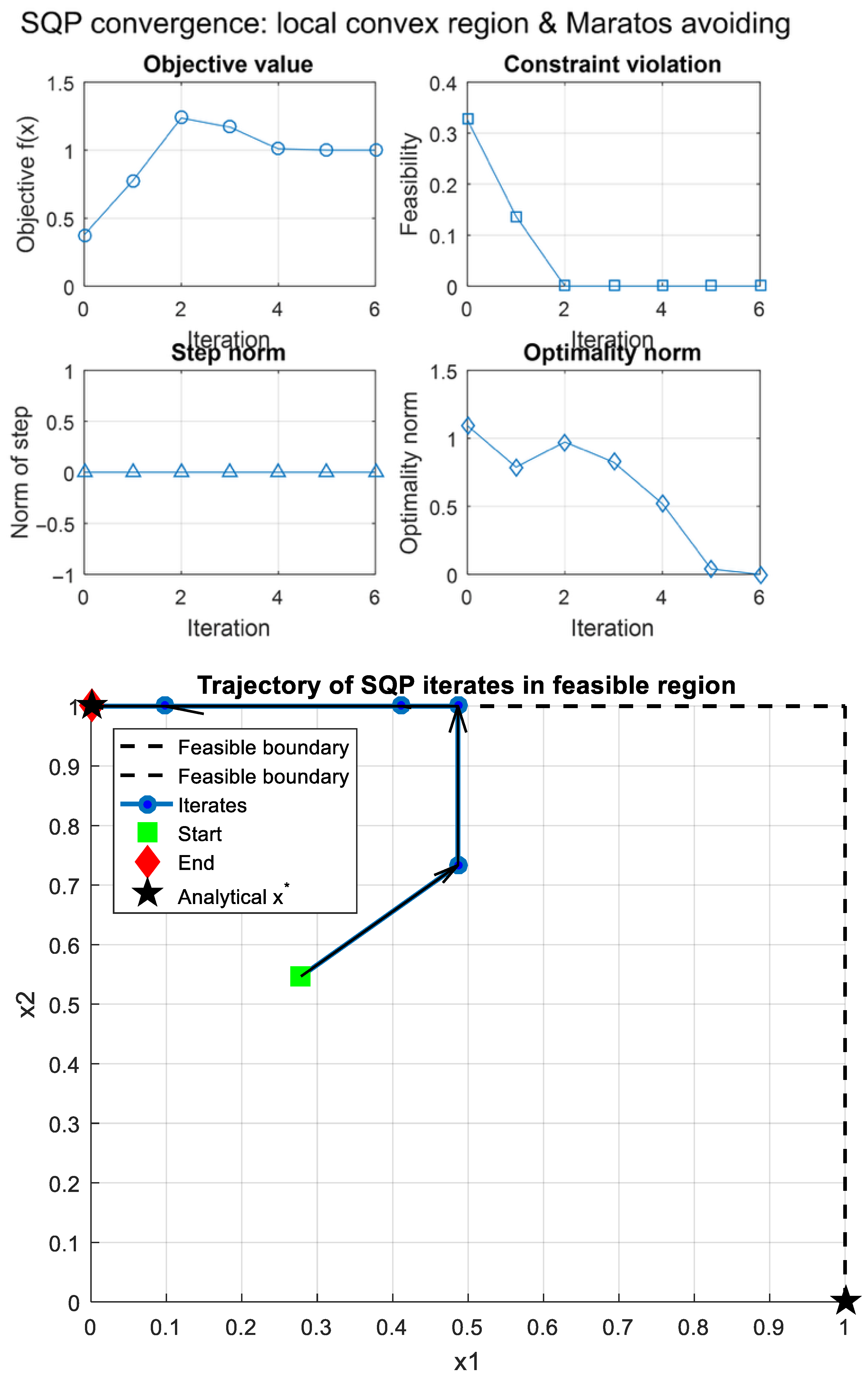

Disclaimer/Publisher’s Note: The statements, opinions and data contained in all publications are solely those of the individual author(s) and contributor(s) and not of MDPI and/or the editor(s). MDPI and/or the editor(s) disclaim responsibility for any injury to people or property resulting from any ideas, methods, instructions or products referred to in the content. |
© 2025 by the authors. Licensee MDPI, Basel, Switzerland. This article is an open access article distributed under the terms and conditions of the Creative Commons Attribution (CC BY) license.