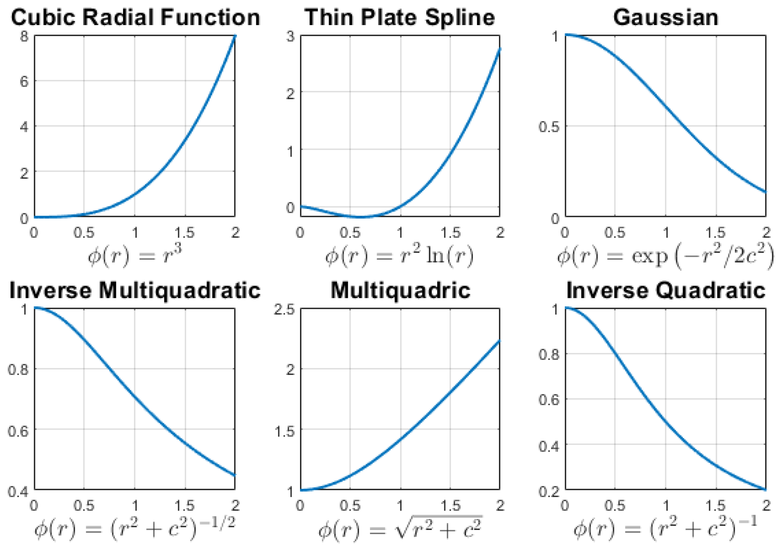
Figure 1.
Radial basis functions (RBFs) plotted with shape parameter . Gaussian, multiquadric, and inverse multiquadric RBFs exhibit different decay and smoothness behaviors. Polynomial-based functions like cubic and thin plate spline do not depend on c. The choice of RBF affects interpolation accuracy and numerical stability.
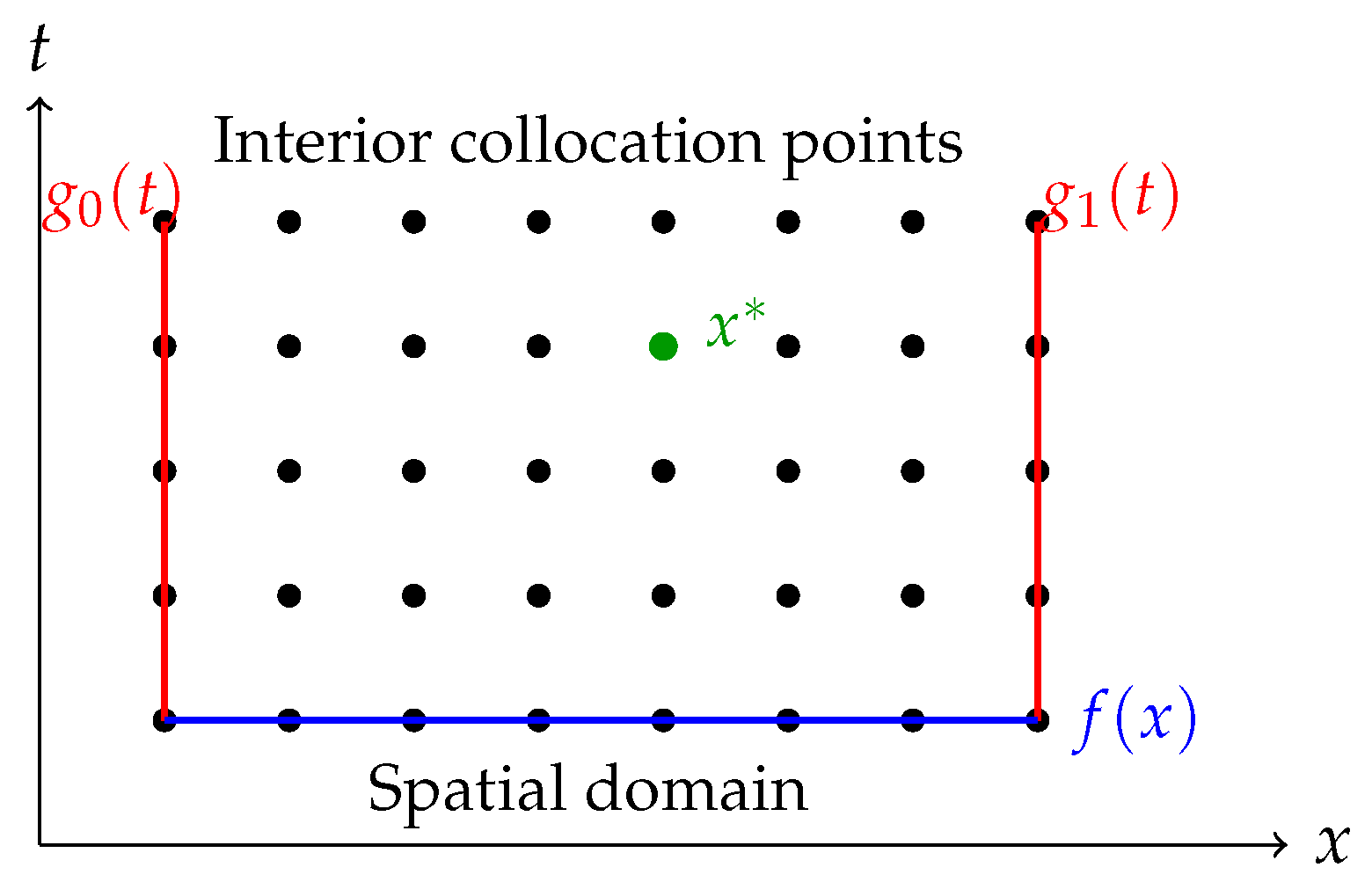
Figure 2.
Space–time grid illustrating the application of conditions in the RBF collocation method. The red edges denote boundary conditions, the bottom edge represents the initial condition, and the green dot marks the interior point where the energy measurement is specified.
Figure 2.
Space–time grid illustrating the application of conditions in the RBF collocation method. The red edges denote boundary conditions, the bottom edge represents the initial condition, and the green dot marks the interior point where the energy measurement is specified.
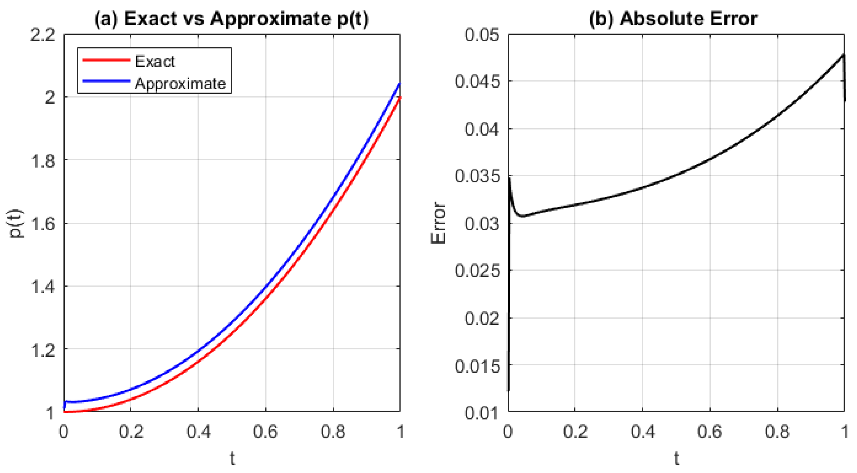
Figure 3.
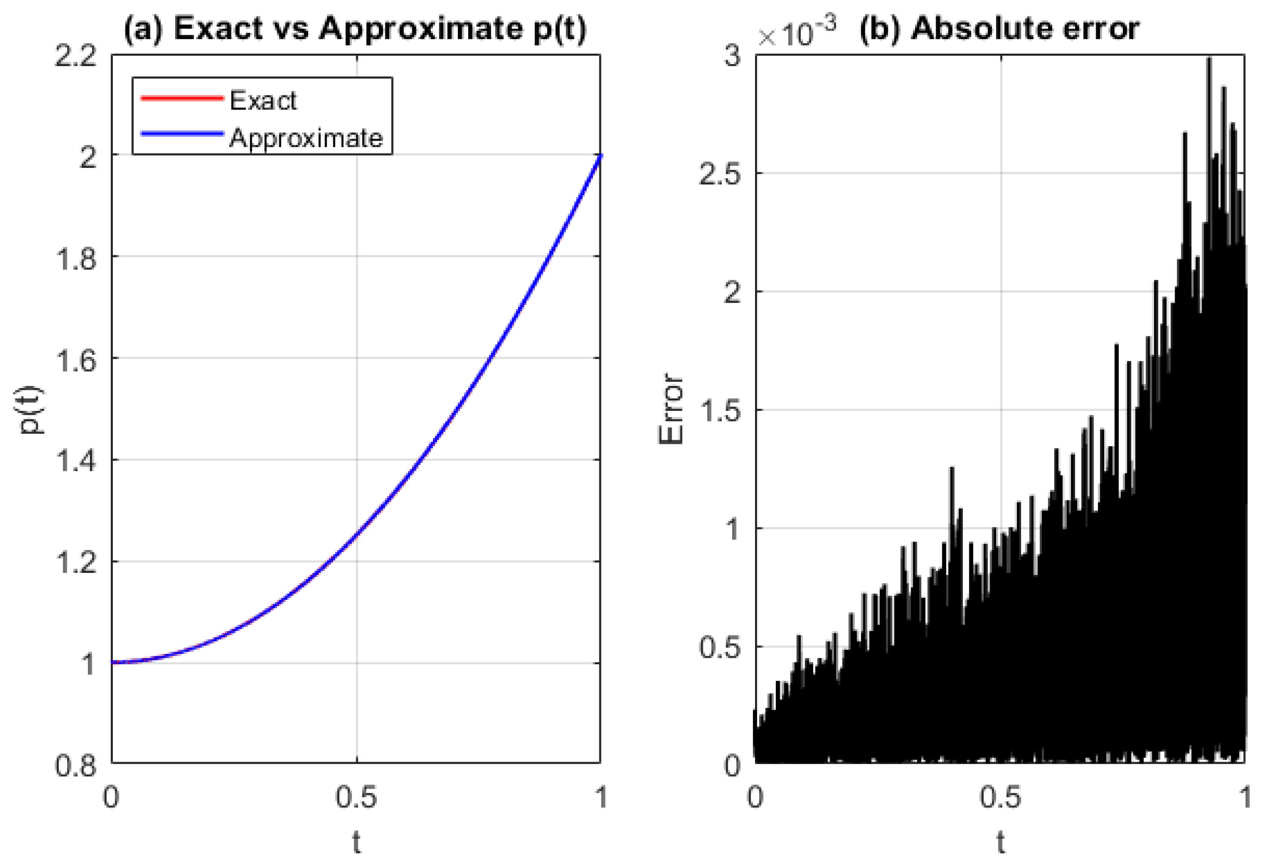
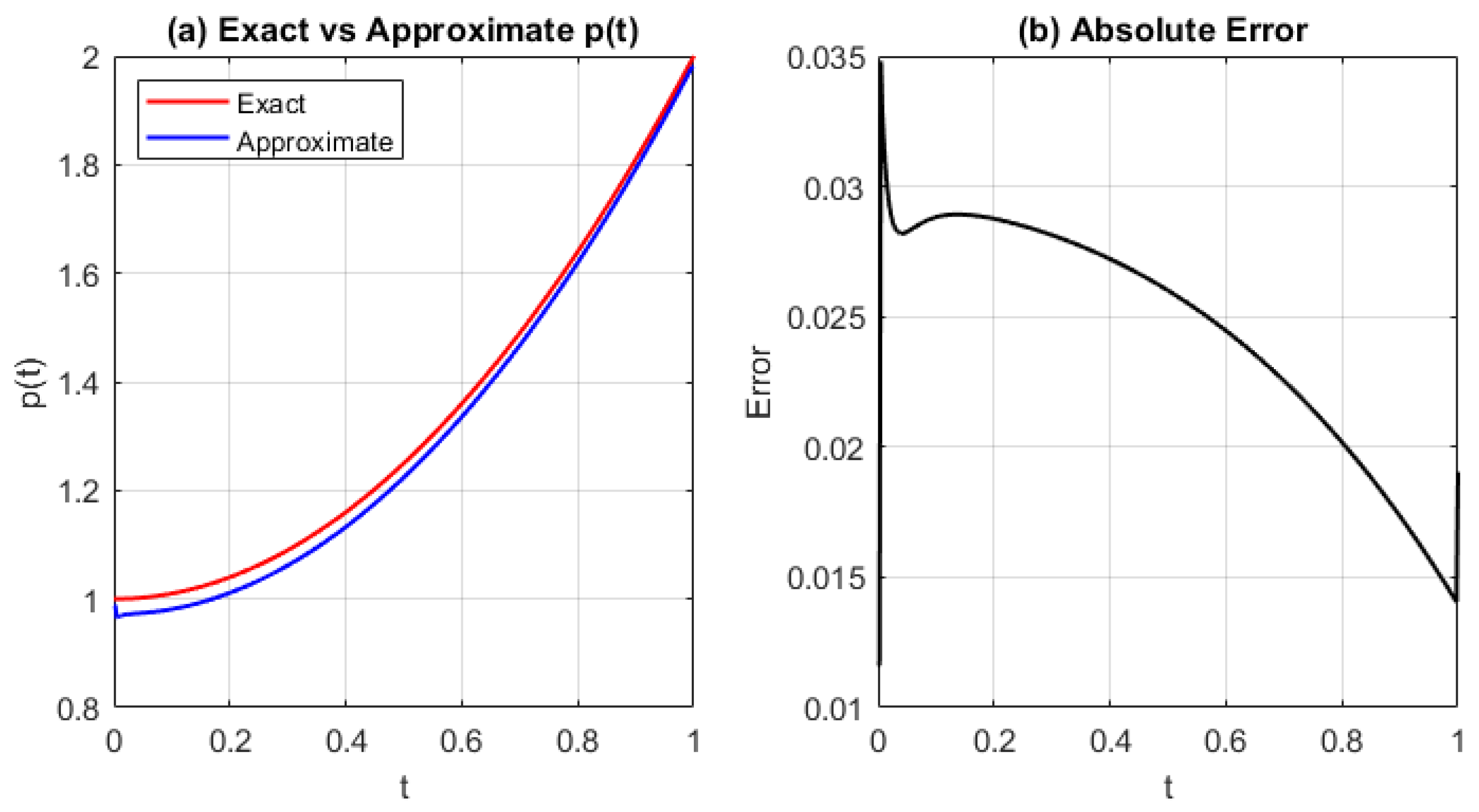
(a) Exact vs approximated source function , and (b) absolute error using GRBF with and . The initial error is high and increases linearly with t, indicating acceptable convergence behavior.
Figure 3.
(a) Exact vs approximated source function , and (b) absolute error using GRBF with and . The initial error is high and increases linearly with t, indicating acceptable convergence behavior.
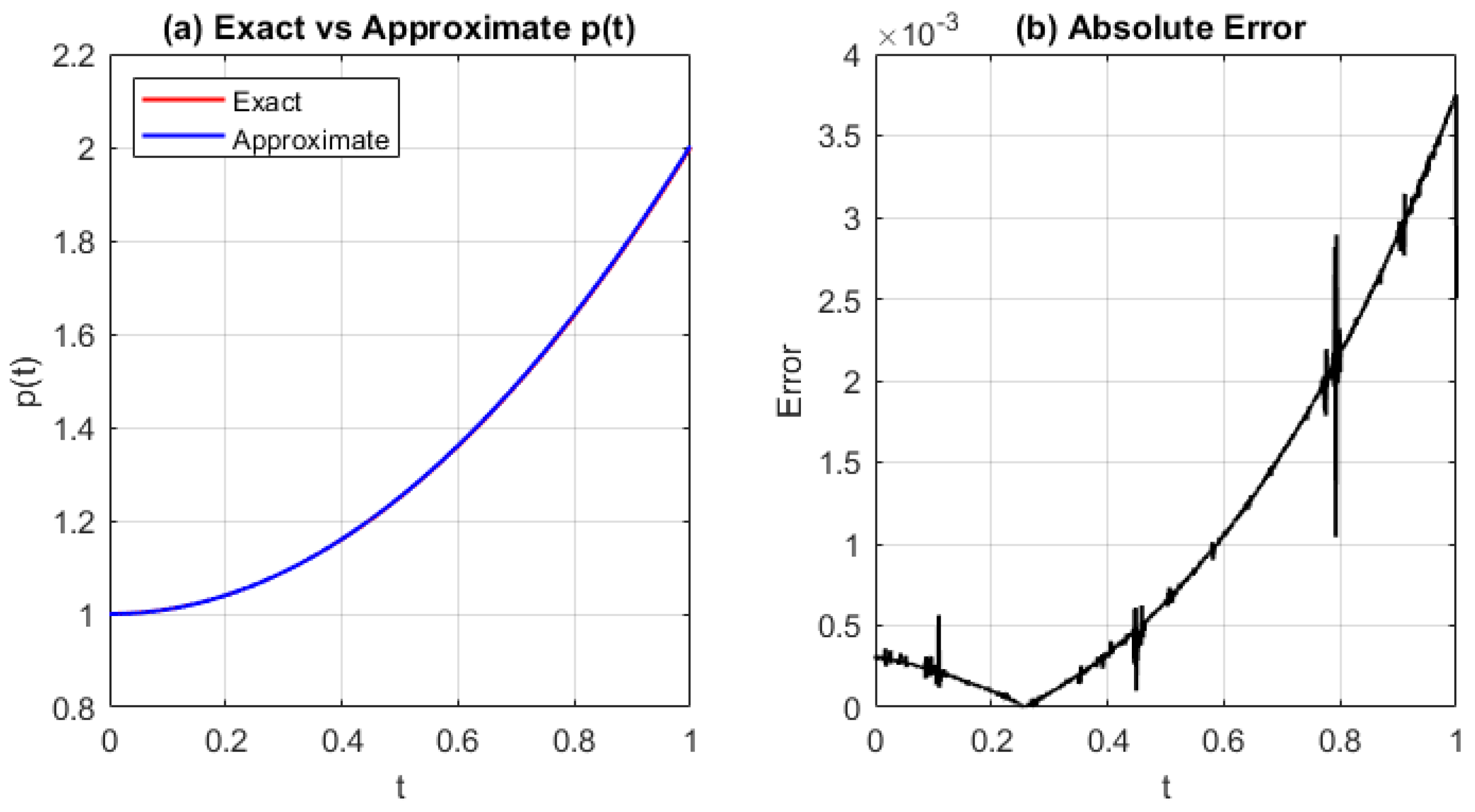
Figure 4.
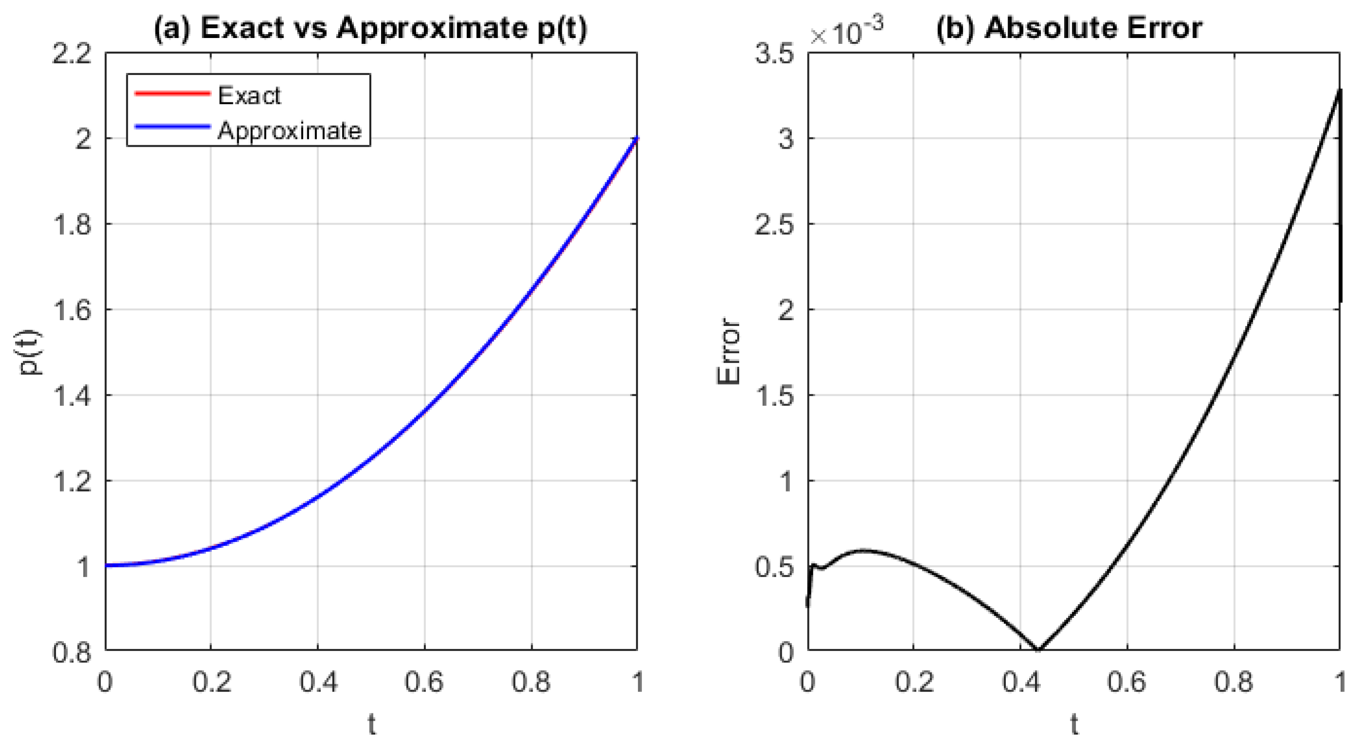
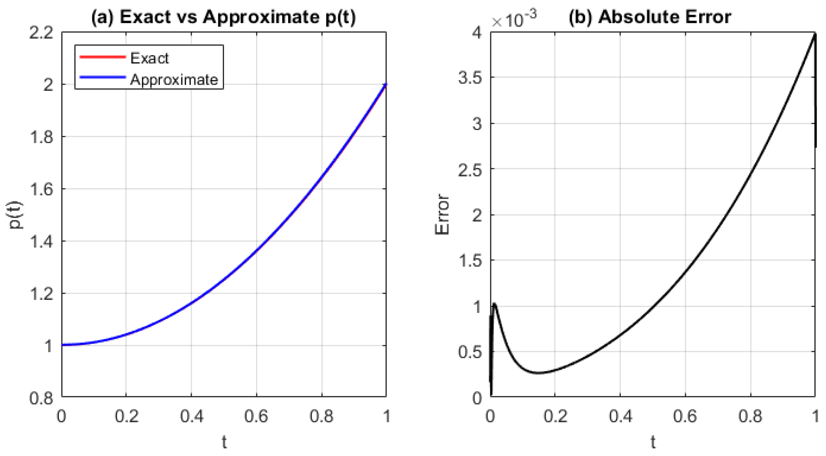
(
a) Exact and approximated source function
, and (
b) absolute error
using the GRBF with refined grid (
) and shape parameter
. The error magnitude is reduced compared to coarser discretization (
Figure 3), demonstrating the benefit of mesh refinement for accuracy.
Figure 4.
(
a) Exact and approximated source function
, and (
b) absolute error
using the GRBF with refined grid (
) and shape parameter
. The error magnitude is reduced compared to coarser discretization (
Figure 3), demonstrating the benefit of mesh refinement for accuracy.
Figure 5.
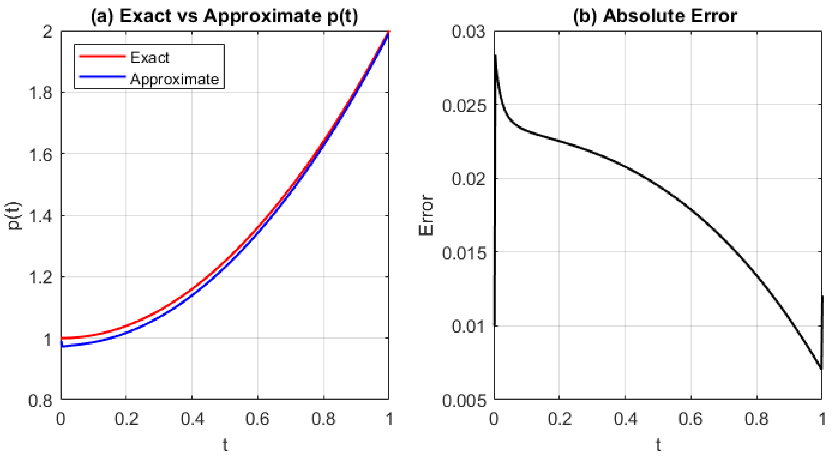
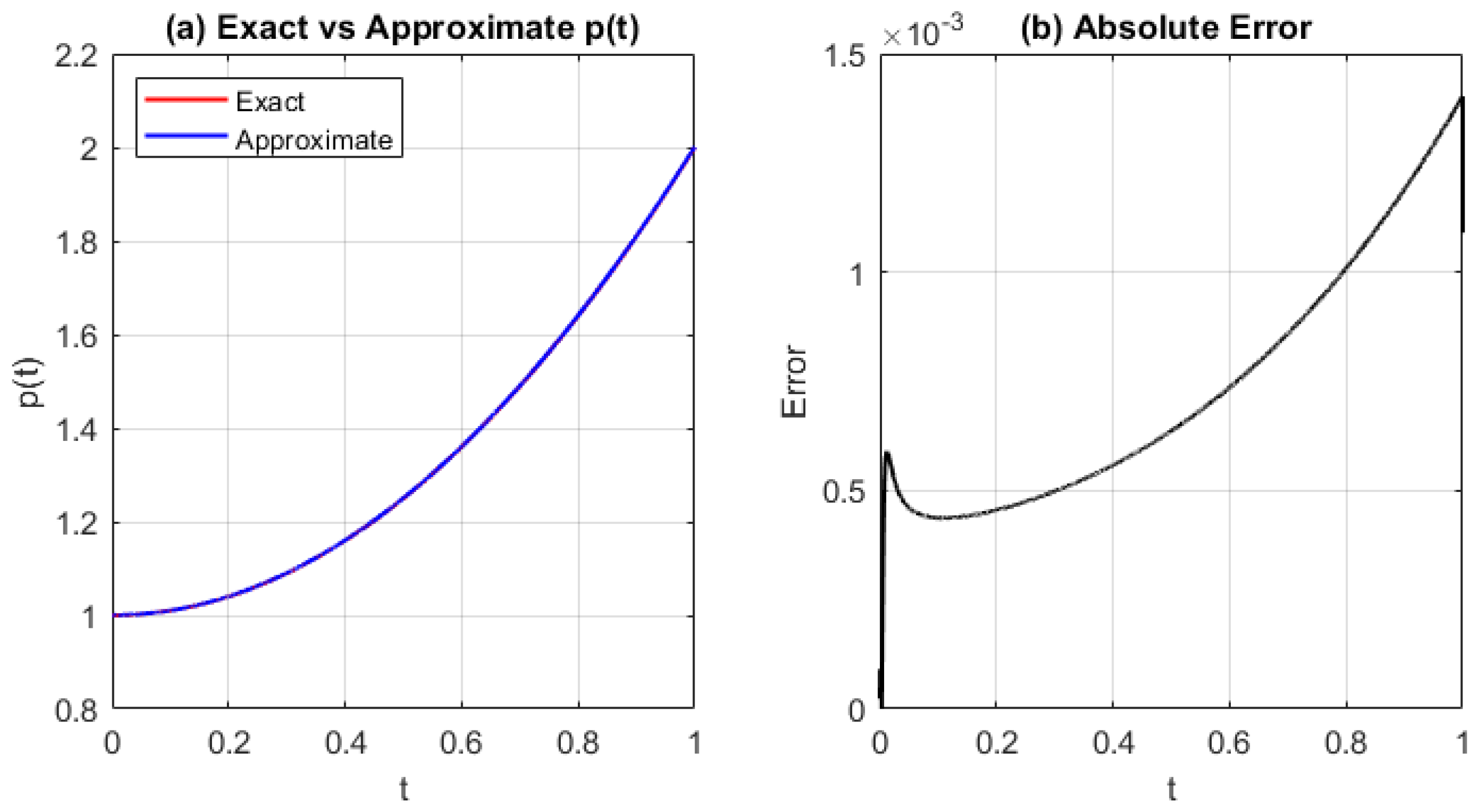
(a) Exact and approximated source function , and (b) absolute error for Test Problem 1 using the GRBF with step size and shape parameter . The error remains small throughout the interval, with a generally increasing trend.
Figure 5.
(a) Exact and approximated source function , and (b) absolute error for Test Problem 1 using the GRBF with step size and shape parameter . The error remains small throughout the interval, with a generally increasing trend.
Figure 6.
(
a) Comparison of the exact and approximated source function
and (
b) the absolute error
for Test Problem 1 using the MQRBF. Results are computed with step size
and shape parameter
. The MQRBF yields lower error than the GRBF (
Figure 3), with stable performance across the time interval.
Figure 6.
(
a) Comparison of the exact and approximated source function
and (
b) the absolute error
for Test Problem 1 using the MQRBF. Results are computed with step size
and shape parameter
. The MQRBF yields lower error than the GRBF (
Figure 3), with stable performance across the time interval.
Figure 7.
(a) Exact and approximated source function and (b) the absolute error using MQRBF for and shape parameter . The error decreases significantly compared to coarser grids, confirming improved resolution and accuracy with finer discretization.
Figure 7.
(a) Exact and approximated source function and (b) the absolute error using MQRBF for and shape parameter . The error decreases significantly compared to coarser grids, confirming improved resolution and accuracy with finer discretization.
Figure 8.
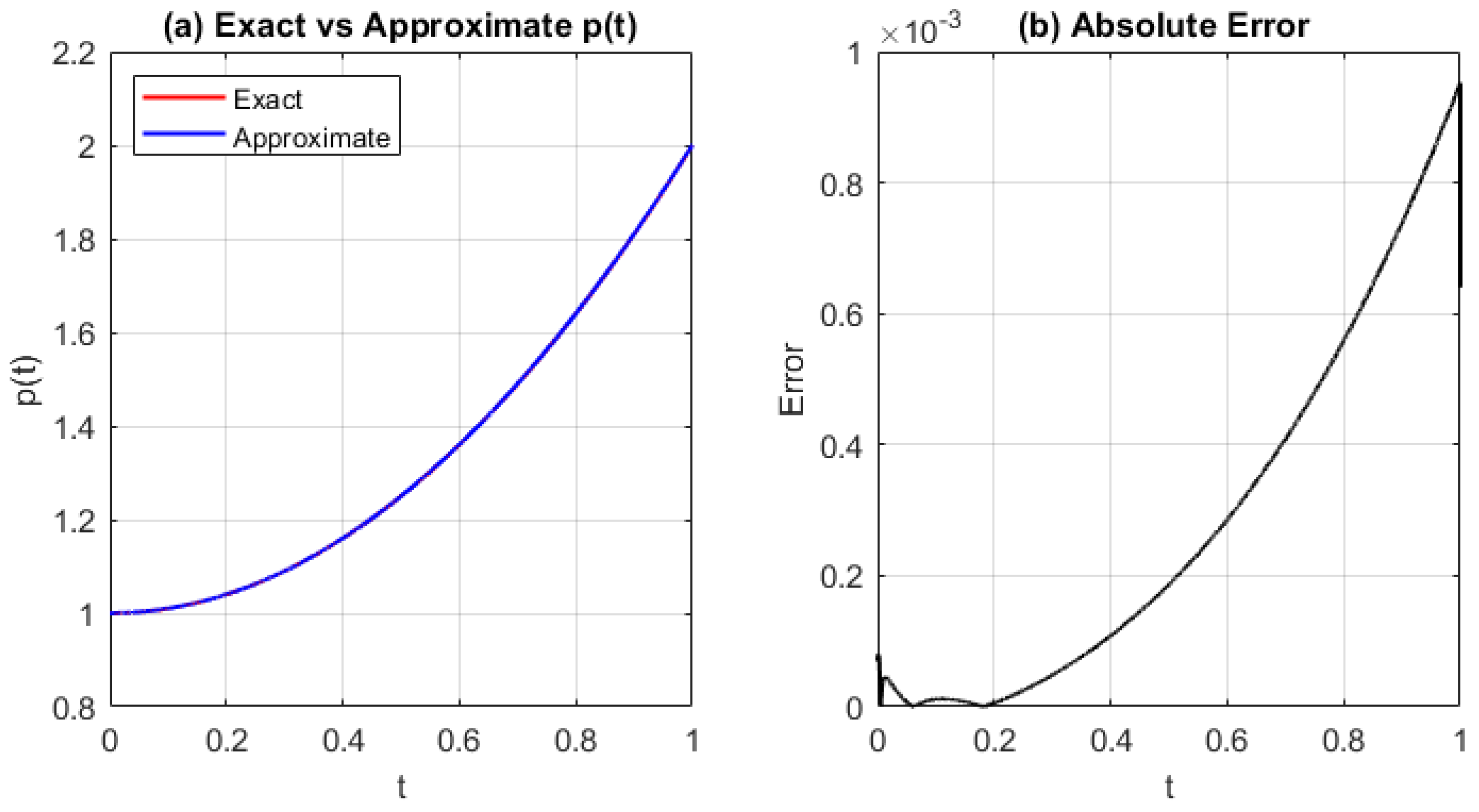
(a) Approximated source function and (b) the absolute error using the MQRBF with fine resolution and shape parameter . The results show excellent agreement with the exact solution and minimal error, indicating strong stability and convergence of the MQRBF at fine scales.
Figure 8.
(a) Approximated source function and (b) the absolute error using the MQRBF with fine resolution and shape parameter . The results show excellent agreement with the exact solution and minimal error, indicating strong stability and convergence of the MQRBF at fine scales.
Figure 9.
(a) Comparison of the exact and approximated source function and (b) the absolute error for Test Problem 1 using the IMQRBF with and shape parameter . The IMQRBF produces accurate results with reasonable error levels across the time interval.
Figure 9.
(a) Comparison of the exact and approximated source function and (b) the absolute error for Test Problem 1 using the IMQRBF with and shape parameter . The IMQRBF produces accurate results with reasonable error levels across the time interval.
Figure 10.
(a) Exact and approximated source function and (b) the absolute error using the IMQRBF with and . The results exhibit improved accuracy compared to coarser grids.
Figure 10.
(a) Exact and approximated source function and (b) the absolute error using the IMQRBF with and . The results exhibit improved accuracy compared to coarser grids.
Figure 11.
(a) Approximation of the source function and (b) absolute error using the IMQRBF for and . The numerical solution shows strong convergence toward the exact solution, with error remaining small.
Figure 11.
(a) Approximation of the source function and (b) absolute error using the IMQRBF for and . The numerical solution shows strong convergence toward the exact solution, with error remaining small.
Figure 12.
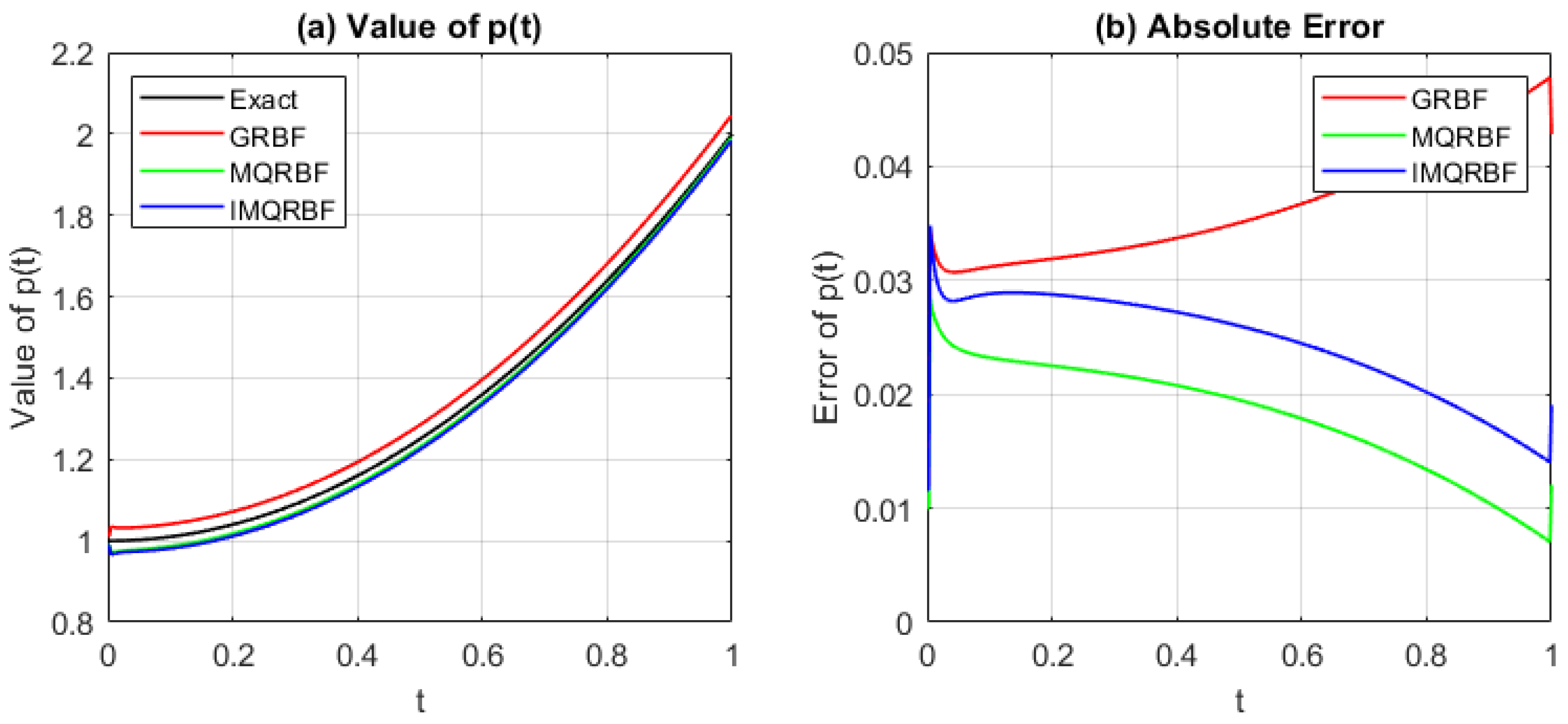
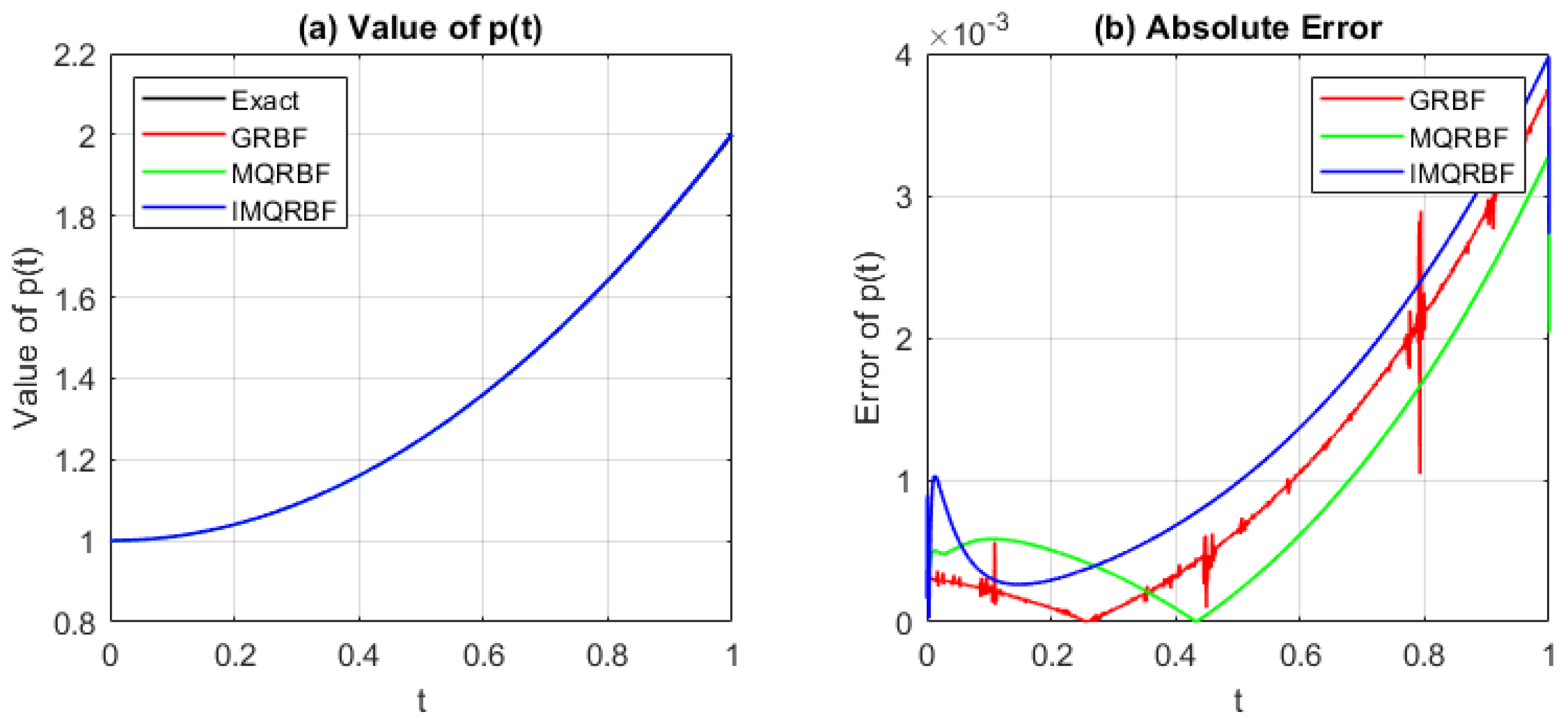
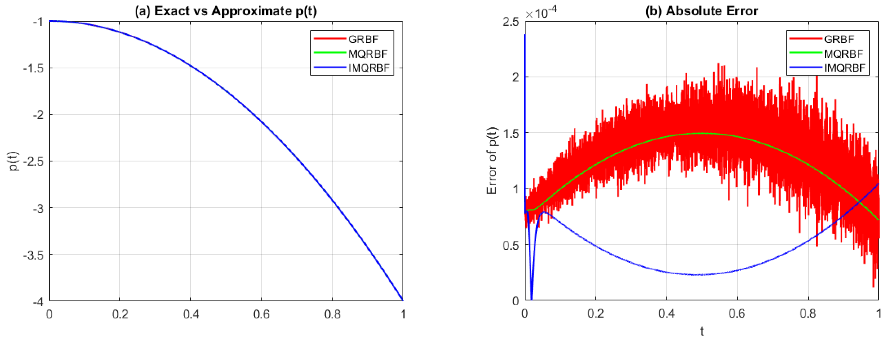
(a) Comparison of the approximated source function and (b) absolute error using GRBF, MQRBF, and IMQRBF with and . MQRBF yields the lowest error, demonstrating strong performance at coarse resolution.
Figure 12.
(a) Comparison of the approximated source function and (b) absolute error using GRBF, MQRBF, and IMQRBF with and . MQRBF yields the lowest error, demonstrating strong performance at coarse resolution.
Figure 13.
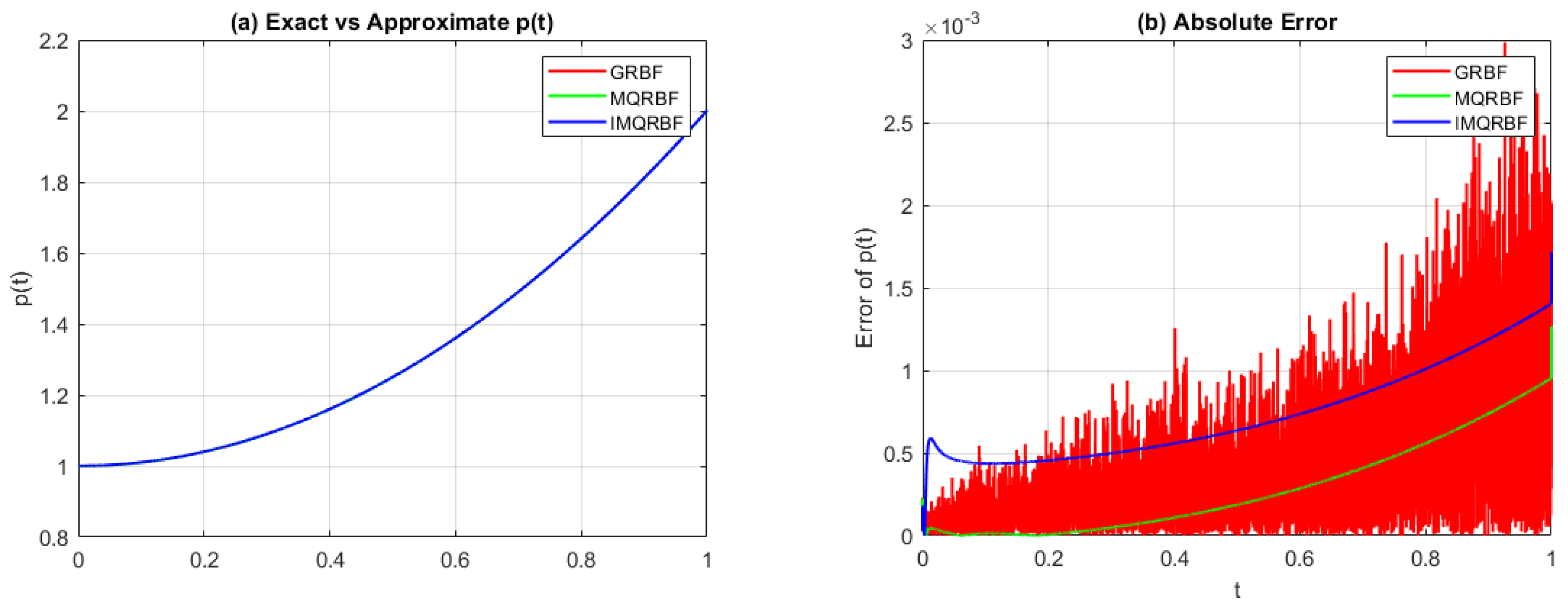
(a) Approximated source function and (b) absolute error for Test Problem 1 using three different RBFs with and . MQRBF outperforms others, providing the most stable and accurate results.
Figure 13.
(a) Approximated source function and (b) absolute error for Test Problem 1 using three different RBFs with and . MQRBF outperforms others, providing the most stable and accurate results.
Figure 14.
(a) Approximated source function and (b) absolute error with resolution . MQRBF consistently produces the smallest errors, confirming its effectiveness for high-resolution computations.
Figure 14.
(a) Approximated source function and (b) absolute error with resolution . MQRBF consistently produces the smallest errors, confirming its effectiveness for high-resolution computations.
Figure 15.
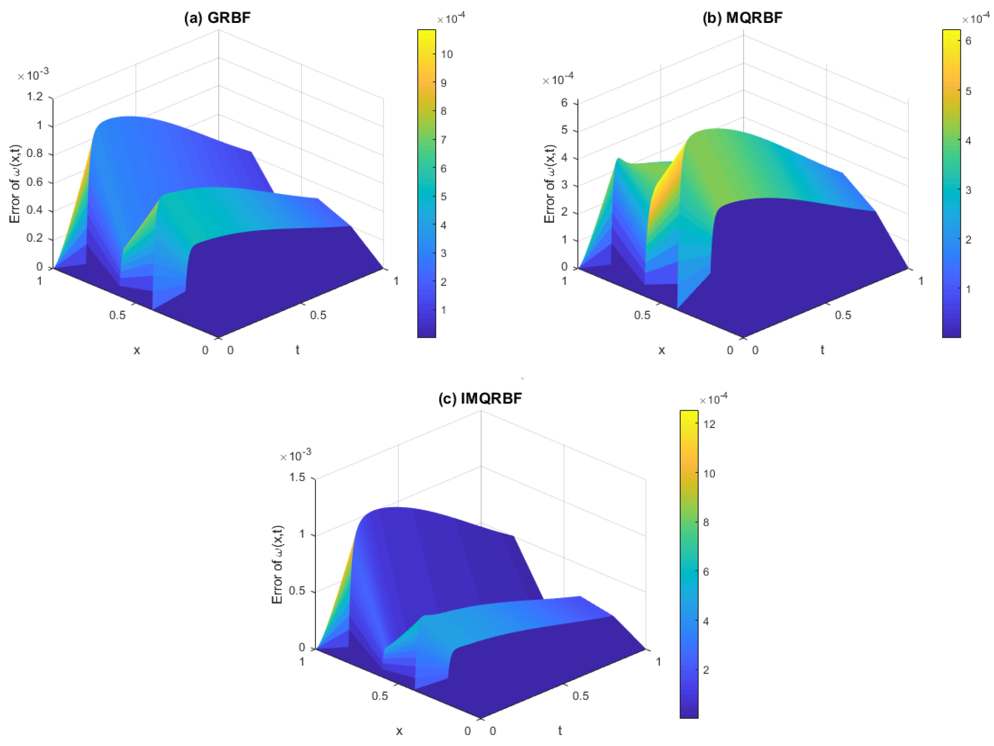
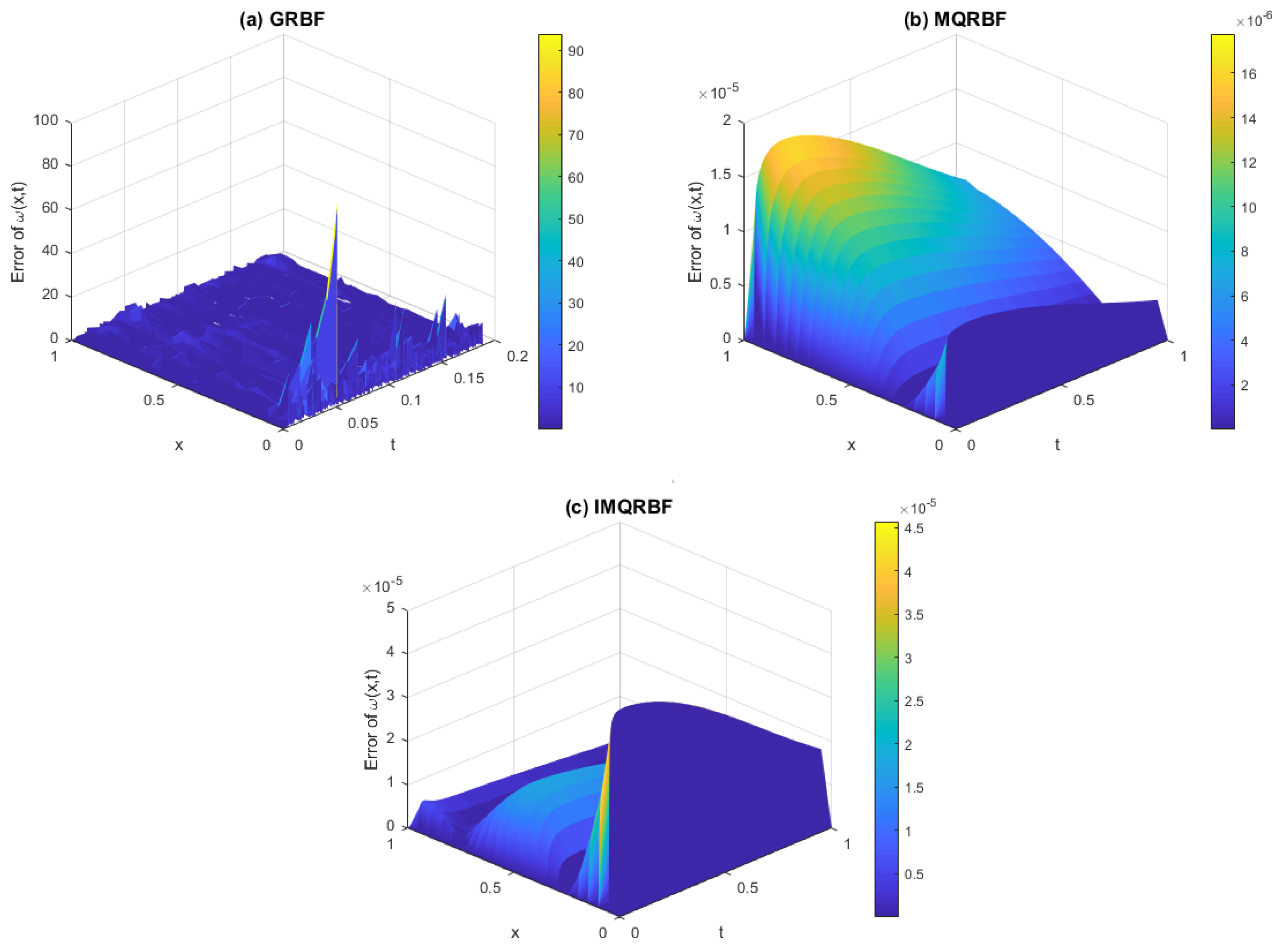
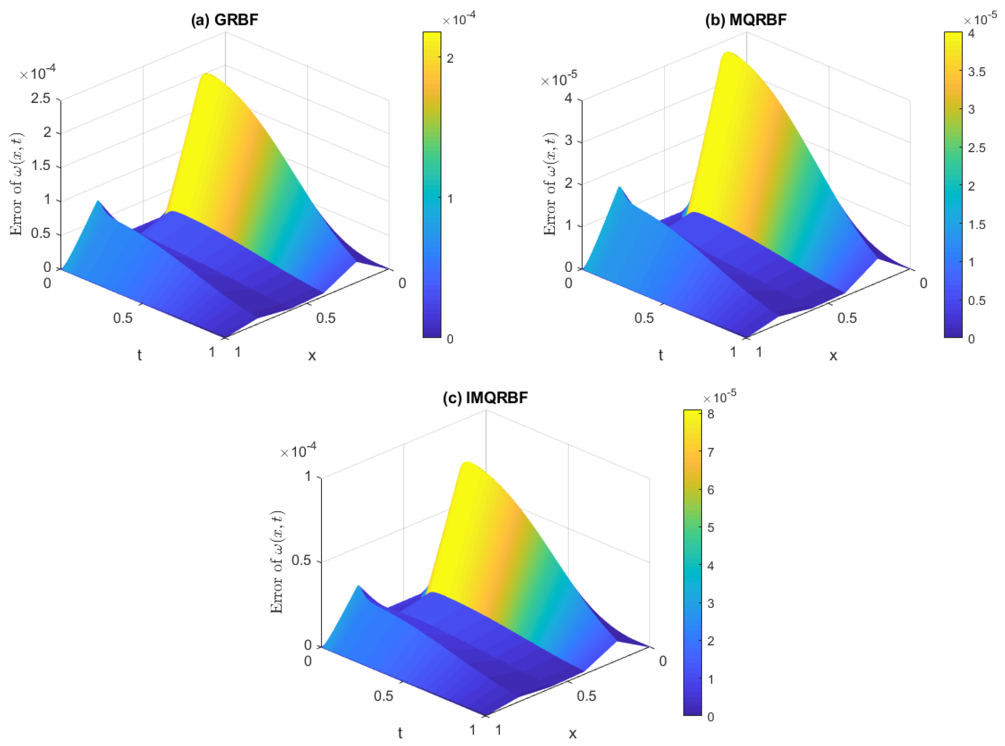
Approximation error using (a) GRBF, (b) MQRBF, and (c) IMQRBF for Test Problem 1 with spatial step size and shape parameter . Among the three, MQRBF yields the lowest error across the domain, showing its robustness at moderate resolution.
Figure 15.
Approximation error using (a) GRBF, (b) MQRBF, and (c) IMQRBF for Test Problem 1 with spatial step size and shape parameter . Among the three, MQRBF yields the lowest error across the domain, showing its robustness at moderate resolution.
Figure 16.
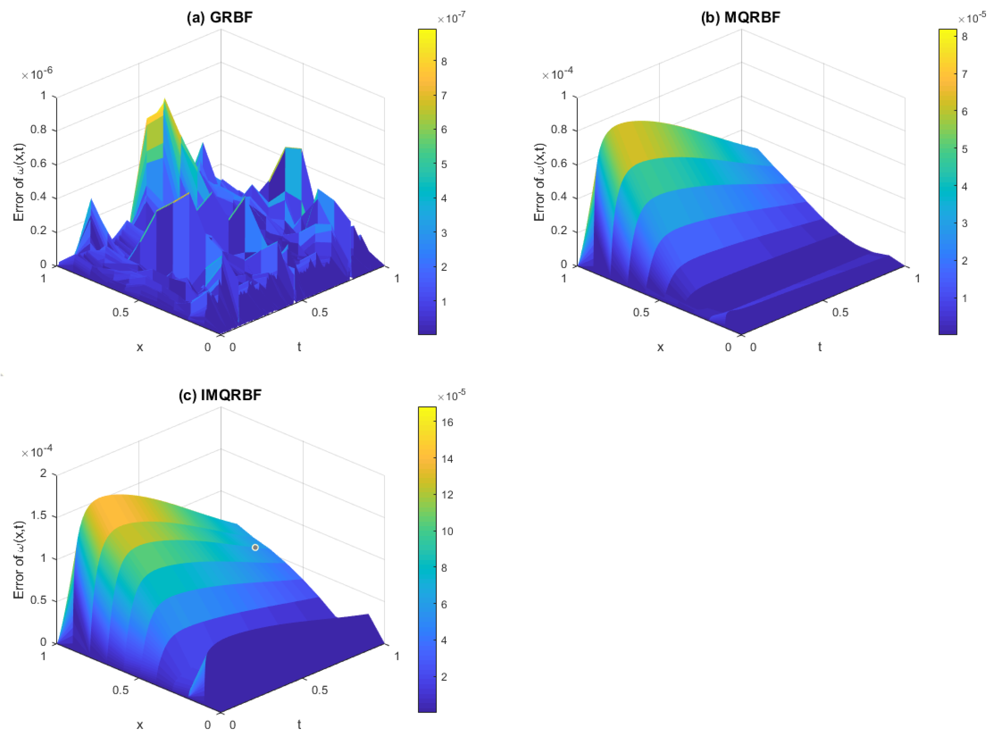
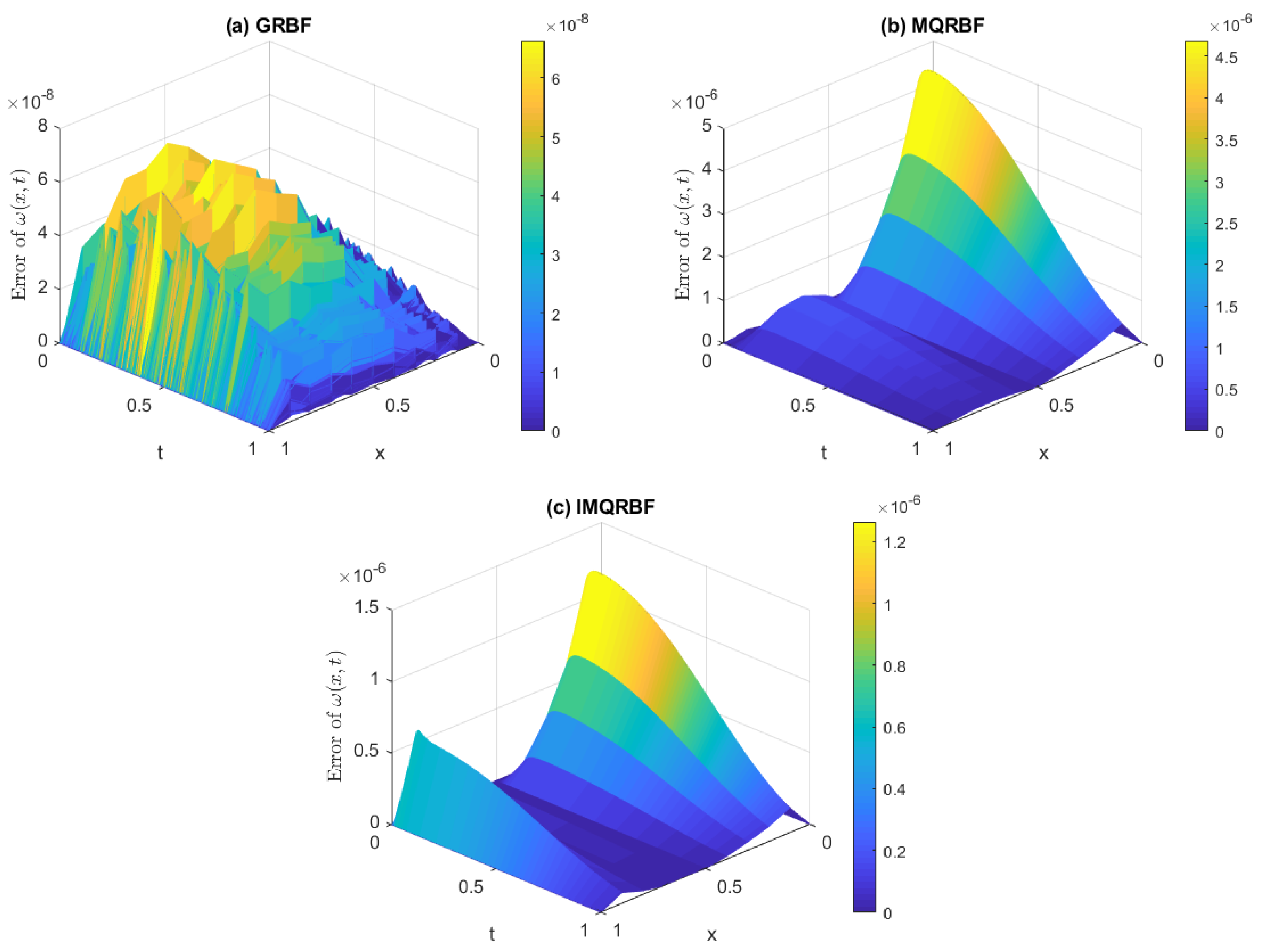
Approximation error for Test Problem 1 using (a) GRBF, (b) MQRBF, and (c) IMQRBF with spatial step size . The GRBF yields relatively small but fluctuating errors across the domain, while the MQRBF achieves smoother and more stable performance.
Figure 16.
Approximation error for Test Problem 1 using (a) GRBF, (b) MQRBF, and (c) IMQRBF with spatial step size . The GRBF yields relatively small but fluctuating errors across the domain, while the MQRBF achieves smoother and more stable performance.
Figure 17.
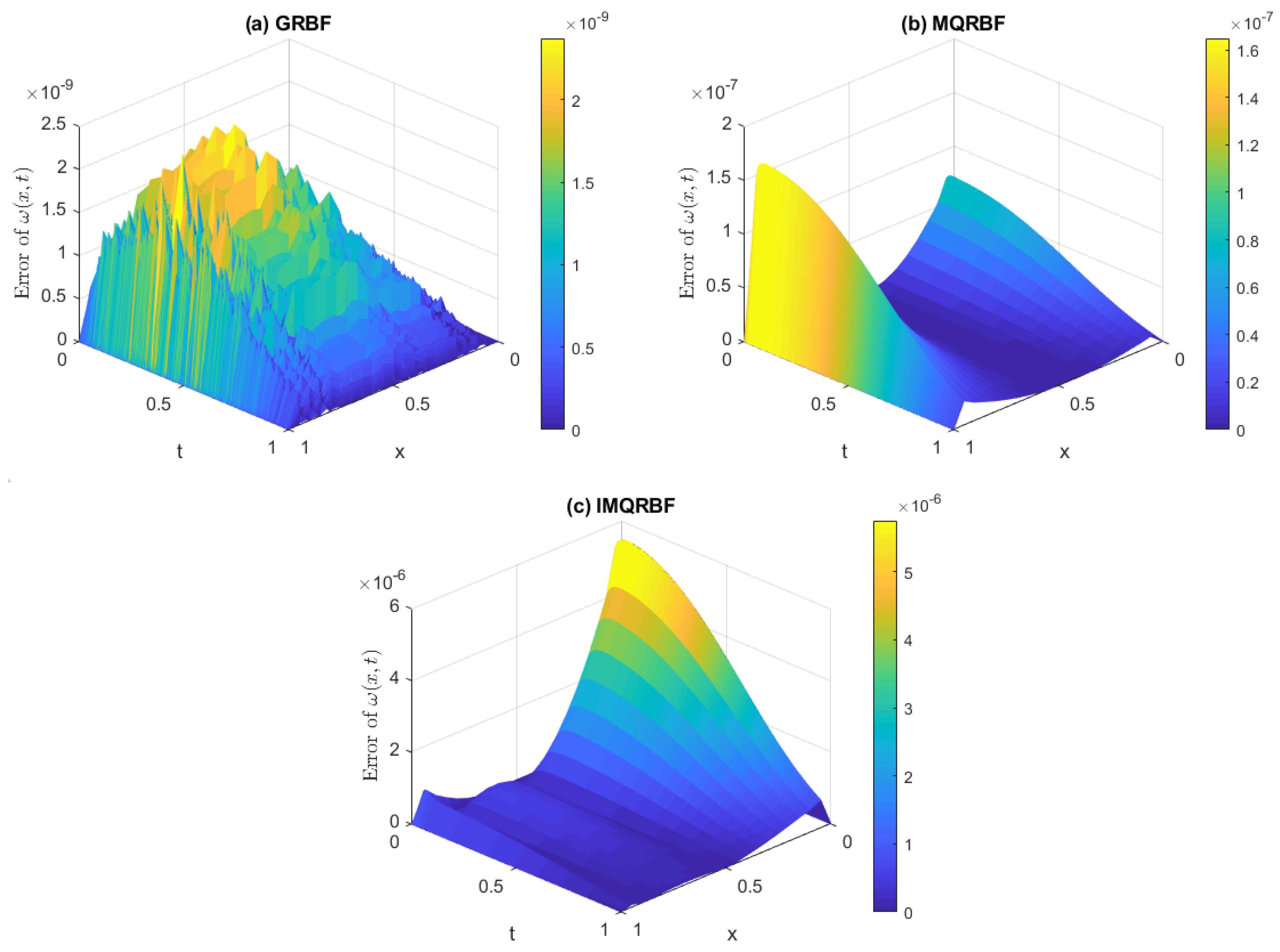
Absolute error computed using (a) GRBF, (b) MQRBF, and (c) IMQRBF for Test Problem 1 at high resolution () with shape parameter . MQRBF yields the most accurate and smoothest error profile, confirming its superior performance for finely discretized inverse parabolic problems.
Figure 17.
Absolute error computed using (a) GRBF, (b) MQRBF, and (c) IMQRBF for Test Problem 1 at high resolution () with shape parameter . MQRBF yields the most accurate and smoothest error profile, confirming its superior performance for finely discretized inverse parabolic problems.
Figure 18.
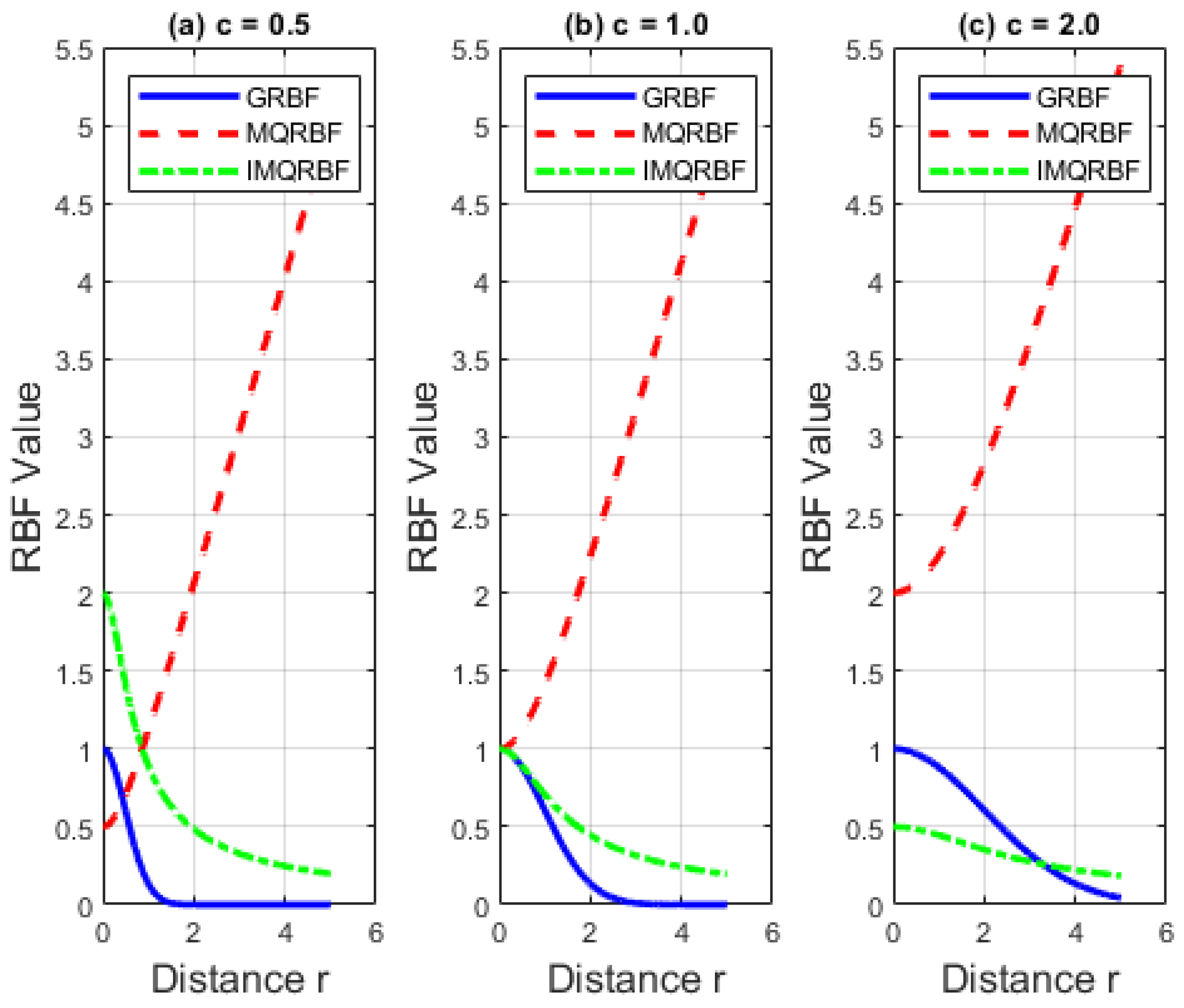
Comparison of GRBF, MQRBF, and IMQRBF radial basis functions for different shape parameters (a) , (b) , and (c) .
Figure 18.
Comparison of GRBF, MQRBF, and IMQRBF radial basis functions for different shape parameters (a) , (b) , and (c) .
Figure 19.
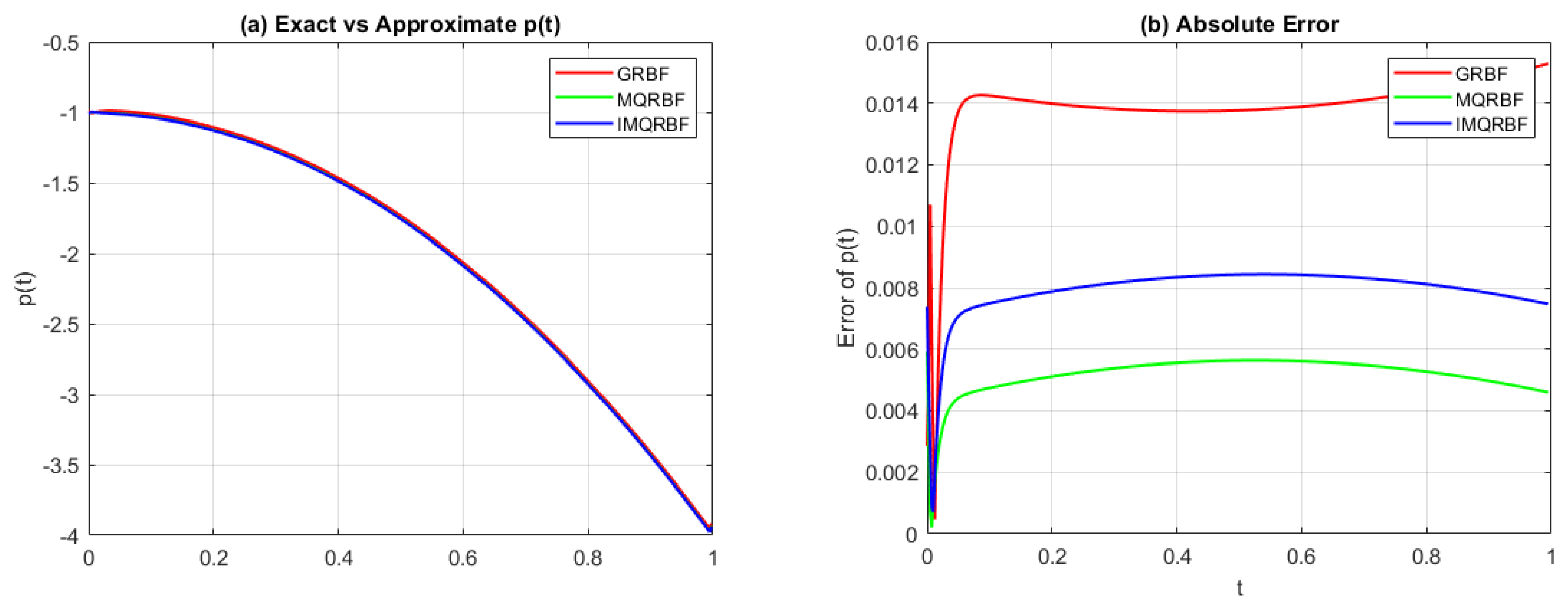
(a) Comparison of the approximated source function and (b) the absolute error for Test Problem 2 using GRBF, MQRBF and IMQRBF at coarse resolution with shape parameter . MQRBF performs better at this resolution.
Figure 19.
(a) Comparison of the approximated source function and (b) the absolute error for Test Problem 2 using GRBF, MQRBF and IMQRBF at coarse resolution with shape parameter . MQRBF performs better at this resolution.
Figure 20.
(a) Approximated source function and (b) absolute error for Test Problem 2 using the three RBFs at medium resolution . The IMQRBF shows the lowest overall error, demonstrating its increased accuracy and robustness at finer discretization levels.
Figure 20.
(a) Approximated source function and (b) absolute error for Test Problem 2 using the three RBFs at medium resolution . The IMQRBF shows the lowest overall error, demonstrating its increased accuracy and robustness at finer discretization levels.
Figure 21.
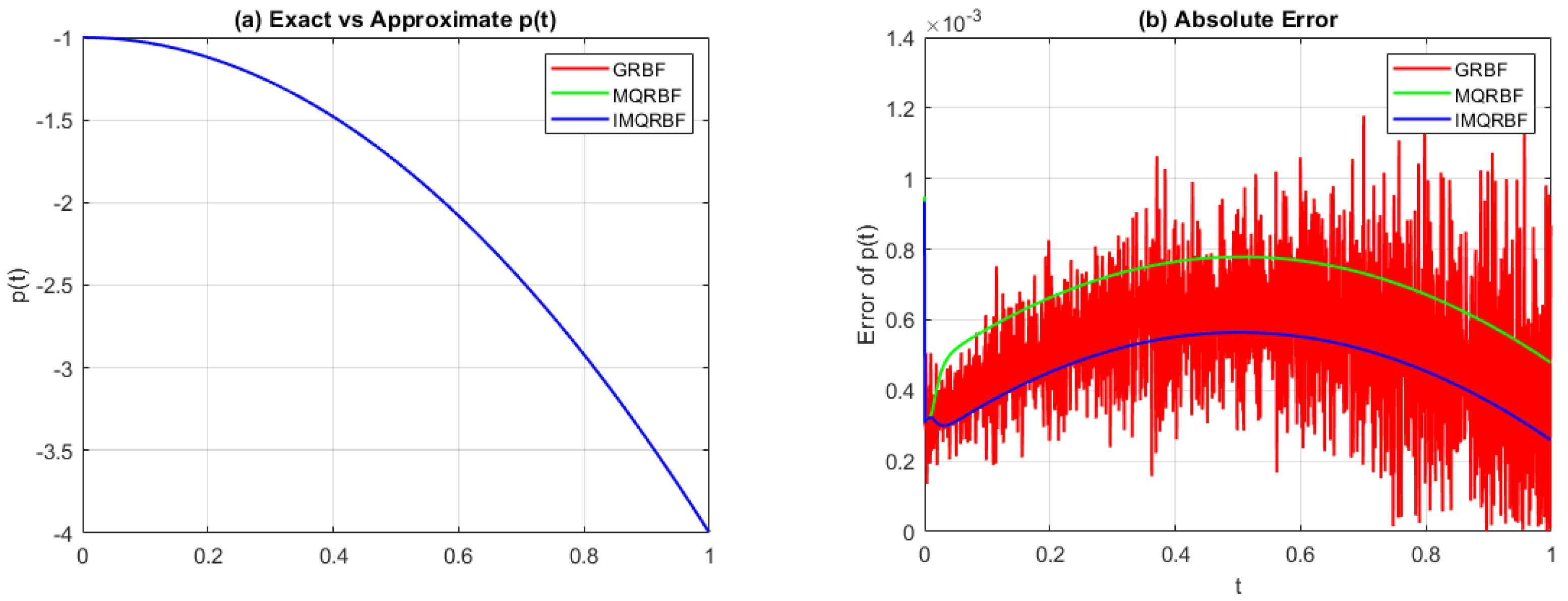
(a) Comparison of source control parameter approximation and (b) the absolute error for Test Problem 2 using GRBF, MQRBF, and IMQRBF with fine resolution . IMQRBF provides the most accurate and stable approximation, exhibiting significantly reduced error across the entire time domain.
Figure 21.
(a) Comparison of source control parameter approximation and (b) the absolute error for Test Problem 2 using GRBF, MQRBF, and IMQRBF with fine resolution . IMQRBF provides the most accurate and stable approximation, exhibiting significantly reduced error across the entire time domain.
Figure 22.
Absolute error for Test Problem 2 using (a) GRBF, (b) MQRBF, and (c) IMQRBF at coarse resolution and shape parameter . All three methods yield similar error magnitudes, with MQRBF slightly outperforming the others near the boundaries.
Figure 22.
Absolute error for Test Problem 2 using (a) GRBF, (b) MQRBF, and (c) IMQRBF at coarse resolution and shape parameter . All three methods yield similar error magnitudes, with MQRBF slightly outperforming the others near the boundaries.
Figure 23.
Error in the numerical solution for Test Problem 2 using (a) GRBF, (b) MQRBF, and (c) IMQRBF at . Although GRBF yields the lowest error magnitudes, its strong fluctuations reduce reliability. MQRBF and IMQRBF offer smoother, more stable errors, with IMQRBF showing the most consistent performance in the interior region.
Figure 24.
Error in the numerical solution for Test Problem 2 using (a) GRBF, (b) MQRBF, and (c) IMQRBF at . The results show similar behavior to the case: although GRBF yields the lowest error magnitudes, its strong fluctuations reduce reliability. MQRBF and IMQRBF provide smoother, more stable errors, with MQRBF maintaining the most consistent accuracy in the interior region.
Figure 25.
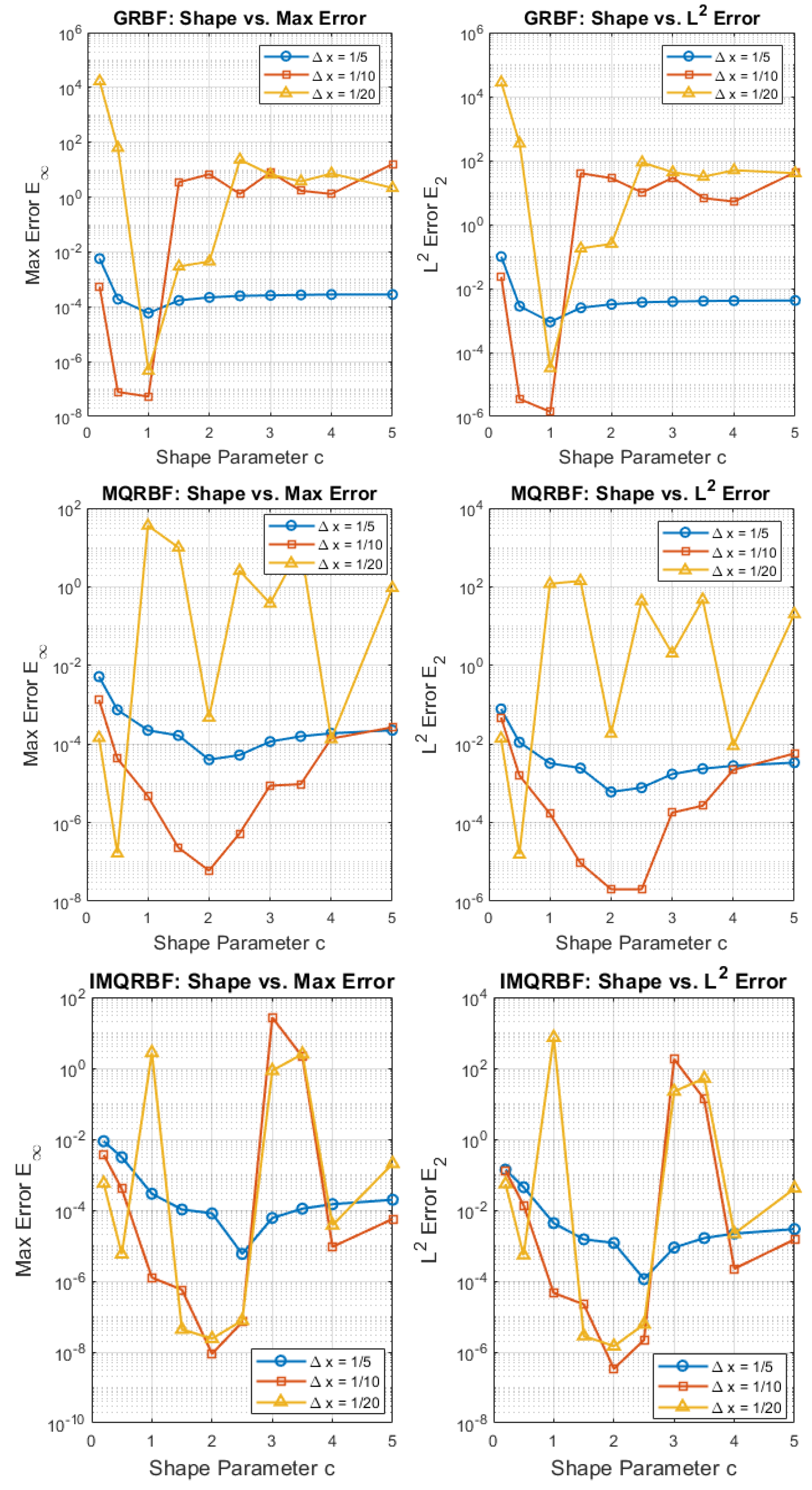
Comparison of shape parameter sensitivity for GRBF, MQRBF, and IMQRBF. Each panel shows the variation in the maximum error and error with shape parameter c for three spatial resolutions. GRBF performs best near , while both MQRBF and IMQRBF achieve optimal accuracy and stability around , with IMQRBF showing the most robust behavior across resolutions.
Figure 26.
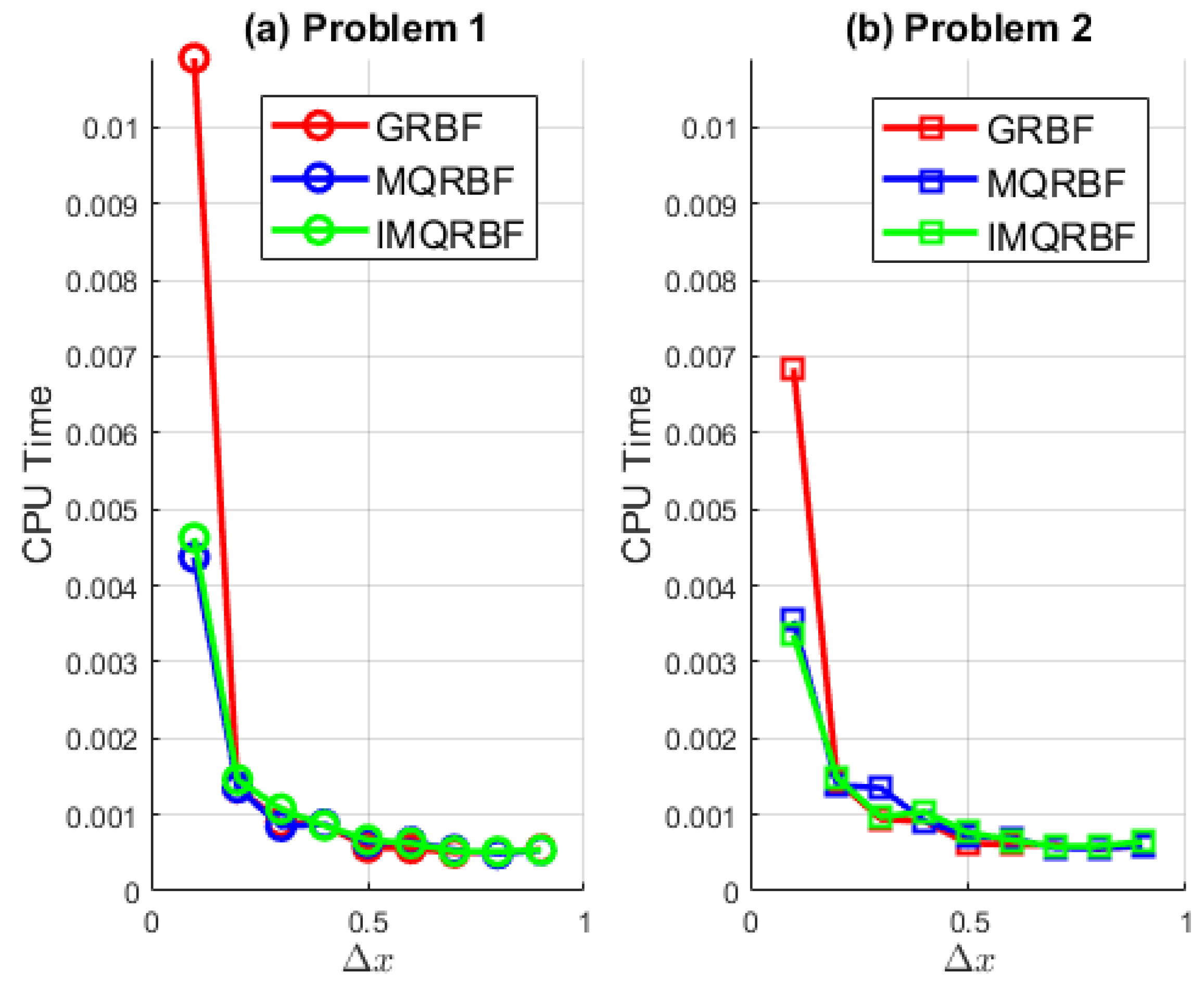
CPU time vs. for three RBF methods applied to (a) Problem 1 and (b) Problem 2.
Figure 26.
CPU time vs. for three RBF methods applied to (a) Problem 1 and (b) Problem 2.
Figure 27.
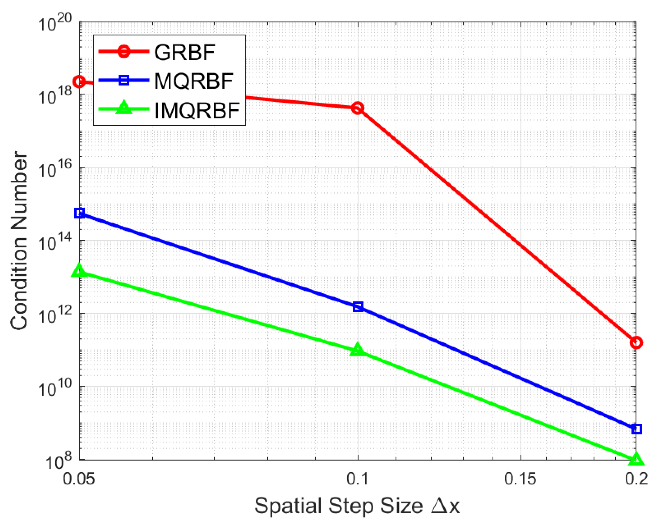
Log–log plot of the condition number of the collocation matrix versus the spatial step size for GRBF, MQRBF, and IMQRBF. As the resolution increases (i.e., decreases), the condition number grows significantly—most severely for the GRBF. The IMQRBF exhibits the slowest growth in ill-conditioning, indicating superior numerical stability.
Table 1.
Some common choices for RBFs.
Table 1.
Some common choices for RBFs.
| Function Name | Mathematical Definition |
|---|
| Cubic | |
| Gaussian (GRBF) | |
| Hardy Multiquadric (MQRBF) | |
| Inverse Multiquadric (IMQRBF) | |
| Inverse Quadratic (IQ) | |
| Thin plate spline | |
Table 2.
Description of subregions and applied conditions in the RBF collocation method.
Table 2.
Description of subregions and applied conditions in the RBF collocation method.
| Region | Condition Applied | Description |
|---|
| | Initial condition for all
x at |
| | Left boundary condition at , |
| | Right boundary condition at , |
| | Governing PDE applied in the interior domain |
| | Energy overspecification condition at internal point |
Table 3.
Maximum error norm and error norm for the approximation of using GRBF with shape parameter values and spatial step sizes . The lowest error for GRBF occurs near , but stability deteriorates for both smaller and larger c, especially at fine resolution. (The minimum error for each column is highlighted in bold).
| Shape Parameter | | | |
|---|
| Error
| Error
| Error | Error | Error | Error |
|---|
| | | | | | |
| | | | | | |
| | | | | | |
| | | | | | |
| | | | | | |
| | | | | | |
| | | | | | |
| | | | | | |
| | | | | | |
| | | | | | |
Table 4.
Maximum error norm and error norm for the approximation of using MQRBF with shape parameter values and spatial step sizes . For the MQRBF, the lowest errors occur near shape parameter , particularly for the medium resolution . The method shows good numerical performance over a broader range of c values compared to GRBF. (The minimum error for each column is highlighted in bold).
| Shape Parameter | | | |
|---|
| Error | Error | Error | Error | Error | Error |
|---|
| | | | | | |
| | | | | | |
| | | | | | |
| | | | | | |
| | | | | | |
| | | | | | |
| | | | | | |
| | | | | | |
| | | | | | |
| | | | | | |
Table 5.
Maximum error norm and error norm for the approximation of using IMQRBF for shape parameter values and spatial step sizes . The IMQRBF demonstrates strong numerical stability across all tested shape parameters and resolutions. Optimal performance is consistently achieved near . (The minimum error for each column is highlighted in bold).
| Shape Parameter | | | |
|---|
|
Error
|
Error
|
Error
|
Error
|
Error
|
Error
|
|---|
| | | | | | |
| | | | | | |
| | | | | | |
| | | | | | |
| | | | | | |
| | | | | | |
| | | | | | |
| | | | | | |
| | | | | | |
| | | | | | |
Table 6.
Maximum error norm and error norm using GRBF for Test problem 2. The lowest error for GRBF occurs near , but stability deteriorates for both smaller and larger c, especially at fine resolution. (The minimum error for each column is highlighted in bold).
Table 6.
Maximum error norm and error norm using GRBF for Test problem 2. The lowest error for GRBF occurs near , but stability deteriorates for both smaller and larger c, especially at fine resolution. (The minimum error for each column is highlighted in bold).
| Shape Parameter | Δx =
| Δx = | Δx = |
|---|
|
Error
|
Error
|
Error
|
Error
|
Error
|
Error
|
|---|
| | | | | | |
| | | | | | |
| | | | | | |
| | | | | | |
| | | | | | |
| | | | | | |
| | | | | | |
| | | | | | |
| | | | | | |
| | | | | | |
Table 7.
Maximum error norm and error norm using MQRBF for shape parameter values and . The lowest error for occurs near . (The minimum error for each column is highlighted in bold).
Table 7.
Maximum error norm and error norm using MQRBF for shape parameter values and . The lowest error for occurs near . (The minimum error for each column is highlighted in bold).
| Shape Parameter | Δx = | Δx = | Δx = |
|---|
|
Error
|
Error
|
Error
|
Error
|
Error
|
Error
|
|---|
| | | | | | |
| | | | | | |
| | | | | | |
| | | | | | |
| | | | | | |
| | | | | | |
| | | | | | |
| | | | | | |
| | | | | | |
| | | | | | |
Table 8.
Maximum error norm and error norm using IMQRBF for shape parameter values and . The lowest error for IMQRBF occurs near . (The minimum error for each column is highlighted in bold).
Table 8.
Maximum error norm and error norm using IMQRBF for shape parameter values and . The lowest error for IMQRBF occurs near . (The minimum error for each column is highlighted in bold).
| Shape Parameter | Δx = | Δx = | Δx = |
|---|
|
Error
|
Error
|
Error
|
Error
|
Error
|
Error
|
|---|
| | | | | | |
| | | | | | |
| | | | | | |
| | | | | | |
| | | | | | |
| | | | | | |
| | | | | | |
| | | | | | |
| | | | | | |
| | | | | | |
Table 9.
Measured CPU time (in seconds) for each RBF method, test problem, and spatial step size .
Table 9.
Measured CPU time (in seconds) for each RBF method, test problem, and spatial step size .
| RBF | Problem | Δx = 0.1
| 0.2 | 0.3 | 0.4 | 0.5 | 0.6 | 0.7 | 0.8 | 0.9 |
|---|
| GRBF | Problem 1 | 0.0123 | 0.0013 | 0.0009 | 0.0009 | 0.0007 | 0.0005 | 0.0005 | 0.0005 | 0.0005 |
| | Problem 2 | 0.0052 | 0.0013 | 0.0009 | 0.0012 | 0.0006 | 0.0006 | 0.0006 | 0.0006 | 0.0005 |
| MQRBF | Problem 1 | 0.0044 | 0.0014 | 0.0008 | 0.0009 | 0.0006 | 0.0007 | 0.0005 | 0.0005 | 0.0005 |
| | Problem 2 | 0.0034 | 0.0014 | 0.0009 | 0.0009 | 0.0007 | 0.0008 | 0.0006 | 0.0006 | 0.0006 |
| IMQRBF | Problem 1 | 0.0047 | 0.0014 | 0.0008 | 0.0008 | 0.0006 | 0.0006 | 0.0005 | 0.0005 | 0.0006 |
| | Problem 2 | 0.0032 | 0.0014 | 0.0009 | 0.0009 | 0.0007 | 0.0007 | 0.0007 | 0.0006 | 0.0006 |
Table 10.
Condition numbers of the collocation matrix for different RBFs at spatial step sizes . The final column shows the relative increase in condition number between and .
Table 10.
Condition numbers of the collocation matrix for different RBFs at spatial step sizes . The final column shows the relative increase in condition number between and .
| RBF | Δx = | Δx = | Δx = | Relative Increase |
|---|
| GRBF | | | | |
| MQRBF | | | | |
| IMQRBF | | | | |
Table 11.
Comparison of RBF types across different spatial resolutions for both test problems. Optimal shape parameters are based on lowest error.
Table 11.
Comparison of RBF types across different spatial resolutions for both test problems. Optimal shape parameters are based on lowest error.
| RBF Type | Optimal c | Best Resolution | Stability (Condition Number) | Performance Rank |
|---|
| GRBF | 1.0 | | Poor at fine grid | Moderate |
| MQRBF | 2.0 | | Moderate | Good |
| IMQRBF | 2.0 | | Excellent | Best |
