Abstract
Facial expression recognition (FER) is a critical research direction in artificial intelligence, which is widely used in intelligent interaction, medical diagnosis, security monitoring, and other domains. These applications highlight its considerable practical value and social significance. Face expression recognition models often need to run efficiently on mobile devices or edge devices, so the research on lightweight face expression recognition is particularly important. However, feature extraction and classification methods of lightweight convolutional neural network expression recognition algorithms mostly used at present are not specifically and fully optimized for the characteristics of facial expression images, yet fail to make full use of the feature information in face expression images. To address the lack of facial expression recognition models that are both lightweight and effectively optimized for expression-specific feature extraction, this study proposes a novel network design tailored to the characteristics of facial expressions. In this paper, we refer to the backbone architecture of MobileNet V2 network, and redesign LightExNet, a lightweight convolutional neural network based on the fusion of deep and shallow layers, attention mechanism, and joint loss function, according to the characteristics of the facial expression features. In the network architecture of LightExNet, firstly, deep and shallow features are fused in order to fully extract the shallow features in the original image, reduce the loss of information, alleviate the problem of gradient disappearance when the number of convolutional layers increases, and achieve the effect of multi-scale feature fusion. The MobileNet V2 architecture has also been streamlined to seamlessly integrate deep and shallow networks. Secondly, by combining the own characteristics of face expression features, a new channel and spatial attention mechanism is proposed to obtain the feature information of different expression regions as much as possible for encoding. Thus improve the accuracy of expression recognition effectively. Finally, the improved center loss function is superimposed to further improve the accuracy of face expression classification results, and corresponding measures are taken to significantly reduce the computational volume of the joint loss function. In this paper, LightExNet is tested on the three mainstream face expression datasets: Fer2013, CK+ and RAF-DB, respectively, and the experimental results show that LightExNet has 3.27 M Parameters and 298.27 M Flops, and the accuracy on the three datasets is 69.17%, 97.37%, and 85.97%, respectively. The comprehensive performance of LightExNet is better than the current mainstream lightweight expression recognition algorithms such as MobileNet V2, IE-DBN, Self-Cure Net, Improved MobileViT, MFN, Ada-CM, Parallel CNN(Convolutional Neural Network), etc. Experimental results confirm that LightExNet effectively improves recognition accuracy and computational efficiency while reducing energy consumption and enhancing deployment flexibility. These advantages underscore its strong potential for real-world applications in lightweight facial expression recognition.
1. Introduction
Facial expressions represent one of the most authentic and biologically significant channels for human emotional communication, providing direct insight into affective states. Facial expression recognition is a technology that analyzes and processes face images by computer to recognize the state of human facial expression [1]. In 1971, six basic facial expression categories were identified by famous psychologist Ekman [2]: Angry, Disgust, Fear, Happy, Sad, and Surprise. Neutral emojis have also been proposed as society continues to evolve, resulting in the current mainstream seven emoji states. Face Expression Recognition (FER) recognizes human facial expressions through several steps such as face detection, face alignment, feature extraction, and classification [3], and has been widely used in the fields of intelligent interaction, medical diagnosis, and security monitoring.
In terms of intelligent interaction, by recognizing the user’s facial expression, a more intelligent and natural interaction experience can be realized. In intelligent driving systems, facial expression recognition technology enables real-time monitoring of driver affective states, facilitating timely interventions to maintain alertness and thereby enhancing road safety. For instance, detection of fatigue or distraction patterns can trigger adaptive warning systems to prevent accidents. In addition, in the field of virtual reality and augmented reality, facial expression recognition technology can also realize a more immersive user experience, providing users with a richer and more vivid interactive experience [4]. In terms of medical diagnosis, by analyzing patients’ facial expressions, doctors can more accurately understand their emotional state and mental health status, thereby assisting in diagnosis and treatment [5]. Additionally, facial expression recognition technology can also be used for postoperative rehabilitation monitoring. During the postoperative rehabilitation process, the patient’s facial expressions can reflect their level of pain, comfort, and emotional state. By analyzing this information, doctors can adjust treatment plans in a timely manner and improve the effectiveness of rehabilitation therapy [6]. In the field of security and surveillance, face expression recognition technology has important application potentials [7]. By recognizing facial expressions in the surveillance area, the surveillance system can more accurately perceive the emotional state and behavioral intentions of the personnel, thus improving the intelligence and responsiveness of the surveillance system [8].
Currently, in the field of expression recognition research, the mainstream face expression recognition methods are mainly divided into traditional machine learning-based methods and deep learning-based methods. There are two main traditional machine learning methods for describing faces: geometric feature-based methods and texture feature-based methods. However, conventional machine learning methods often separate facial feature extraction from classification into distinct stages, resulting in complex operations and lack of joint optimization. The effectiveness of recognition depends on the discriminative power and robustness of manually designed features.
The meteoric rise of deep learning technology has injected new vitality into machine learning-based expression recognition methods. Unlike traditional methods, in deep learning methods both the process of feature extraction and classification can be done by the deep learning model itself. The stunning debut of AlexNet [9] in 2012 provided improvement ideas for neural network development, allowing numerous network models such as VGG-Nets [10], GoogleNet [11], ResNet [12], and DenseNet [13] to employ deepening of the network and enhancement of convolutional functionality to improve network recognition accuracy. The study in [14] proposed an identity-aware convolutional neural network using two convolutional neural networks for training, one for training features related to facial expressions and the other for training features related to identity, which improved the accuracy of expression recognition for different faces. Mollahosseini et al. [15] increased the width and depth of the network based on the Inception layer and achieved good results on datasets such as CK+. Study [16] proposed a fused convolutional neural network to improve the accuracy and robustness of facial expression recognition by extracting facial features through improved LeNet and ResNet, respectively, and then connecting the two feature vectors for classification. Lee et al. [17] designed a dual-stream coding network that extracts features from face and background regions, respectively, and combines them with scenarios for expression recognition so that reduces the ambiguity of network and improves the accuracy of emotion recognition. Study [18] proposed a self-cure network (SCN) that mitigates the problem of inaccurate labeling of large-scale facial expression datasets by weighting each sample in training through ranked regularization. Zhang et al. [19] proposed an Identity-Expression Dual Branch Network (IE-DBN) that can force the network to generate expression-guided identity-related features while suppressing negative identity factors and outperforms most current techniques. Sidhom et al. [20] proposed a novel three-phase hybrid feature selection method that leverages the strengths of filter, wrapper, and embedded algorithms. Mukhopadhyay et al. [21] presents a new facial expressions detection method by exploiting textural image features such as local binary patterns (LBP), local ternary patterns (LTP) and completed local binary pattern (CLBP). Fan et al. [22] first propose a deeply-supervised attention network (DSAN) to recognize human emotions based on facial images automatically. Based on DSAN, a two-stage training scheme is designed, taking full advantage of the race/gender/age-related information. Li et al. [23] adopt an Adaptive Confidence Margin (Ada-CM) to fully leverage all unlabeled data for semi-supervised deep facial expression recognition. All unlabeled samples are partitioned into two subsets by comparing their confidence scores with the adaptively learned confidence margin at each training epoch: (1) subset I including samples whose confidence scores are no lower than the margin; (2) subset II including samples whose confidence scores are lower than the margin. For samples in subset I, the predictions are constrained to match pseudo labels. Meanwhile, samples in subset II participate in the feature-level contrastive objective to learn effective facial expression features. Ada-CM is evaluated extensively on four challenging datasets, showing that the method achieves state-of-the-art performance, especially surpassing fully supervised baselines in a semi-supervised manner. The study of ablation further proves the effectiveness of the method.
With the continuous development and application of deep neural network models, the key indicators of network continue to improve, such as the depth, the width, the parameters number, the computation amount and so on. As neural networks become increasingly complex, deploying them on mobile and embedded devices becomes challenging. However, with the increasing demand for real-time, on-device facial expression recognition in mobile and embedded environments, there is an urgent need to develop lightweight FER models that offer competitive accuracy with significantly lower computational cost.
The necessity for lightweight FER models is driven by the rapid proliferation of edge computing and ubiquitous devices such as smartphones, smartwatches, AR/VR headsets, and in-vehicle monitoring systems. In such settings, computational resources, power availability, and memory capacity are often constrained. Heavy models are not suitable for these platforms due to their inference latency and energy consumption. In contrast, lightweight models can perform real-time inference directly on edge devices, reducing latency, enhancing user privacy by avoiding cloud transmission, and lowering bandwidth requirements.
Moreover, many practical FER applications, such as driver drowsiness detection, classroom engagement monitoring, and mobile mental health assessment, require continuous, long-term operation. Lightweight models consume significantly less power, making them ideal for battery-powered or energy-sensitive scenarios. They also facilitate large-scale deployment in scenarios such as intelligent surveillance or retail analytics, where hundreds of devices may need to operate simultaneously with minimal hardware cost.
Lightweight FER models also contribute positively to model generalizability and ethical deployment. By design, these models often have fewer parameters and simpler architectures, which may help mitigate overfitting, especially in scenarios with limited or imbalanced training data. Furthermore, performing emotion recognition locally on-device alleviates privacy concerns, aligning with data protection regulations such as GDPR and addressing growing public scrutiny of biometric technologies.
In summary, designing lightweight FER models is essential for bridging the gap between academic research and real-world applications. These models provide a feasible and scalable solution for deploying emotion recognition in practical, resource-constrained environments without sacrificing performance, making them a cornerstone of future FER systems.
Therefore, numerous researchers have begun to design new lightweight convolutional neural networks. The SqueezeNet proposed by Iandola [24] pioneered the development of lightweight convolutional neural networks. This model is composed of several FireModels combined with convolutional layers, fully connected layers, etc. The FireModel includes two parts, squeeze and expand, which reduce the number of parameters by first reducing and then increasing the dimensionality of the feature map. In 2017, Google proposed the MobileNet [25] model, which uses a depthwise separable convolution to replace traditional convolution operations. Depthwise separable convolution decomposes the traditional convolution layer into two steps, namely, deep convolution first and then point wise convolution. Because MobileNet uses a large number of 3 × 3 convolution kernels, using depthwise separable convolution instead of traditional convolution operations can reduce the computational load by about nine times. At the same time, MobileNet also provides a hyperparameter to control the width of the network, balancing the relationship between model accuracy and model size. Following this, Google proposed the Xception [26] model, which is based on the idea of the Inception model and uses depthwise separable convolutions to replace the Inception module, and introduces residual structures. In 2018, the Google team proposed the MobileNetV2 [27] model. Compared to the MobileNet model, MobileNetV2 introduces an inverted residual structure, which ascends and then descends the dimensions to enhance the propagation of gradients, and removes the ReLU activation function for the second pointwise convolution in the inverted residual module, preserving the diversity of features. ShuffleNet [28], proposed by Kuangxiang Technology, uses point grouping convolution instead of point convolution operation to reduce the amount of computation, and at the same time proposes a channel shuffle method to solve the problem of not being able to exchange information between different groups due to the use of grouping convolution. The ShuffleNetV2 [29] model proposed by Ma et al. in 2018 improves ShuffleNet and proposes four principles for designing lightweight networks: the same channel width minimizes the memory access cost (MAC), too many group convolutions increase the memory access cost (MAC), fragmentation operations within the network reduce parallelism, and element-by-element operations increase the memory consumption. According to these four principles, ShuffleNetV2 introduces channel split operation, replaces group convolution in ShuffleNet with point convolution, and postdates the channel mixing operation. In 2020, Han et al. [30] proposed the GhostNet model, in which they found that the feature maps generated by convolutional neural networks usually contain rich or even redundant feature maps, and thus these redundant feature maps can be generated directly using constant mapping, so that a large number of feature maps can be obtained with a small amount of computation. In 2019, Mingxing Tan et al. [31] proposed the EfficientNet model, where they used the Neural Architecture Search (NAS) technique to simultaneously explore the effects of input resolution, network depth, and network width on accuracy. There are also many scholars who, based on these lightweight models, have proposed improved algorithms with considerable effects for some specific application scenarios. For example, Zhu et al. [32] propose an improved strategy for the MobileNetV2 neural network(I-MobileNetV2) in response to problems such as large parameter quantities in existing deep convolutional neural networks and the shortcomings of the lightweight neural network MobileNetV2 such as easy loss of feature information, poor real-time performance, and low accuracy rate in facial emotion recognition tasks. To avoid the overfitting problem of the network model and improve the facial expression recognition effect of partially occluded facial images. Jiang et al. [33] propose an improved facial expression recognition algorithm based on MobileViT. Firstly, in order to obtain features that are useful and richer for experiments, deep convolution operations are added to the inverted residual blocks of this network, thus improving the facial expression recognition rate. Then, in the process of dimension reduction, the activation function can significantly improve the convergence speed of the model, and then quickly reduce the loss error in the training process, as well as to preserve the effective facial expression features as much as possible and reduce the overfitting problem. In study [34] as it is difficult to highlight the features of facial expressions in the study of global faces, due to the unique subtleties and complexity of facial expressions. To improve the robustness of expression recognition in natural environments and optimize model parameters, a lightweight facial expression recognition method based on multiregion fusion is proposed, which integrates local details and global features to realize a combination of coarse and fine granularity, thus improving the model’s efficacy in discriminating subtle changes in expressions. Study [35] presents an expression recognition method based on parallel CNN. Firstly, a series of preprocessing operations is performed on facial expression images. Then, a CNN with two parallel convolution and pooling structures, which can extract subtle expressions, is designed for facial expression images. This parallel structure has three different channels, in which each channel extract different image features and fuse the extracted features, finally, the previously merged features are sent to the Soft Max layer for expression classification. Wang et al. [36] randomly clipped face faces based on face key points and fed the clipping results into the network, which had many duplicate clipping regions although local details were considered. Mao et al. [37] propose POSTER++. It improves POSTER in three directions: cross-fusion, two stream, and multi-scale feature extraction. POSTER++ reached 92.21% on RAF-DB, 67.49% on AffectNet (7 cls) and 63.77% on AffectNet (8 cls), respectively, using only 8.4 G floating point operations (FLOPs) and 43.7 M parameters (Param). Zhang et al. [38] propose CF-DAN which comprises three parts:(1) a cross-fusion grouped dual-attention mechanism to refine local features and obtain global information; (2) a proposed C2 activation function construction method, which is a piecewise cubic polynomial with three degrees of freedom, requiring less computation with improved flexibility and recognition abilities, which can better address slow running speeds and neuron inactivation problems; and (3) a closed-loop operation between the self-attention distillation process and residual connections to suppress redundant information and improve the generalization ability of the model. The recognition accuracies on the RAF-DB, FERPlus, and AffectNet datasets were 92.78%, 92.02%, and 63.58%, respectively.
Despite these advancements, a significant knowledge gap remains: most existing lightweight FER models are designed by adapting general-purpose lightweight backbones, without specifically optimizing for the unique structural and semantic characteristics of facial expression images. As a result, these models often fail to fully utilize local expression cues—especially from key facial regions such as the eyes, mouth, and eyebrows—which are critical for emotion discrimination. In addition, many approaches either focus solely on architectural compression or rely heavily on post-processing modules, with limited integration of spatial–semantic guidance into the feature extraction process itself.
To address these limitations, we propose LightExNet, a novel lightweight CNN tailored specifically for facial expression recognition. The design of LightExNet builds upon the MobileNetV2 backbone, as MobileNet V2 offers both high accuracy and a small number of parameters, making it well suited for lightweight facial expression recognition. But introduces three key innovations to enhance expression-specific feature extraction and classification under constrained computational budgets:
- Shallow–Deep Feature Fusion: By integrating low-level shallow features with high-level deep representations, the network retains fine-grained local details while gaining semantic abstraction, thus improving multiscale perception and alleviating gradient vanishing in deeper layers.
- Improved Channel and Spatial Attention Mechanism: A task-specific attention module is introduced to assign higher weights to emotionally salient regions, enhancing the model’s ability to focus on expression-relevant facial components.
- Joint Loss Function with Center Loss Optimization: An improved center loss is employed to enhance intra-class compactness and inter-class separability, thereby improving classification performance without increasing model complexity.
The proposed LightExNet is evaluated on three benchmark datasets: FER2013, CK+, and RAF-DB. Experimental results show that LightExNet achieves competitive accuracy (69.17%, 97.37%, and 85.97%, respectively) with only 3.27 M parameters and 298.27 M FLOPs, outperforming several existing mainstream lightweight FER models in both accuracy and computational efficiency.
In summary, this work bridges the gap between lightweight model design and expression-specific feature optimization, contributing a practical solution for real-time FER deployment on resource-limited devices.
2. Materials and Methods
2.1. Introduction to MobileNet V2
MobileNet V2 is a lightweight convolutional neural network improved by the Google team in 2018 based on MobileNet V1. It has efficient architecture that balances high accuracy with low computational cost, which is essential for deployment on embedded and mobile devices with limited resources. Its use of depthwise separable convolutions significantly reduces model parameters and computation, enabling faster inference and smaller model size without sacrificing performance. The inverted residual blocks with linear bottlenecks enhance feature extraction by preserving important information and capturing fine-grained facial details necessary for accurate expression recognition. Furthermore, MobileNet V2 has widely available pretrained weights, facilitating transfer learning and improving generalization on facial expression datasets. Compared to V1, V2 has about 20% fewer trainable parameters and performs better in the 1000 classification of the ImageNet competition with higher accuracy. Compared to MobileNet V3 proposed by Google team in 2019, although MobileNet V3 is slightly better in terms of accuracy, the parameters of the model are about 1.5 times of MobileNet V2. As the sample of the facial expression dataset is small, and too many parameters of the model are easy to cause overfitting, so the algorithm chooses MobileNet V2, which combines both accuracy and small parameters, as the main network to improve. The recognition rate and parameter count (P/M) comparison of MobileNet series network in ImageNet competition 1000 classification are shown in the Table 1.

Table 1.
Comparison of different MobileNet Performance.
In Table 1, “224” indicates that the input image size is 224 × 224, “recognition rate/%” is the top1 accuracy rate, and “P/M” is the parametric size of the model.
The main features of MobileNet V2 include: the use of 3 × 3 depth separable convolution instead of conventional convolution, which can significantly reduce the number of trainable parameters and speed up the training speed of the model. The use of the inverted residual structure first expands the input feature map and then reduces its dimensionality, allowing residual connections after feature extraction. This increases the overall network depth, enabling the model to capture higher-dimensional features and enhancing its feature representation capability. In addition, replacing the ReLU activation function used in V1 with a linear activation function helps reduce the loss of low-dimensional features.
2.1.1. Deeply Separable Convolution
Depthwise Separable Convolution (DSC) is composed of a Depthwise Convolution followed by a Pointwise Convolution. Unlike conventional convolution (shown in Figure 1), depthwise convolution does the convolution operation on only one channel of the input image for each convolution kernel during the convolution operation, and the number of convolution kernels is equal to the number of channels of the input image. Point-by-point convolution is a special case of regular convolution, i.e., ordinary convolution with a convolution kernel size of 1 × 1. Pointwise convolution does not alter the spatial dimensions of the feature map, it only changes the number of channels. The schematic diagram of depth separable convolution, is shown in Figure 2. The channels of the input feature map are first convolved using depth convolution to obtain the corresponding channel features, and then the extracted channel features are associated using point-by-point convolution. In the Figure 1 and Figure 2, and M are the edge length and the number of channels of the input feature graph, is the edge length of the deep convolution kernel, and N is the number of channels of ordinary convolution kernels or point-by-point convolution.
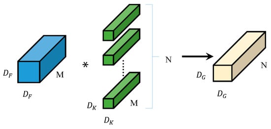
Figure 1.
Principle of Standard Convolution. In the figure, the blue blocks represent the input feature maps, while the green blocks indicate the convolution kernels applied to the input. The light yellow blocks denote the resulting output feature maps after the convolution operation. The asterisks (*) illustrate the specific positions where the input feature map and the convolution kernel are engaged in element-wise multiplication and summation during the convolution process.
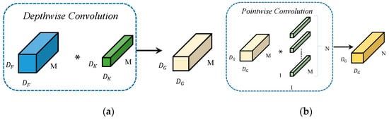
Figure 2.
(a) Principle of Depthwise Convolution (b) Principle of Pointwise Convolution. In the figure (a), the blue blocks represent the input feature maps, while the green blocks indicate the convolution kernels applied to the input. The light yellow blocks denote the resulting output feature maps after the convolution operation. The asterisks (*) illustrate depthwise convolution which does the convolution operation on only one channel of the in-put image for each convolution kernel during the convolution operation, and the number of convolution kernels is equal to the number of channels of the input image. In the figure (b), the light yellow blocks represent the input feature maps, and the green blocks denote the 1 × 1 convolution kernels applied to the input. The dark yellow blocks correspond to the resulting output feature maps generated by the convolution operation. The asterisks (*) indicate the positions where the input feature maps and the 1 × 1 convolution kernels perform element-wise multiplication and summation to produce the output.
Using DSC instead of ordinary convolution achieves the same effect and obtains the same feeling field, but with a large reduction in parameters and computation. Its parametric quantity comparison with ordinary convolution is shown in Equation (1).
In the Equation (1), and denote the number of parameters of depth-separable convolution and ordinary convolution under the same specification of convolution kernel, respectively. In the process of expression feature extraction, the MobileNet v2 model is usually composed of a stack of 3 × 3 convolutional kernels. As a result, the number of parameters in depthwise separable convolutions is approximately one-ninth that of standard convolutions.
2.1.2. Inverse Residual Structures with Linear Bottlenecks
Inspired by ResNet’s residual connection, MobileNet V2 adopts a reverse residual structure, aiming to increase the overall depth of the network and improve the feature extraction capability. Its structure is shown in Figure 3. The structure first uses point-by-point convolution to perform a dimension-up operation on the input feature map, then uses a 3 × 3 depth convolution to extract the features of each channel, and finally uses point-by-point convolution to downscale the feature information and uses linear activation to reduce the loss of low-dimensional feature information. It is important to note that the shortcut residual connection is applied only when the convolutional stride is 1 and the shape of the input feature matrix matches that of the output. The design of the inverse residual linear bottleneck module makes it possible to extract features in a better way. By using a linear activation function and a 1 × 1 convolutional layer between the input and the output, the inverse residual linear bottleneck module allows for better feature retention and will not introduce additional noise.
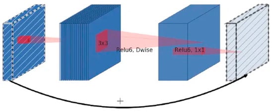
Figure 3.
Inverted residual block.
Although MobileNet V2 improves the feature extraction ability through the inverse residual structure, reduces the loss of low-dimensional features through the linear bottleneck, and the width factor can also be customized to adjust the parameter size of the model, good results have been achieved on the ImageNet dataset. However, in facial expression recognition tasks, the similarity among faces leads to much smaller inter-class differences compared to those in the ImageNet dataset. When using the MobileNet V2 model for face expression recognition, the feature extraction is relatively blind and the feature validity is relatively low, and there is insufficient ability to extract spatial and dimensional information hidden in the features, the network model complexity and loss function can be further improved for the application of facial expression, so as to have a faster speed and higher accuracy in the application of facial expression. In this paper, a novel lightweight network, LightExNet, is proposed based on the MobileNet V2 architecture and tailored to the specific characteristics of facial expression data and classification tasks.
2.2. Details Structure of LightExNet
2.2.1. Overall Network Architecture
In this paper, the facial expression recognition task is divided into 7 categories, and the input image size is fixed at 224 × 224 × 3. This article refers to the MobileNet v2 framework and proposes a lightweight network LightExNet that is more suitable for facial expression features. In order to fully extract original image information, LightExNet is structured as a network based on deep and shallow feature fusion. The network structure is dedicated to fully extracting the shallow features of different scales in the original image and fusing them with the deep features, and then further extracting the useful information in the image through embedding channel and the spatial attention mechanism, and in the final classification process, according to the characteristics of the classification of face expression recognition, an improved central loss function is used to further improve the accuracy of the classification results, and at the same time the loss function adopts the corresponding measures to reduce the amount of computation. Through extensive experimentation and iterative refinement, we have established the final LightExNet architecture as shown in Figure 4.

Figure 4.
The structure of LightExNet.
In the structure diagram, the left part is the data processing flowchart of the whole network, the middle part is the specific operation process and parameters of STAGE0~STAGE5 and AuxSTAGE1~4, and the right part is the data processing flowchart of two types of Bottleneck. Among them, the six links of STAGE0~STAGE5 mainly refer to the backbone network of the lightweight network MobileNet V2, and the four links of AuxSTAGE1~4 use the DW (Depthwise Convolution) convolution and PW(Pointwise Convolution) convolution, respectively, to scale the input original image to four different sizes to form four shallow networks, and to obtain four shallow feature maps with different scales , , , . The four shallow feature maps are then superposed with four deep feature maps of the same size in the backbone network: , , , and , respectively, in the channel dimension. Then four deep and shallow feature fused feature maps are generated: , , , and . This architecture performs channel-wise superposition of deep and shallow feature maps rather than simple element-wise addition. This approach not only preserves shallow-level features from the original input (minimizing information loss) but also mitigates gradient vanishing issues associated with increasing convolutional depth. Furthermore, since deep layers exhibit larger receptive fields while shallow layers retain finer details, this design inherently enables multi-scale feature fusion. To further enhance feature extraction from the cascaded outputs, we introduce a novel dual attention mechanism (channel and spatial), denoted as the “Attention Process” module in the structural diagram.
According to the network architecture diagram of LightExNet, the processing flow of data from input (3 channels of 224 × 224 facial expression images) to output (probability of 7 classification results) is as follows:
- STAGE0: The network accepts a 224 × 224 RGB facial expression image as input, which undergoes initial processing through a standard convolutional operation. In this standard convolution, the convolution kernel is 3 × 3, the step size is 2, and the output channel is 16 (the number of channels in MobileNetV2 is 32, and the results of the analysis of MobileNet V3 have been taken into account, the classification accuracy of the channel number set as 16 and 32 is almost the same in this stage, but it can reduce the computational complexity of the entire classification process to a certain extent). The output results are normalized, and the activation function is RELU6, and the final output is 112 × 112 feature data of 16 channels.
- STAGE1: The 112 × 112 feature data of 16 channels output from STAGE0 is first input into the BTNK1 module (with parameters 16, 112, 1, 16) for processing. As illustrated in the upper-right section of the architecture diagram, the BTNK1 module’s data flow closely follows the step-1 inverted residual block design from MobileNetV2, maintaining its fundamental operational characteristics. The input parameter C is the number of channels of the input data, W is the size of the input data (here the default height size and width size of the input data are the same), T is the expansion factor of the inverted residual structure, and C1 is the depth of the output feature matrix. If C and C1 are the same, the result after linear activation will be added to the input to form the final output result. Otherwise the module’s output undergoes linear activation without adding to the input.
After BTNK1, the feature data size is 16 × 112 × 112 (16 channels, height is 112, and width is also 112), and then input data to the BTNK2 module (parameters 16, 112, 6, 18) for processing, the detailed flow of the BTNK2 module is shown in the lower right of the structure diagram, and its flow is basically the same as that of the inverted residual module with a step size of 2 in MobileNet V2. The meaning of the input parameters here is similar to that of the input parameters in the BTNK1 module. Here the data output from BTNK2 is the first deep feature map with the size of 18 × 56 × 56.
At the same time, the system input tensor (3 × 224 × 224) undergoes processing through the AuxSTAGE1 module to form the first shallow feature map with the size of 6 × 56 × 56. The first deep feature map and the first shallow feature map are cascaded in the channel dimension to form the first deep and shallow fusion feature map with the size of 24 × 56 × 56. This feature matrix is then subjected to the “Attention Process” module (consisting of the channel attention mechanism and the spatial attention mechanism, principles of the mechanism is described in detail later), ultimately generating a 24 × 56 × 56 feature matrix as the final output.
- STAGE2: Following the Attention Process module, the output is a feature matrix of size 24 × 56 × 56, which is firstly input into the BTNK2 module (with the parameters 24, 56, 6, 24) for processing to form an output feature matrix of size 24 × 28 × 28, and then input the data to the BTNK1 module (parameters are 24, 28, 6, 24) for processing to form an output feature matrix with the size of 24 × 28 × 28, which is the second deep feature map .
At the same time, the first shallow feature map from the AuxSTAGE1 module is processed by the AuxSTAGE2 module to form the second shallow feature map with dimensions of 8 × 28 × 28. The second deep feature map and the second shallow feature map are cascaded in the channel dimension to form the second deep and shallow fusion feature map with dimensions of 32 × 28 × 28. Then this feature matrix is processed by “Attention Process” module, and finally a feature matrix with size of 32 × 28 × 28 will be output.
- STAGE3: Following the Attention Process module, the output is a feature matrix of size 32 × 28 × 28, which is firstly input into the BTNK2 module (with the parameters of 32, 28, 6, 48) for processing to form an output feature matrix of size 48 × 14 × 14, and then input into the BTNK1 module (with the parameters of 48, 14, 6, 48) for processing to form an output feature matrix with the size of 48 × 14 × 14, and then input the data to an identical BTNK1 module (with parameters 48, 14, 6, 48) for processing to form an output feature matrix with the size of 48 × 14 × 14 in the end, which is the third deep feature map .
At the same time, the second shallow feature map from AuxSTAGE2 module is processed by AuxSTAGE3 module to form the third shallow feature map with the size of 16 × 14 × 14. The third deep feature map and the third shallow feature map are cascaded in the channel dimension to form the third deep and shallow fusion feature map with the size of 64 × 14 × 14. Then this feature matrix will be processed by “Attention Process” module, and the final feature matrix with the size of 64 × 14 × 14 will be output.
- STAGE4: Following the Attention Process module, the output is a feature matrix with the size of 64 × 14 × 14, which is first input into the BTNK1 module (with the parameters of 64, 14, 6, 96) for processing to form an output feature matrix with the size of 96 × 14 × 14, and then input into another BTNK1 module (with the parameters of 96, 14, 6, 96) for processing to form an output feature matrix with the size of 96 × 14 × 14, and another identical BTNK1 module (with parameters 96, 14, 6, 96) is input for processing to form another output feature matrix with the same dimensions 96 × 14 × 14. Following input the data to another BTNK2 module (with parameters 96, 14, 6, 120) for processing, forming an output feature matrix with the size of 120 × 7 × 7, and then another BTNK1 module (with parameters 120, 7, 6, 120) for processing, finally forming an output feature matrix with the size of 120 × 7 × 7, this is the fourth deep feature map .
At the same time, the third shallow feature map from AuxSTAGE3 module is processed by AuxSTAGE4 module to form the fourth shallow feature map with the size of 40 × 7 × 7. The fourth deep feature map and the fourth shallow feature map are cascaded in the channel dimension to form the fourth deep and shallow fusion feature map with the size of 160 × 7 × 7. Then this feature matrix will be processed by “Attention Process” module, and the final feature matrix with the size of 160 × 7 × 7 will be output.
- STAGE5: Following the Attention Process module, the output is a feature matrix with the size of 160 × 7 × 7, which is first fed into the BTNK1 module (with the parameters of 160, 7, 6, 320) for processing, forming an output feature matrix with the size of 320 × 7 × 7, then after an standard convolution process (convolution kernel is 1 × 1, the number of output channels is 1280, the step size is 1, normalization is performed, the activation function is RELU6, which is actually a fully-connected layer), the feature matrix with the size of 1280 × 7 × 7 is output, and then carry out a mean pooling process (pooling window size is 7 × 7, the step size is 1), the feature matrix with the size of 1280 × 1 × 1 is output. Then the output is processed by an standard convolution (convolution kernel is 1 × 1, the number of output channels is 7, the step size is 1, in fact, here is also a fully-connected layer), and then connected to the improved central loss function, the probability of 7 classification results is output finally.
2.2.2. Channel Attention Module
In convolutional neural networks, each channel in the feature map functions can be regarded as a specialized feature detector. It is possible to give them a weight, giving more attention to the important channels and less to the relatively useless channels, which can improve the feature extraction capability of the network. In order to efficiently compute channel attention, the global spatial information within each channel needs to be compressed into a single channel descriptor. Traditional methods usually use only average pooling to compress spatial information, and study [40] demonstrates that a combination of tied pooling and maximum pooling can be used to infer channel attention in a more fine-grained way. Additionally, most of the current channel attention modules summarize the spatial information by violent encoding, i.e., the size of the feature map is compressed directly from (where denotes the number of channels of the feature map, denotes the height, denotes the width) to , which has the advantage of simplicity, but also inevitably loses more information. To address this limitation, we proposes a novel channel attention module based on the two-step method, which can encode the spatial features more finely, and insert them into the deep and shallow feature fusion, in order to pay attention to those channels with larger gains and suppress irrelevant features.
The proposed channel attention module is shown in Figure 5. Unlike existing methods, this method aggregates spatial information in two steps. The spatial information of the feature maps is first aggregated by average pooling and maximum pooling to different dimensions to retain more spatial information. The feature maps are first compressed to and size by average pooling, and similarly compressed to and size by maximum pooling, in which the spatial information retained by average pooling and maximum pooling to feature maps with the size of is 9 times more than that of the feature maps with the size of , so as to facilitate further learning of spatial features. Then the two types of feature maps with the size of are convolved with 3 × 3 depth-separable convolution to generate two feature maps, and the four feature maps are summed element by element. In order to reduce the number of parameters, the convolution kernel of the depth-separable convolution is shared for each feature map. The merged feature maps are subsequently normalized through sigmoid activation, and each channel descriptor is compressed to the range of 0 to 1, that is, the channel attention map is obtained. The channel attention is calculated as Formula (2):
where: denotes the depth-separable convolutional kernel. denotes the input feature map; denotes the activation function. Finally, we need to multiply the input feature map with the obtained channel attention map to get the weighted feature map, which is calculated as follows Formula (3):

Figure 5.
Channel attention module. In the figure, the green represents the input feature map, the red indicates the 3 × 3 average pooling branch, the purple represents the 3 × 3 max pooling branch, the dark blue corresponds to the 1 × 1 max pooling branch, and the yellow denotes the 1 × 1 average pooling branch.
In the Formula (3) denotes element-by-element multiplication.
2.2.3. Spatial Attention Module
In the facial expression recognition task, the features that are meaningful for expression classification are mainly concentrated on the key parts such as eyebrows, eyes, nose, and mouth, this is due to the fact that these positions contain more texture information, and the features (such as gradient and grayscale, etc.) of these positions will change drastically when a person makes different expressions, so the weight of these key parts can be increased in the feature map by the spatial attention module, which makes the network focus more on the features that are crucial for expression recognition and improve the feature extraction ability of the network. The features of different parts (e.g., eyes, nose, mouth, etc.) may exist in different sizes of receptive fields, and according to the different proportions of the face in the input image, the texture features will also exist in different sizes of receptive fields, if the receptive field is too small, only local features can be observed, and if the receptive field is too large, too much ineffective information is obtained. To address this, we integrate multi-scale feature extraction with spatial attention mechanisms, which can extract weighted features more robustly than single-scale attention.
Figure 6 shows the spatial attention module proposed in this paper. We combines multi-scale feature extraction with spatial attention, which can compute the spatial attention map more finely. In order to calculate the spatial attention, it is first necessary to aggregate the channel information and encode the input feature map into a spatial descriptor in the channel dimension, and we adopts maximum pooling and 3 × 3 convolution to realize this operation. First, the input feature map is maximally pooled to form a maximally pooled layer feature map , and then the input feature map is input into a convolutional layer with a convolutional kernel size of , in order to extract the features in the sensory field of convolutional kernel with the size of . To preserve edge information during convolution operations, we employ zero-padding with a single-pixel border around the feature map boundaries, and the size of the feature map obtained after the convolution is , so the size of output feature maps obtained from the maximally pooled layer and the 3 × 3 convolution layer is same, i.e., , . Combine and in the channel direction to generate an effective feature description, and then use a 7 × 7 convolution kernel (the feature map boundary needs to be filled with 3 layers to avoid losing edge information) for convolution calculation to obtain a spatial attention feature vector with a size of . Finally, the resulting feature vector undergoes nonlinear transformation via sigmoid activation, compressing each spatial feature descriptor to a range of 0–1, and finally outputting the spatial attention feature map . At last, the spatial attention map is used as a weight and multiplied element by element with each channel of the input feature map to obtain the final weighted feature map. The spatial attention calculation method is shown in Formula (4).
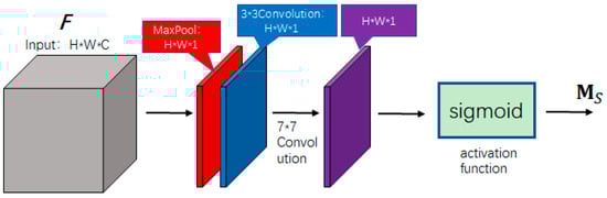
Figure 6.
Spatial attention module. In the figure, gray represents the input feature map, red indicates channel-wise max pooling, blue denotes the 3 × 3 convolution, and purple represents the output after the 7 × 7 convolution. “*” indicates the combination of different dimensions.
In Formula (4), represents the convolution kernel; represents input feature maps; represents the activation function. For the spatial attention module, its input is the output of the channel attention module . Therefore, the calculation formula for the output of the spatial attention module, that is, the output of the entire attention module , is shown in Formula (5):
In Formula (5), denotes element-by-element multiplication. A brief flowchart of the improved attention mechanism module is shown in Figure 7.
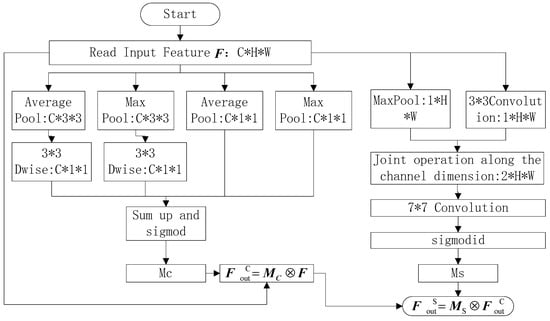
Figure 7.
Improved attention mechanism flowchart. In the figure, “*” indicates the combination of different dimensions.
2.2.4. Stacked Center Loss Function
After the feature maps are processed by the network, they are usually computed directly using the cross-entropy loss function, as shown in Formula (6):
In Formula (6): is the output of the sample before entering the FC layer (the last convolutional layer of the network is actually a FC layer), which belongs to the category . denotes the weight parameter of FC layer . is the size of the batch in a training. denotes the number of categories.
To enhance intra-class feature compactness and inter-class discriminability, we augment the standard cross-entropy loss with center loss, and the center loss calculation process is shown in the Formula (7):
In Formula (7), is the feature center of category . When the category training is updated, in order to avoid the new center jittering too much, the momentum mechanism is introduced, which makes the update of the category center smoother and reduces the impact of a single sample update on the center. The update of the category center is no longer completely dependent on the features of the current batch of samples, but combines the center position of the previous round and the adjustment amount of the current batch, as shown in Formula (8):
In the Formula (8), is the center of category at the iteration . is the adjustment amount of the current batch to the center. is the momentum coefficient (usually taken as 0.5–0.9, with a value of 0.5 at the beginning of training (the first 50% of epoch) to quickly approximate the real center, and gradually increasing to 0.9 at the end of training (the last 50% of epoch) to stabilize the center position), which controls the degree of update smoothing. This approach significantly mitigates training instability while demonstrating enhanced robustness to noisy samples and label outliers.
In facial expression recognition tasks, the use of an improved central loss function is aimed at improving the classification performance and generalization ability of the model, but at the same time, it also introduces additional computational overhead, generally increasing training time by about 10% to 20%. However, the specific proportion of computational increase that will result depends on multiple factors, making this consideration particularly critical for lightweight models where resource constraints are paramount. In order to alleviate the additional computational burden caused by the central loss function, the following measures have been taken in this paper:
- Low-frequency update: reduce the update frequency of , in this paper updates once every three iterations.
- Asynchronous updates: even with low-frequency updates, instead of updating the centers of all categories with each update, updates are made only for those categories that appear in the current batch.
Finally, the overall loss function equation is:
In Formula (9), denotes the central loss coefficient, which is used to control the proportion of the loss function. In this paper, the value of is carefully adjusted after many experimental optimizations, and finally the value of 0.03 is taken in the first 50% of the epoch to strengthen the feature aggregation, and the value of 0.008 is taken in the last 50% of the epoch to maintain the classification accuracy.
The algorithm of the stacked center loss function module is as follows:
# Initialize class centers c[j] as zero vectors (j = 1…num_classes)
For each class j in [1, num_classes]:
c[j] ← ZeroVector(feature_dim)
# Training loop
For each epoch in total_epochs:
# Dynamically adjust momentum coefficient beta and center loss weight lambda
If epoch < total_epochs * 0.5:
beta ← 0.5
lambda_center ← 0.03
Else:
beta ← 0.9
lambda_center ← 0.008
For each iteration t in epoch:
# Get current batch samples and labels
batch ← SampleBatch()
features ← ExtractFeatures(batch.inputs) # Feature representations
logits ← FinalLayer(features) # Output logits
labels ← batch.labels
B ← batch.size
# Compute cross-entropy loss
loss_ce ← CrossEntropy
# Compute center loss
loss_center ← 0
For i in [1, B]:
j ← labels[i]
loss_center +=1/2*|| features[i] − c[j] ||^2
loss_center ← loss_center/B
# Total loss
loss_total ← loss_ce + lambda_center * loss_center
# Backpropagation and model parameter update
Backpropagate(loss_total)
UpdateModelWeights()
# Update class centers every 3 iterations (low-frequency update)
If t mod 3 == 0:
# Get the set of active classes in the current batch (asynchronous update)
active_classes ← Unique(labels)
For each class j in active_classes:
# Find all samples belonging to class j
samples_j ← { features[i] | labels[i] == j }
# Compute the mean feature vector delta for class j
delta ← Mean(samples_j)
# Update class center using momentum-based smoothing
c[j] ← beta * c[j] + (1 − beta)* delta
2.2.5. Comparison with MobileNet V2
Compared with the original MobileNet V2 architecture, LightExNet introduces several targeted improvements to better suit the task of facial expression recognition:
- Deep-Shallow Feature Fusion: In LightExNet, four auxiliary branches extract shallow features at different scales from the original image, which are then fused with corresponding deep features from the backbone network in the channel dimension. This design preserves local texture information and enhances robustness to subtle facial variations.
- Improved Attention Mechanism: A lightweight yet effective attention module is added after each feature fusion stage. It combines channel and spatial attention to dynamically highlight important facial regions (e.g., eyes, mouth), thus improving discriminative feature learning without adding significant computational overhead.
- Stacked Center Loss: In addition to the standard cross-entropy loss, an improved center loss function is adopted to enforce intra-class compactness and inter-class separability. To maintain the model’s efficiency, the center loss is updated with a low-frequency and asynchronous strategy.
- Computational Efficiency: Despite these enhancements, LightExNet maintains a lightweight nature with slightly fewer parameters and FLOPs than MobileNet V2 (3.27 M vs. 3.5 M, 298.27 M vs. 312.86 M), while achieving significantly higher recognition accuracy across benchmark datasets.
These improvements are summarized visually in Figure 4, where the modified modules and structural differences are clearly highlighted. In Figure 4, the components and labels marked in red indicate the differences between LightExNet and MobileNet V2. Additionally, in LightExNet, for the bottleneck modules in MobileNet V2 where the number of repetitions n is greater than 1, the number of repetitions has been reduced by 1.
3. Experiments and Results
3.1. Data Set Details
The algorithms in the paper are experimentally validated on three public data face expression sets FER2013, CK+ [41] and RAF-DB [42].
The FER2013 (Facial Expression Recognition 2013) dataset is a widely used dataset for facial expression recognition research. The FER2013 dataset was presented by Pierre-Luc Carrier and Aaron Courville at the 2013 ICML (International Conference on Machine Learning) conference. It contains pixel data of face images labeled with 7 basic expression categories. The number of images in the FER2013 dataset is 35,887 grayscale face images, each with a size of 48 × 48 pixels, with a total of seven basic expressions. The FER2013 dataset is divided into three parts, training set: 28,709 images, validation set: 3589 images, and test set: 3589 images. The dataset is provided as a CSV file. Each row of data contains the following information: emotion: expression label (0 to 6, corresponding to 7 expressions), Usage: identifies whether the image belongs to the training set, validation set, or test set (with the value of Training, PublicTest, or PrivateTest), pixels: pixel values of the image, stored as strings, with each pixel value ranging from 0 to 255, each image has 48 × 48 pixel values, and the example data is shown in the Figure 8 (the pixel values of each image are only listed in the first few). The images in the FER2013 dataset are collected from the Internet and contain different lighting conditions, poses, and occlusions. So it is more difficult to recognize them, and there is a category imbalance problem, with a smaller number of samples for some expression categories (e.g., “Disgust” category), and all images are grayscale with no color information.
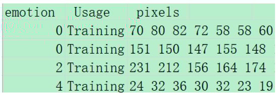
Figure 8.
Example of image data from the FER2013 dataset.
The CK+ (Extended Cohn-Kanade) dataset is one of the most commonly used benchmark datasets in the field of facial expression recognition, developed by the team of Jeffrey Cohn and Takeo Kanade at the University of Pittsburgh, and subsequently extended by Patrick Lucey et al. The original CK dataset was released in 2000, and the extended version, CK+, was released in 2010. The CK+ dataset contains 123 subjects with a total of 593 video sequences of facial expressions, each starting with a neutral expression and progressively transitioning to a peak expression, labeled with seven basic expressions (anger, disgust, fear, happiness, sadness, surprise, and contempt). The image resolutions in the CK+ dataset are 640 × 490 or 640 × 480 pixels and the images are in grayscale format. Due to the high quality of the annotations and the relatively large size of the CK+ dataset, it serves as a benchmark when evaluating new methods. In addition, the dataset is also suitable for studying the link between facial expressions and internal emotional states. The CK+ dataset also has some limitations, such as the limited diversity of participants and the fact that all data were collected in a controlled environment, which may limit the model’s generalization ability in more natural environments. Several sample images of the CK+ dataset is shown in the Figure 9.
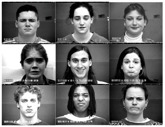
Figure 9.
CK+ dataset sample images.
The RAF-DB dataset was developed by the Institute of Computing Technology (ICT), Chinese Academy of Sciences (CAS) in 2017, with images sourced from the Internet covering different races, ages, lighting conditions, and postures, and containing a total of 29,672 single-labeled emoji images and multi-labeled emoji images. The single-labeled images contain seven types of expression (anger, disgust, fear, happiness, sadness, surprise, and neutral), totaling 15,339 images, which were selected as the dataset. In the single-label image set of RAF-DB dataset, there are 12,271 images in the training set and 3068 images in the test set. Some sample images are shown in Figure 10.
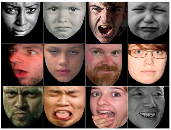
Figure 10.
Sample images from RAF-DB dataset.
For the FER2013 and RAF-DB datasets, we applied a set of data augmentation techniques including random horizontal flipping, random cropping, small-angle random rotation (±10°), and color jittering to increase training sample diversity and improve model generalization. In contrast, for the smaller CK+ dataset, we employed a more conservative augmentation strategy, including random horizontal flipping and light random cropping with minimal color jitter, while avoiding rotation to preserve the subtle expression details.
3.2. Experimental Environment and Configuration
The experiments in this paper are done under Windows 10 operating system. The experimental environment includes basic computer hardware, graphic image processing unit (GPU), central processing unit (CPU), parallel computing library, deep learning framework, Programming languages and Compiler, etc., and the specific experimental environment configuration is shown in the Table 2.
Table 2.
Experimental environment configuration.
There are more hyperparameters involved in the network training process, mainly including: Batch Size, Epochs, initial learning rate, learning decay rate, optimizer, etc. In the experiments of this paper, according to the performance of the GPU, the size of the dataset and the expectation of the model generalization, due to the significantly smaller size of the CK+ dataset compared to FER2013 and RAF-DB, we adopted a smaller batch size (16) and a lower initial learning rate (0.0001) to prevent overfitting and ensure more stable convergence. In contrast, for the larger datasets FER2013 and RAF-DB, a batch size of 32 and an initial learning rate of 0.001 were chosen to accelerate training while maintaining good generalization. According to the size of the training set and the complexity of the model, the Epochs value is set to 150, and the decreasing learning rate is used to make the model easier to converge. The learning rate decay is set as the cosine annealing method, the minimum learning rate is set to 1/100 of the initial learning rate, and the optimizer adopts AdamW optimizer. The specific hyperparameter settings are shown in Table 3.
Table 3.
Hyperparameter setting.
3.3. Experimental Results and Analysis
3.3.1. Experimental Results on the Dataset
To verify the effectiveness of the proposed LightExNet algorithm, experiments were conducted on the FER2013, CK+, and RAF-DB datasets, and the results were visualized.
- Experimental results on the Fer2013 dataset
Figure 11 shows the training accuracy curve obtained by the model on the Fer2013 dataset. By analyzing the picture, it can be concluded that the curve as a whole is rising as the number of iterations stacks up, which means that the accuracy of the training is constantly improving, and continuing the analysis, it can be seen that the training accuracy improves the fastest at the very beginning of the training phase, i.e., before the 21st generation. When training proceeds to about generation 35, the curve rise begins to slow down and the slope begins to gradually decrease. However, at around generation 45, the slope of the curve starts to grow again, and the curve starts to rise faster, and then slows down at generation 70, and then after generation 110, the curve becomes smooth, and the accuracy of the training no longer changes significantly, until it finally converges.
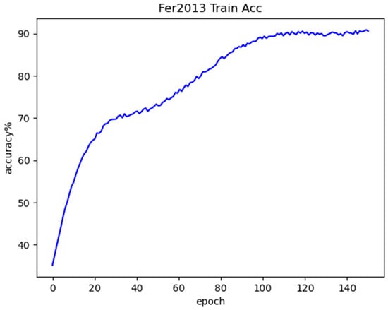
Figure 11.
Fer2013 training accuracy curve.
Figure 12 shows the test accuracy curve. By analyzing the figure, it can be observed that, similar to the training curve, the test accuracy also increases overall with the number of iterations. The most significant improvement occurs during the early training phase, specifically within the first 21 epochs. However, the overall direction of the curve is gradually stabilized, the slope of the curve gradually decreases, and the improvement of the accuracy also slows down gradually, until it eventually stabilizes and reaches the convergence state.

Figure 12.
Fer2013 testing accuracy curve.
The confusion matrix of the Fer2013 test set is shown in Figure 13.

Figure 13.
Fer2013 confusion matrix results.
It is easy to see from Fer2013 confusion matrix results (Figure 13) that the method proposed in this paper has a higher degree of recognition for the two types of expression, Happy and Surprised, compared with other expressions, with an accuracy of 0.89 and 0.87, respectively, but at the same time the recognition rates for the three types of expression, Fear, Anger and Sadness, are relatively lower.
- Experimental results on the CK+ dataset
Figure 14 shows the training accuracy curve obtained by the model on the CK+ dataset, Figure 15 shows the test accuracy curve obtained by the model on the CK+ dataset, and Figure 16 shows the confusion matrix for the CK+ test set. From these figures. It can be seen that there is a great degree of improvement in the recognition accuracy for the seven types of expressions compared to the previous Fer2013 test set, and the recognition accuracy for each type of expression does not vary as much as it did in the Fer2013 dataset, which occurs due to the fact that the CK+ dataset was captured under laboratory conditions, which reduces the environmental and interference of human factors, so the quality of the images can be guaranteed, which is why the model has a more excellent recognition accuracy on the CK+ dataset.

Figure 14.
CK+ training accuracy curve.
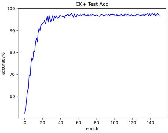
Figure 15.
CK+ testing accuracy curve.
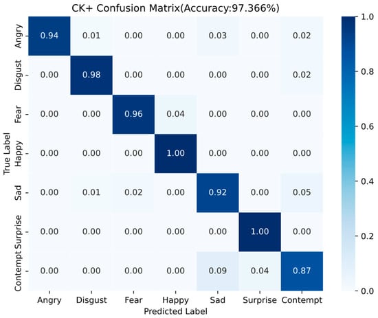
Figure 16.
CK+ confusion matrix results.
The confusion matrix on the CK+ facial expression dataset reveals the detailed recognition performance across seven emotion categories. Overall, the model achieves an impressive accuracy of 97.366%, indicating its strong capability in facial expression recognition tasks.
Among all categories, Happy and Surprise expressions are recognized with perfect accuracy (1.00), Disgust and Fear achieve high recognition rates of 0.98 and 0.96, respectively, with minimal confusion. Angry achieves a recognition rate of 0.94, with a few samples misclassified as Sad and Contempt. Sad obtains a slightly lower accuracy of 0.92, and is most frequently confused with Contempt (0.05). The most challenging category to classify is Contempt, which exhibits the lowest recognition rate of 0.87. It is often misidentified as Sad (0.09) or Surprise (0.04).
- Experimental results on RAF-DB dataset
Figure 17 shows the training accuracy curve obtained by the model on the RAF-DB dataset, Figure 18 shows the test accuracy curve obtained by the model on the RAF-DB dataset, and Figure 19 shows the confusion matrix for the RAF-DB test set. From these figures, it can be seen that in the test curve, the accuracy reaches about 80% when epoch is 20, and before that the accuracy is increasing rapidly with the increase of epoch, and then the accuracy increases slowly with the increase of epoch, and the accuracy basically reaches about 86% of the highest accuracy of the algorithm in predicting the unknown samples when epoch is about 70, and thereafter the accuracy is basically maintained at the highest accuracy of about 86% with the epoch increases. Among them, the recognition rate of Happy expression is the highest at 95%, and Disgust and Fear emojis have the lowest recognition rates, with a 6% probability that a disgust emoji will be misrecognized as an angry emoji and an 10% probability that a fear emoji will be misrecognized as a surprised emoji.
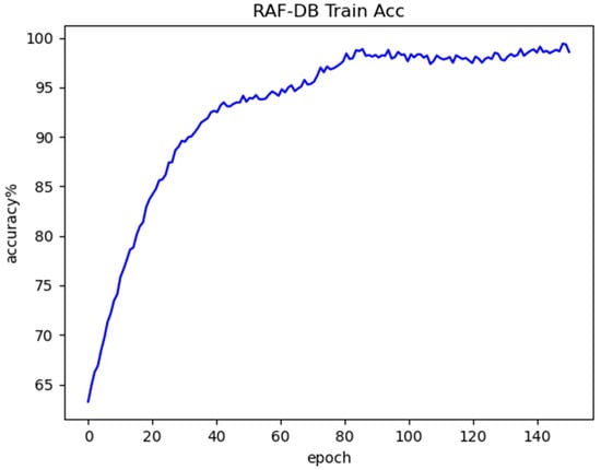
Figure 17.
RAF-DB training accuracy curve.
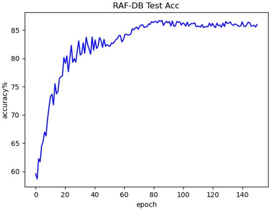
Figure 18.
RAF-DB testing accuracy curve.
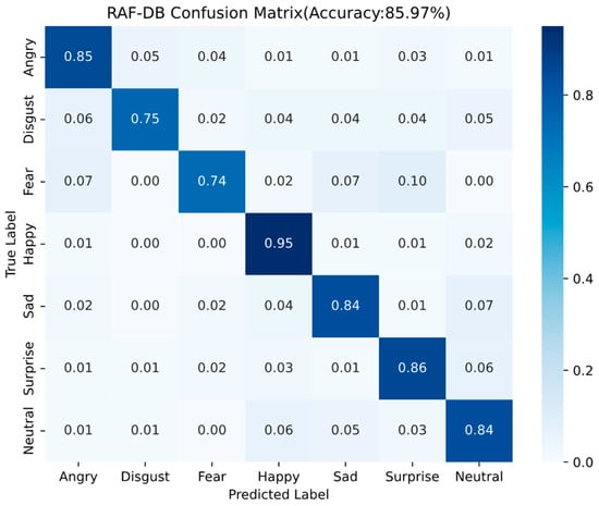
Figure 19.
RAF-DB confusion matrix results.
3.3.2. Comparative Experiment and Analysis
The evaluation of deep learning models extends beyond conventional accuracy metrics to encompass critical computational characteristics, including parameter efficiency and computational complexity, which jointly determine practical deployability. In order to better compare the performance of this paper’s method and the latest face expression recognition algorithms, this paper reproduces some important expression recognition algorithms and extracts their key indexes for comparison experiments. Relevant experiments are conducted on Fer2013, CK+ and RAF-DB datasets, and the results are shown in Table 4 and Table 5. Analyzing Table 5, it can be seen that the proposed method in this paper has the highest accuracy on Fer2013, CK+ and RAF-DB datasets, which are 69.17%, 97.37, and 85. 97%, respectively. Compared with the Improved MobileNet V2 network in study [32] (the Improved MobileNet V2 network in study [32] has further improved the accuracy over the original MobileNet V2 network on all three datasets), the accuracy of this paper’s method on the Fer2013, CK+, and RAF-DB datasets in absolute terms improved by 0.55%, 1.41%, and 2.54%, respectively. The number of parameters is reduced by 6.57% and the computational complexity of the model is reduced by 4.66% compared to the MobileNet V2 network. Compared with recent lightweight expression recognition algorithms IE-DBN [19], Improved Mobilenet V2 [32], Model by Sidhom O et al. [20], Self-Cure Net [21], Improved MobileViT [33], MFN [34], MFN+ [34], Ada-CM [23], Parallel CNN [35], etc. This paper’s method has a smaller number of parameters, moderate model inference time, and the highest accuracy rate. The above experiments verify the effectiveness of this paper’s method for facial expression recognition on faces.
Table 4.
Comparison of parameters of various models.
Table 5.
Performance comparison of various models.
3.3.3. Ablation Experiment
Experiments on the datasets Fer2013, CK+ and RAF-DB with different improvement schemes can verify the effect of each part of the module on the model as a whole, and the experimental results are shown in Table 6. In Table 6, ① stands for deep and shallow feature fusion function, ② stands for channel and spatial attention mechanisms, ③ represents improved center loss function.
Table 6.
Ablation experiment of LightExNet.
Analyzing Table 6, it can be seen that in Scenario 1, the combination of the backbone network Base and the deep and shallow feature fusion module has 3.12 M Params and 286.73 M FLOPs, with an Accuracy of 65.26% on the Fer2013 dataset, 94.73% on the CK+ dataset, and 81.37% on the RAF-DB dataset, which shows that, in order to seamlessly fuse the deep and shallow networks, LightExNet has streamlined the architecture of MobileNet V2. Although the deep and shallow feature fusion module has been added, its Params and FLOPS parameters are still slightly lower than those of MobileNet V2, and the accuracy on the three datasets is basically equivalent to MobileNet V2, which proves the effectiveness of the deep and shallow feature fusion module in face expression recognition.
In Scheme 2, the channel and spatial attention mechanism is added, and its Params and FLOPs are increased to 3.23 M and 294.93 M, respectively, and the Accuracy is 67.96% on the Fer2013 dataset, 96.12% on the CK+ dataset, and 84.34% on the RAF-DB dataset. Comparing with Scheme 1, the model complexity becomes slightly higher, but the recognition accuracy is improved, indicating that the channel and spatial attention mechanism can effectively improve the feature extraction ability of the model.
In Scenario 3, compared with Scenario 1, only the improved central loss function is added, and its Params and FLOPs are slightly increased to 3.16 M and 289.76 M, respectively. The accuracy is 65.97% on the Fer2013 dataset, 95.70% on the CK+ dataset, and 83.11% on the RAF-DB dataset. Comparing with Scheme 1, it can be seen that the improved central loss function can effectively improve the classification performance and generalization ability of the model, and there is no significant increase in Params and FLOPs by the measure of mitigating the extra computational burden brought by the central loss function.
In Scheme 4, both the channel and spatial attention mechanisms, and the improved central loss function are introduced, with Params of 3.27 M, FLOPs of 298.27 M, and the accuracy on the Fer2013 dataset is 69.17%, on the CK+ dataset is 97.37%, and on the RAF-DB dataset is 85.97%, which is still slightly lower in terms of the number of parameters compared to MobileNet V2, but the Accuracy on the three datasets does improve in some ways, proving LightExNet is more suitable for the task of recognizing facial expressions.
To better understand the contribution of each structural component in LightExNet, we conducted an ablation study based on the baseline MobileNet V2 architecture. As shown in Table 7, three key modules were gradually integrated into the backbone.
Table 7.
Effectiveness of Individual Components Compared to Baseline MobileNet V2.
The base model (MobileNet V2) achieves 67.02%, 93.26%, and 81.41% accuracy on FER2013, CK+, and RAF-DB, respectively. When only the feature fusion module (①) is added (Scheme 1), the performance on FER2013 unexpectedly drops, suggesting that shallow features alone may be insufficient without additional attention.
The introduction of the attention mechanism (②, Scheme 2) significantly improves performance across all datasets, with +3.60% accuracy gain on RAF-DB. Adding the center loss module (③, Scheme 3) also enhances generalization, especially on CK+.
The full LightExNet model (Scheme 4) integrates all three components and achieves consistent improvement on all datasets, including a +3.21% gain on FER2013, +4.41% on CK+, and +5.60% on RAF-DB, while reducing parameter count by 6.57% and FLOPs by 4.66% compared to the baseline. This confirms that the proposed components work synergistically to improve both efficiency and effectiveness.
3.4. Inference Evaluation of LightExNet on Mobile Device
To validate the real-world deployment capability of the proposed LightExNet model, we conducted a direct on-device comparison with the standard MobileNet V2 model using the PyTorch Mobile framework on a representative mid-range Android smartphone—Redmi Note 13 5G. LightExNet is specifically designed for lightweight expression recognition, incorporating deep–shallow feature fusion, a stacked attention mechanism, and a center loss-based optimization strategy, all of which aim to improve discriminative capacity with minimal computational overhead. Device and deployment details are shown in Table 8.
Table 8.
Device and deployment details.
To better assess the practical inference efficiency and deployment readiness of the proposed LightExNet model, we conducted a direct comparative evaluation against the standard MobileNet V2 architecture. Both models were trained using PyTorch under consistent settings and exported to TorchScript format (.pt) for mobile deployment.
The two models were then deployed on the Redmi Note 13 5G smartphone using the PyTorch runtime, and inference was performed directly on-device using single-frame inputs of the same resolution (224 × 224). The testing environment was kept consistent for both models, including preprocessing operations, runtime conditions, and input sources, ensuring a fair and controlled comparison.
Performance metrics such as inference latency, frame rate, memory usage, power consumption, and classification accuracy were measured and averaged across multiple runs. The following table presents the comparative results of LightExNet and MobileNet V2 under identical mobile deployment settings.
Performance comparison of two algorithms is shown in Table 9.
Table 9.
Performance comparison of LightExNet and MobileNet V2.
This mobile inference evaluation demonstrates that LightExNet achieves a better trade-off between recognition accuracy, runtime performance, and model size than MobileNet V2 on a representative mid-tier Android device. The results confirm the effectiveness of the proposed architecture for practical mobile deployment, satisfying the real-time requirements of edge-side applications such as human-computer interaction, smart terminals, and mobile health monitoring.
4. Discussion
The comprehensive experimental results across the FER2013, CK+, and RAF-DB datasets highlight both the strengths and limitations of the proposed LightExNet framework in facial expression recognition (FER). The model consistently outperforms several state-of-the-art lightweight FER methods in terms of classification accuracy, parameter efficiency, and computational complexity, underscoring its effectiveness in real-world, resource-constrained applications.
4.1. The Reasons for the Variations in Recognition Accuracy Across Different Facial Expressions
4.1.1. Fer2013 Dataset
The performance discrepancy of Fer2013 dataset arises because happy and surprised expressions in the FER2013 dataset exhibit more distinctive facial features compared to other emotion categories, enabling superior feature extraction and consequently higher recognition accuracy by the neural network. The facial expression images of faces in the happy state tend to have clearly distinguishable feature information such as the corners of the mouth are raised and lines are created at the corners of the eyes. Face expressions in the state of surprise will also show obvious expression features such as eyes widening and mouth opening. In comparison, the recognition rates of the fear, anger and sadness expressions are relatively low. Fear is the most difficult to recognize, because in the fear expression, there is also the case of mouth opening, only that the mouth opening amplitude is slightly larger, which leads to easy confusion between the two categories of fear and surprise, and at the same time, it is easy to be confused with the sadness category, because there are frowning, forehead tightening, and other similar features in the two categories, so the recognition rate of the fear category of facial expressions is the lowest among all the categories. The remaining two categories of expressions and the fear category are all negative emotional expressions, and there is a strong similarity between the features of the three categories, and the difference between the facial key points is usually very small, which leads to a high probability of confusion, thus resulting in a relatively low recognition accuracy rate for these three categories of expressions.
4.1.2. CK+ Dataset
Happy and Surprise expressions are recognized with perfect accuracy (1.00), likely due to their distinct facial features, such as pronounced mouth curvature and wide-open eyes, which make them easily distinguishable from other expressions.
Fear is occasionally misclassified as Happy or Sad, which may be attributed to overlapping facial cues such as widened eyes or tension in the eyebrows.
Angry has a few samples misclassified as Sad and Contempt. This confusion can be explained by the shared facial characteristics among these expressions, such as furrowed brows and downward lip movement.
Sad often confused with Contempt (0.05), possibly due to the subtle and nuanced facial muscle movements involved in expressing sadness, which overlap with negative valence expressions like contempt and fear.
Contempt is often misidentified as Sad (0.09) or Surprise (0.04). This result may stem from the subtlety and asymmetry typically associated with contemptuous expressions (e.g., unilateral lip raise), making them harder to distinguish. Additionally, the relatively limited number of contempt samples in the CK+ dataset may further contribute to the lower classification accuracy.
4.1.3. RAF-DB Dataset
The recognition rate of Happy expression is the highest mainly due to the fact that the happy label has the largest number of images, possesses rich expression features, and is easy to distinguish from other expressions. Disgust and Fear emojis have the lowest recognition rates, and Disgust emoji is easy misrecognized as an Angry emoji, Fear emoji is easy misrecognized as a surprised emoji. This is due to the fact that these expressions share highly similar regional features, making them easy to confuse.
4.2. Generalization Across Datasets
LightExNet achieves the highest overall accuracy on all three datasets compared to a variety of baseline and advanced FER models. On the controlled CK+ dataset, which features high-quality, laboratory-captured images, the model attains a remarkable 97.37% accuracy. This performance illustrates the model’s capacity to leverage clean data for precise expression recognition. On the more challenging, in-the-wild RAF-DB and the class-imbalanced FER2013 datasets, the model still achieves competitive accuracies of 85.97% and 69.17%, respectively. These results confirm that LightExNet generalizes well across domains with varying degrees of noise, occlusion, and class balance.
4.3. Impact of Dataset Characteristics
The observed differences in performance across datasets can be largely attributed to the quality and distribution of the data. For instance, the FER2013 dataset exhibits substantial class imbalance and contains low-resolution, noisy images. This results in skewed performance favoring dominant classes like Happy and Surprise, with poor recognition for underrepresented or ambiguous emotions such as Fear and Disgust. Conversely, the CK+ dataset benefits from well-balanced class representation and consistent image quality, leading to more uniform accuracy across emotion categories. RAF-DB, although collected in unconstrained environments, still provides clearer facial cues and more diverse expressions than FER2013, which contributes to its intermediate performance range.
4.4. Effectiveness of Architectural Enhancements
Ablation studies provide empirical support for the contribution of each architectural component. The fusion of deep and shallow features not only maintains a low parameter count (3.12 M) but also enhances early-stage detail retention, which is particularly beneficial for recognizing subtle expressions. The addition of the channel-spatial attention mechanism further boosts accuracy (up to 96.12% on CK+) by allowing the network to dynamically focus on informative regions of the face. Meanwhile, the integration of an improved center loss function leads to better class separability in the embedding space, especially for visually similar emotions such as Fear and Sad, with minimal computational overhead. When all three components are combined, LightExNet achieves its best performance, demonstrating that these modules synergistically enhance both discriminative power and generalization.
4.5. Efficiency vs. Accuracy Trade-Off
LightExNet strikes a favorable balance between recognition accuracy and model efficiency. Compared with the baseline MobileNet V2 and several other compact models, it achieves higher accuracy while reducing parameter count (3.27 M vs. 3.5 M) and FLOPs (298.27 M vs. 312.86 M). This makes it well suited for deployment in edge-computing scenarios such as mobile devices or embedded systems, where memory and power constraints are critical considerations.
4.6. Limitations and Future Directions
Although LightExNet achieves competitive performance on Fer2013, CK+, and RAF-DB, there are several directions to further enhance its robustness and practicality:
- Limitations on Imbalanced Datasets
Despite the overall effectiveness of the proposed model, certain limitations remain, particularly when applied to datasets with highly imbalanced class distributions such as FER2013. As illustrated in the confusion matrix, the recognition performance varies significantly across emotion categories. Emotions with more training samples, such as Happy, Surprise, and Neutral, achieve relatively high accuracy (e.g., 0.89, 0.87, and 0.74, respectively). In contrast, underrepresented classes such as Fear and Sad exhibit lower accuracy (0.51 and 0.57), and Disgust is frequently misclassified as Angry (19%) or Fear (5%).
These results suggest that the model tends to be biased toward majority classes, which is a common issue in deep learning when trained on imbalanced data. To address this limitation, future work could explore strategies such as oversampling of minority classes, use of class-balanced loss functions (e.g., focal loss), or synthetic data augmentation techniques to improve the representation of underrepresented emotions. Additionally, transfer learning from more balanced or diverse datasets may help enhance the model’s generalizability across emotion categories.
- Extended Dataset Evaluation
The current experiments focus on three mainstream datasets, but testing on larger and more diverse datasets (e.g., AffectNet for in-the-wild expressions, or JAFFE for cross-cultural analysis) would better validate the model’s generalization ability. Future work will include these datasets and investigate domain adaptation techniques to address potential distribution shifts.
- Loss Function Optimization
While the improved center loss in LightExNet effectively enhances feature discrimination, other advanced loss functions (e.g., ArcFace for angular margin optimization or adaptive weight-based losses for imbalanced data) could further refine intra-class compactness. A comparative study of these losses will be conducted to balance accuracy and computational cost.
- Sensitivity to Occlusion:
The current model is trained primarily on datasets with relatively clean facial images. In scenarios involving partial occlusion (e.g., masks, hands, glasses), the model’s accuracy may degrade due to the loss of critical facial features. Future work may incorporate occlusion-aware training strategies or synthetic occlusion augmentation to improve robustness.
- Non-Frontal Pose Handling:
The model assumes near-frontal facial alignment for optimal performance. Although some degree of pose variation is tolerated, performance may decrease on non-frontal or profile views. Integrating pose normalization or multi-view learning could help address this issue.
- Real-Time Constraints in Ultra-Low-End Devices:
Although LightExNet performs well on mid-tier devices (e.g., Redmi Note 13 5G), its inference time may not fully meet real-time requirements on extremely resource-constrained platforms such as entry-level microcontrollers or legacy smartphones without GPU/NPU support. Future improvements may consider model quantization or dynamic computation strategies.
In summary, LightExNet demonstrates strong performance in static image-based FER tasks, offering a compelling trade-off between accuracy and computational efficiency. The results validate the proposed architectural innovations and provide a solid foundation for future enhancements aimed at broader deployment and improved robustness across complex real-world scenarios.
5. Conclusions
Compared to other lightweight convolutional neural networks, MobileNet V2 is well suited for facial expression recognition. However, it still suffers from several issues, such as feature extraction is relatively blind so the effectiveness of features is relatively low, and the ability to extract spatial and dimensional information hidden in the features is insufficient, etc. In this paper, we propose LightExNet, a lightweight network built upon MobileNet V2, specifically designed to address these challenges in facial expression recognition.
In LightExNet, the deep and shallow feature fusion is firstly fused, in which the deep and shallow feature maps are superposed in the channel dimension rather than simply summed up, which can not only fully extract the shallow features in the original image and reduce the information loss, but also can alleviate the problem of gradient disappearance when the number of convolutional layers increases. Additionally, the sensory field of the deep network is relatively large, and the sensory field of the shallow network is relatively small, and this structure can also achieve the effect of multi-scale feature fusion. At the same time, we streamline the MobileNet V2 architecture to better integrate the deep and shallow networks, facilitating seamless fusion. In addition, in order to more effectively extract the useful information contained in the cascaded feature map, a new channel and spatial attention mechanism is proposed. Based on fully extracting the features of the expression itself, and, as far as possible, obtaining the feature information of different expression regions for encoding, so as to improve the accuracy of expression recognition. In the final classification process, according to the characteristics of face expression recognition classification, the improved center loss function is superimposed to further improve the accuracy of the classification results, and, at the same time, corresponding measures were taken to reduce the computational complexity of the joint loss function.
LightExNet is evaluated on three benchmark datasets: Fer2013, CK+, and RAF-DB. The experimental results show that the Parameters of LightExNet is 3.27 M, the Flops is 298.27 M, and the accuracy is 69.17%, 97.37%, and 85.97% on the three datasets, respectively, and the comprehensive performance is better than the current mainstream lightweight expression recognition algorithms such as MobileNet V2, IE-DBN, Self-Cure Net, Improved MobileViT, MFN, Ada-CM, Parallel CNN etc. So LightExNet is proved to have greater application value and potential in the field of lightweight expression recognition.
Author Contributions
Conceptualization, Q.Y. and Y.H.; methodology, Q.Y. and Y.H.; software, Q.Y., Y.H. and Z.R.; validation, Q.Y.,Y.H. and Y.W.; formal analysis, Z.R. and H.C.; investigation, Y.W.; resources, Y.H. and H.C.; data curation, Y.W.; writing—original draft preparation, Q.Y.; writing—review and editing, H.C. and Y.W.; visualization, H.C.; supervision, Y.H.; project administration, Z.R.; funding acquisition, Y.H. and Q.Y. All authors have read and agreed to the published version of the manuscript.
Funding
This research was funded by: Research on Key Technologies of Robot Vision Perception and Agile Operation for 3C Manufacturing, Jiangxi Province 03 special projects and 5G projects, grant number 20232ABC03A09. Research on the Application of Data Mining in Supporting Decision-Making for the Prediction of Sandstone-Type Uranium Mineralization, Science and Technology Research Project of Jiangxi Provincial Department of Education, grant number GJJ180379. Research on Machine Learning-based Multi-source Heterogeneous Data Cleaning Techniques for Nuclear Geosciences, Jiangxi Engineering Technology Research Center of Nuclear Geoscience Data Science and System, Open Fund Program, grant number JETRCNGDSS201803.
Data Availability Statement
Our datasets (FER2013, CK+, and RAF-DB) are all public datasets. The datasets (FER2013, CK+, and RAF-DB) used in this study are publicly available from https://www.kaggle.com/datasets/deadskull7/fer2013 (accessed on 13 December 2023), https://www.kaggle.com/datasets/davilsena/ckdataset (accessed on 12 December 2023), and https://gitcode.com/open-source-toolkit/77641 (accessed on 11 December 2024). Further inquiries can be directed to the corresponding author.
Conflicts of Interest
The authors declare no conflicts of interest.
References
- Li, S.; Deng, W. Deep Facial Expression Recognition: A Survey. IEEE Trans. Affect. Comput. 2022, 13, 1195–1215. [Google Scholar] [CrossRef]
- Ekman, P.; Friesen, W.V. Constants across cultures in the face and emotion. J. Pers. Soc. Psychol. 1971, 17, 124–129. [Google Scholar] [CrossRef] [PubMed]
- Liu, W.; Zhou, L.; Chen, J. Face Recognition Based on Lightweight Convolutional Neural Networks. Information 2021, 12, 191. [Google Scholar] [CrossRef]
- Sajjad, M.; Zahir, S.; Ullah, A.; Akhtar, Z.; Muhammad, K. Human Behavior Understanding in Big Multimedia Data Using CNN based Facial Expression Recognition. Mob. Netw. Appl. 2020, 25, 1611–1621. [Google Scholar] [CrossRef]
- Chowdary, M.K.; Nguyen, T.N.; Hemanth, D.J. Deep learning-based facial emotion recognition for human–computer interaction applications. Neural Comput. Appl. 2021, 35, 23311–23328. [Google Scholar] [CrossRef]
- Khaireddin, Y.; Chen, Z. Facial Emotion Recognition: State of the Art Performance on FER2013. arXiv 2021, arXiv:2105.03588. [Google Scholar]
- Minaee, S.; Minaei, M.; Abdolrashidi, A. Deep-Emotion: Facial Expression Recognition Using Attentional Convolutional Network. Sensors 2021, 21, 3046. [Google Scholar] [CrossRef]
- Schoneveld, L.; Othmani, A.; Abdelkawy, H. Leveraging Recent Advances in Deep Learning for Audio-Visual Emotion Recognition. Pattern Recognit. Lett. 2021, 146, 1–7. [Google Scholar] [CrossRef]
- Krizhevsky, A.; Sutskever, I.; Hinton, G.E. ImageNet classification with deep convolutional neural networks. Commun. ACM 2012, 60, 84–90. [Google Scholar] [CrossRef]
- Simonyan, K.; Zisserman, A. Very Deep Convolutional Networks for Large-Scale Image Recognition. arXiv 2014, arXiv:1409.1556. [Google Scholar]
- Szegedy, C.; Liu, W.; Jia, Y.; Sermanet, P.; Reed, S.; Anguelov, D. Going deeper with convolutions. In Proceedings of the 2015 IEEE Conference on Computer Vision and Pattern Recognition (CVPR), Boston, MA, USA, 7–12 June 2015; pp. 1–9. [Google Scholar]
- He, K.; Zhang, X.; Ren, S.; Sun, J. Deep Residual Learning for Image Recognition. In Proceedings of the 2016 IEEE Conference on Computer Vision and Pattern Recognition (CVPR), Las Vegas, NV, USA, 27–30 June 2016; pp. 770–778. [Google Scholar]
- Iandola, F.; Moskewicz, M.; Karayev, S.; Girshick, R.; Darrell, T.; Keutzer, K. DenseNet: Implementing Efficient ConvNet Descriptor Pyramids. arXiv 2014, arXiv:1404.1869. [Google Scholar]
- Chongsheng, Z.; Pengyou, W.; Ke, C.; Joni-Kristian, K. Identity-aware convolutional neural networks for facial expression recognition. J. Syst. Eng. Electron. 2017, 28, 784–792. [Google Scholar] [CrossRef]
- Mollahosseini, A.; Chan, D.; Mahoor, M.H. Going deeper in facial expression recognition using deep neural networks. In Proceedings of the 2016 IEEE Winter Conference on Applications of Computer Vision (WACV), Lake Placid, NY, USA, 7–10 March 2016. [Google Scholar]
- Liu, K.C.; Hsu, C.C.; Wang, W.Y.; Chiang, H.H. Facial Expression Recognition Using Merged Convolution Neural Network. In Proceedings of the 2019 IEEE 8th Global Conference on Consumer Electronics (GCCE), Las Vegas, NV, USA, 15–18 October 2019. [Google Scholar]
- Lee, J.; Kim, S.; Kim, S.; Park, J.; Sohn, K. Context-Aware Emotion Recognition Networks. In Proceedings of the 2019 IEEE/CVF International Conference on Computer Vision (ICCV), Seoul, Republic of Korea, 27 October–2 November 2019. [Google Scholar]
- Wang, K.; Peng, X.; Yang, J.; Lu, S.; Qiao, Y. Suppressing Uncertainties for Large-Scale Facial Expression Recognition. In Proceedings of the 2020 IEEE/CVF Conference on Computer Vision and Pattern Recognition (CVPR), Seattle, WA, USA, 13–19 June 2020; pp. 6896–6905. [Google Scholar]
- Zhang, H.; Su, W.; Yu, J.; Wang, Z. Identity–Expression Dual Branch Network for Facial Expression Recognition. IEEE Trans. Cogn. Dev. Syst. 2021, 13, 898–911. [Google Scholar] [CrossRef]
- Sidhom, O.; Ghazouani, H.; Barhoumi, W. Three-phases hybrid feature selection for facial expression recognition. J. Supercomput. 2024, 80, 8094–8128. [Google Scholar] [CrossRef]
- Mukhopadhyay, M.; Dey, A.; Kahali, S. A deep-learning-based facial expression recognition method using textural features. Neural Comput. Appl. 2022, 35, 6499–6514. [Google Scholar] [CrossRef]
- Fan, Y.; Li, V.O.; Lam, J.C. Facial Expression Recognition with Deeply-Supervised Attention Network. IEEE Trans. Affect. Comput. 2020, 13, 1057–1071. [Google Scholar] [CrossRef]
- Li, H.; Wang, N.; Yang, X.; Wang, X.; Gao, X. Towards Semi-Supervised Deep Facial Expression Recognition with An Adaptive Confidence Margin. In Proceedings of the 2022 IEEE/CVF Conference on Computer Vision and Pattern Recognition (CVPR), New Orleans, LA, USA, 18–24 June 2022; pp. 4156–4165. [Google Scholar]
- Iandola, F.N.; Han, S.; Moskewicz, M.W.; Ashraf, K.; Dally, W.J.; Keutzer, K. SqueezeNet: AlexNet-level accuracy with 50× fewer parameters and <0.5MB model size. arXiv 2016, arXiv:1602.07360. [Google Scholar]
- Howard, A.G.; Zhu, M.; Chen, B.; Kalenichenko, D.; Wang, W.; Weyand, T.; Andreetto, M.; Adam, H. MobileNets: Efficient Convolutional Neural Networks for Mobile Vision Applications. arXiv 2017, arXiv:1704.04861. [Google Scholar]
- Chollet, F. Xception: Deep Learning with Depthwise Separable Convolutions. In Proceedings of the 2017 IEEE Conference on Computer Vision and Pattern Recognition (CVPR), Honolulu, HI, USA, 21–26 July 2017; pp. 1800–1807. [Google Scholar]
- Sandler, M.; Howard, A.; Zhu, M.; Zhmoginov, A.; Chen, L.-C. MobileNetV2: Inverted Residuals and Linear Bottlenecks. In Proceedings of the 2018 IEEE/CVF Conference on Computer Vision and Pattern Recognition, Salt Lake City, UT, USA, 18–23 June 2018; pp. 4510–4520. [Google Scholar]
- Zhang, X.; Zhou, X.; Lin, M.; Sun, J. ShuffleNet: An Extremely Efficient Convolutional Neural Network for Mobile Devices. In Proceedings of the 2018 IEEE/CVF Conference on Computer Vision and Pattern Recognition, Salt Lake City, UT, USA, 18–23 June 2018; pp. 6848–6856. [Google Scholar]
- Ma, N.; Zhang, X.; Zheng, H.-T.; Sun, J. ShuffleNet V2: Practical Guidelines for Efficient CNN Architecture Design. arXiv 2018, arXiv:1807.11164. [Google Scholar]
- Han, K.; Wang, Y.; Tian, Q.; Guo, J.; Xu, C.; Xu, C. GhostNet: More Features From Cheap Operations. In Proceedings of the 2020 IEEE/CVF Conference on Computer Vision and Pattern Recognition (CVPR), Seattle, WA, USA, 13–19 June 2020; pp. 1577–1586. [Google Scholar]
- Tan, M.; Le, Q.V. EfficientNet: Rethinking Model Scaling for Convolutional Neural Networks. arXiv 2019, arXiv:1905.11946. [Google Scholar]
- Zhu, Q.; Zhuang, H.; Zhao, M.; Xu, S.; Meng, R. A study on expression recognition based on improved mobilenetV2 network. Sci. Rep. 2024, 14, 8121. [Google Scholar] [CrossRef] [PubMed]
- Jiang, B.; Li, N.; Cui, X.; Liu, W.; Yu, Z.; Xie, Y. Research on Facial Expression Recognition Algorithm Based on Lightweight Transformer. Information 2024, 15, 321. [Google Scholar] [CrossRef]
- Hong, T.; Junling, X.; Haitao, C.; Rongcheng, L.; Xia, Z. Lightweight Network Based on Multiregion Fusion for Facial Ex-pression Recognition. Adv. Lasers Optoelectron. 2023, 60, 71–79. [Google Scholar]
- Linlin, X.; Shumei, Z.; Junli, Z. Expression recognition algorithm for parallel convolutional neural networks. Chin. J. Image Graph. 2019, 24, 227–236. [Google Scholar]
- Wang, K.; Peng, X.; Yang, J.; Meng, D.; Qiao, Y. Region Attention Networks for Pose and Occlusion Robust Facial Expression Recognition. IEEE Trans. Image Process. 2020, 29, 4057–4069. [Google Scholar] [CrossRef]
- Mao, J.; Xu, R.; Yin, X.; Chang, Y.; Nie, B.; Huang, A.; Wang, Y. POSTER++: A Simpler and Stronger Facial Expression Recognition Network. Pattern Recognit. 2025, 157, 110951. [Google Scholar] [CrossRef]
- Zhang, F.; Chen, G.; Wang, H.; Zhang, C. CF-DAN: Facial-expression Recognition Based on Cross-Fusion Dual-Attention Network. Comput. Vis. Media 2024, 10, 593–608. [Google Scholar] [CrossRef]
- Howard, A.; Sandler, M.; Chu, G.; Chen, L.-C.; Chen, B.; Tan, M.; Wang, W.; Zhu, Y.; Pang, R.; Vasudevan, V.; et al. Searching for MobileNetV3. In Proceedings of the 2019 IEEE/CVF International Conference on Computer Vision (ICCV), Seoul, Republic of Korea, 27 October–2 November 2019. [Google Scholar]
- Woo, S.; Park, J.; Lee, J.-Y.; Kweon, I.S. CBAM: Convolutional Block Attention Module; Springer: Cham, Switzerland, 2018. [Google Scholar]
- Lucey, P.; Cohn, J.F.; Kanade, T.; Saragih, J.; Ambadar, Z.; Matthews, I. The extended cohn-kanade dataset (ck+): A complete dataset for action unit and emotion-specified expression. In Proceedings of the 2010 IEEE Computer Society Conference on Computer Vision and Pattern Recognition-workshops, San Francisco, CA, USA, 13–18 June 2010; pp. 94–101. [Google Scholar]
- Li, S.; Deng, W.; Du, J. Reliable crowdsourcing and deep locality-preserving learning for expression recognition in the wild. In Proceedings of the 2017 IEEE Conference on Computer Vision and Pattern Recognition (CVPR), Honolulu, HI, USA, 21–26 July 2017; pp. 2852–2861. [Google Scholar]

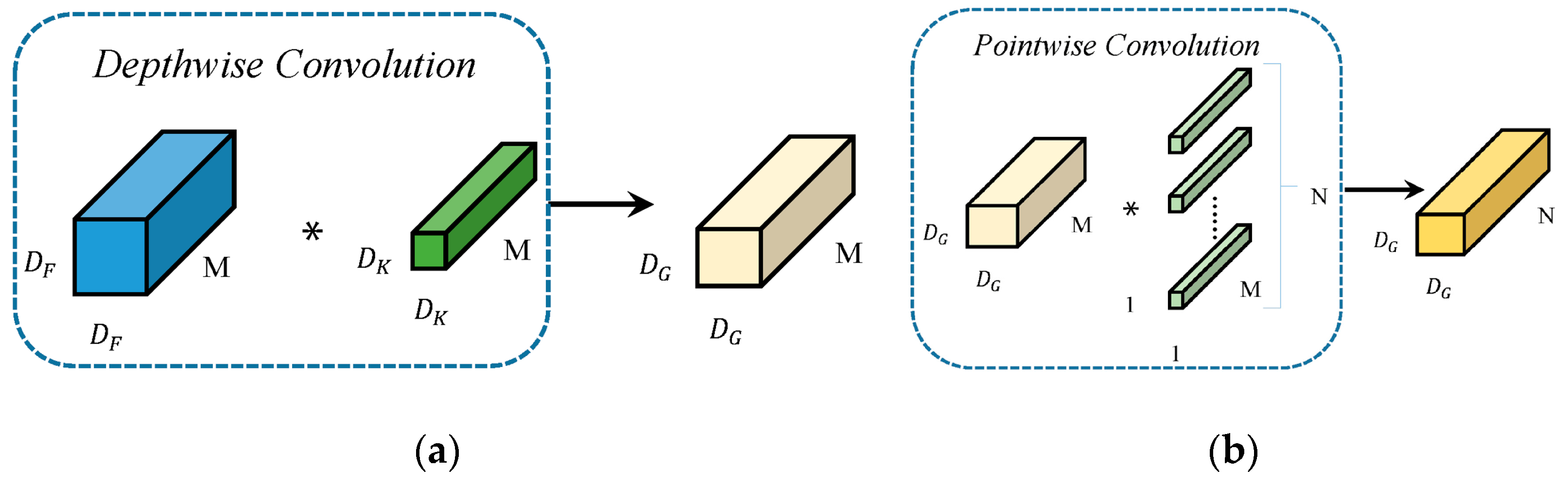
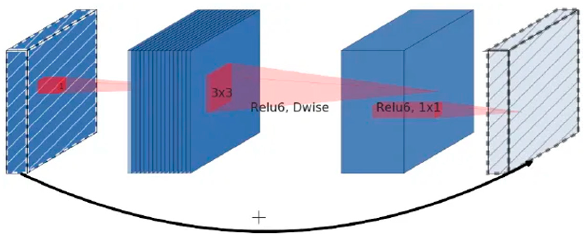
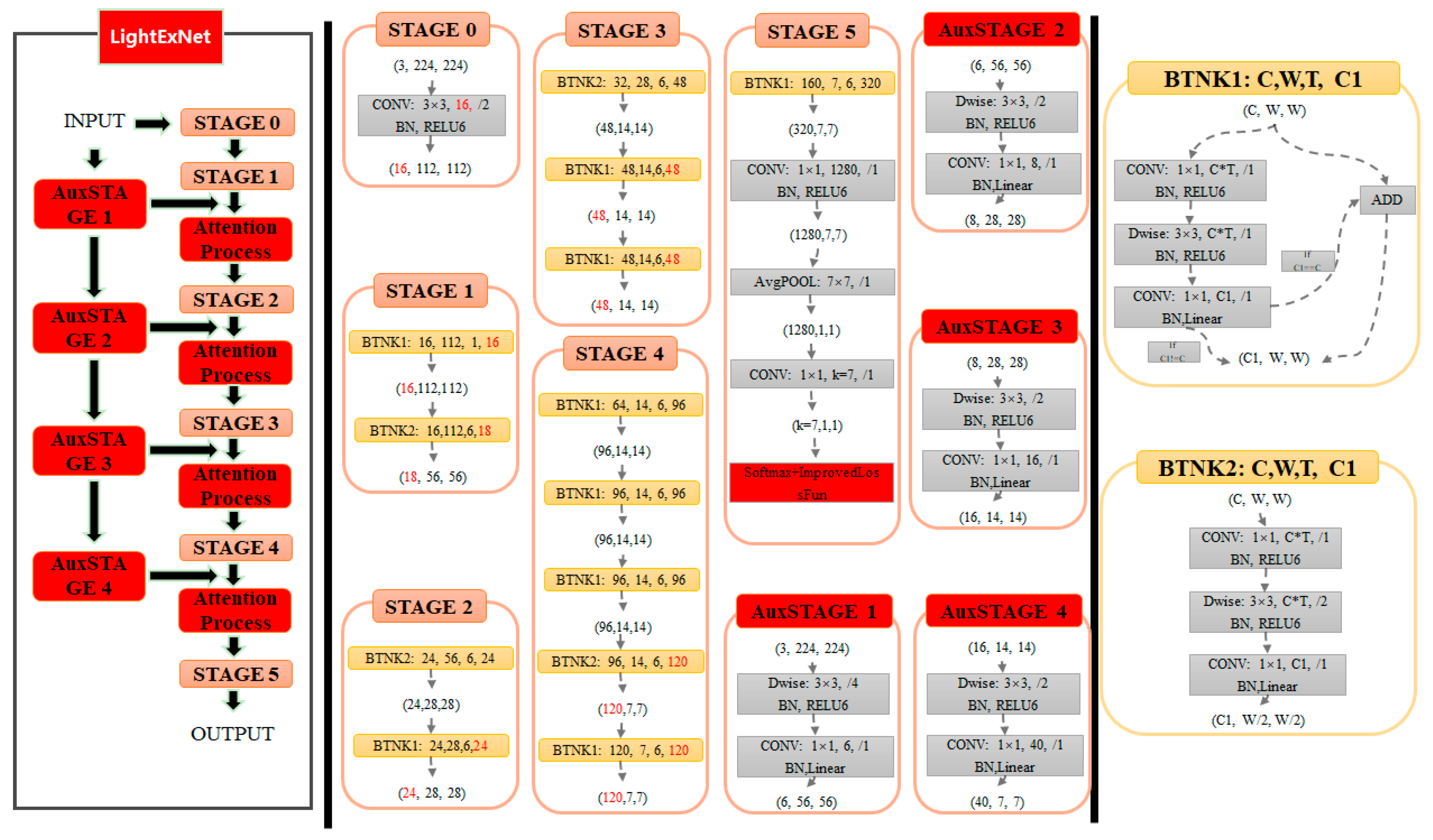
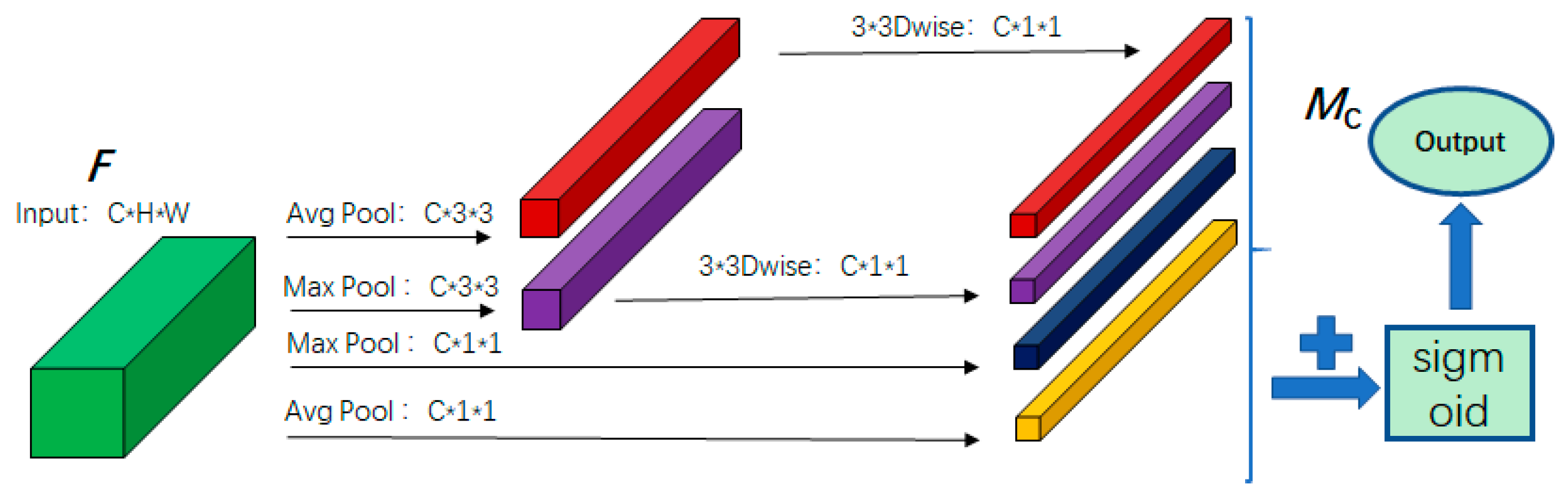
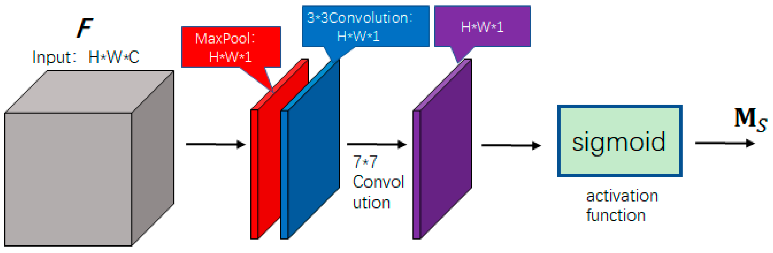
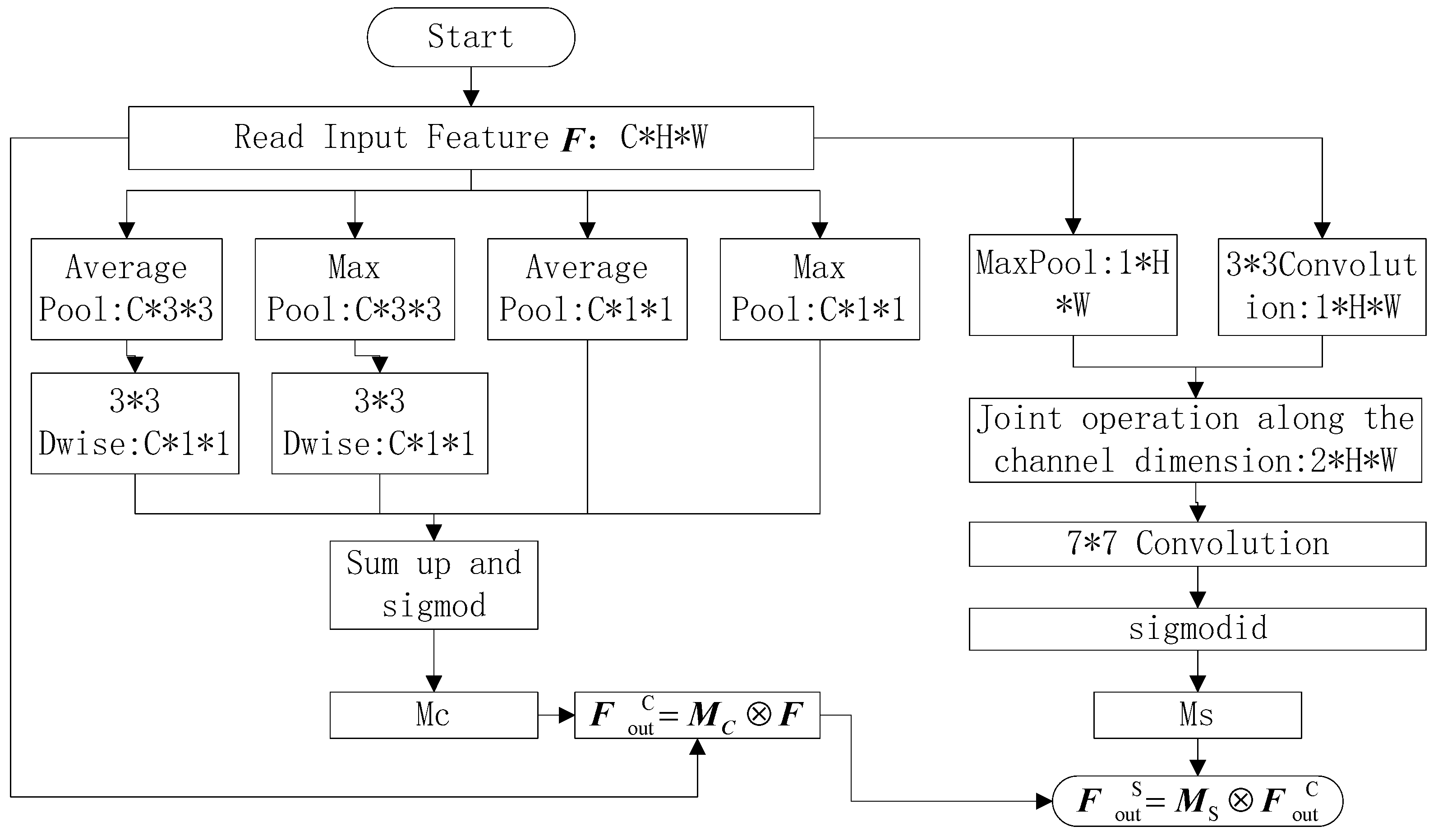
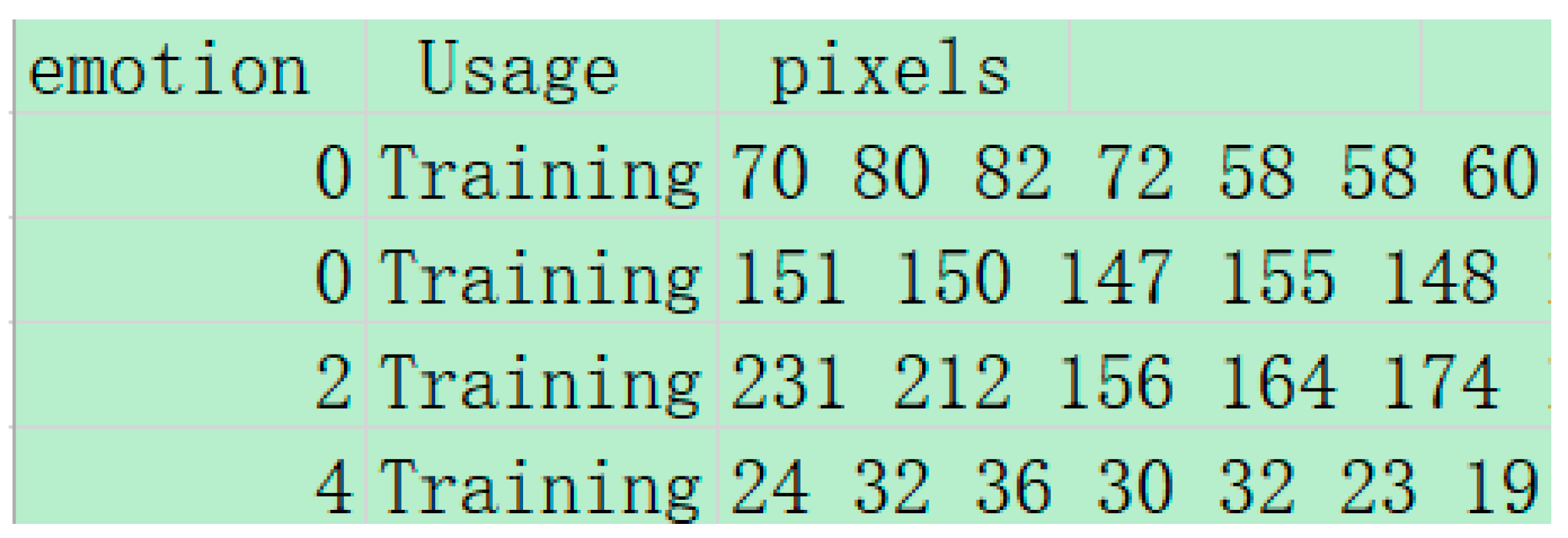
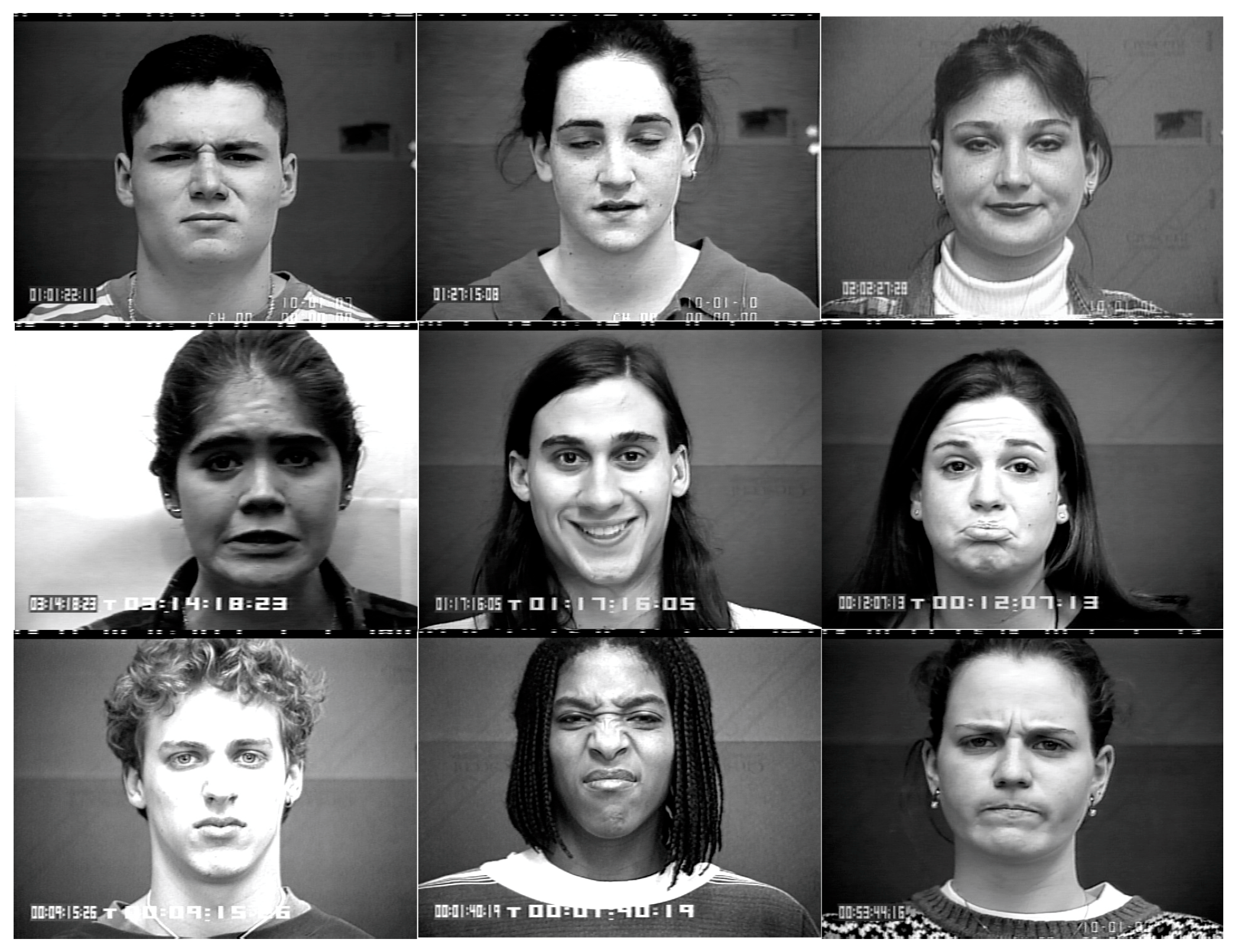

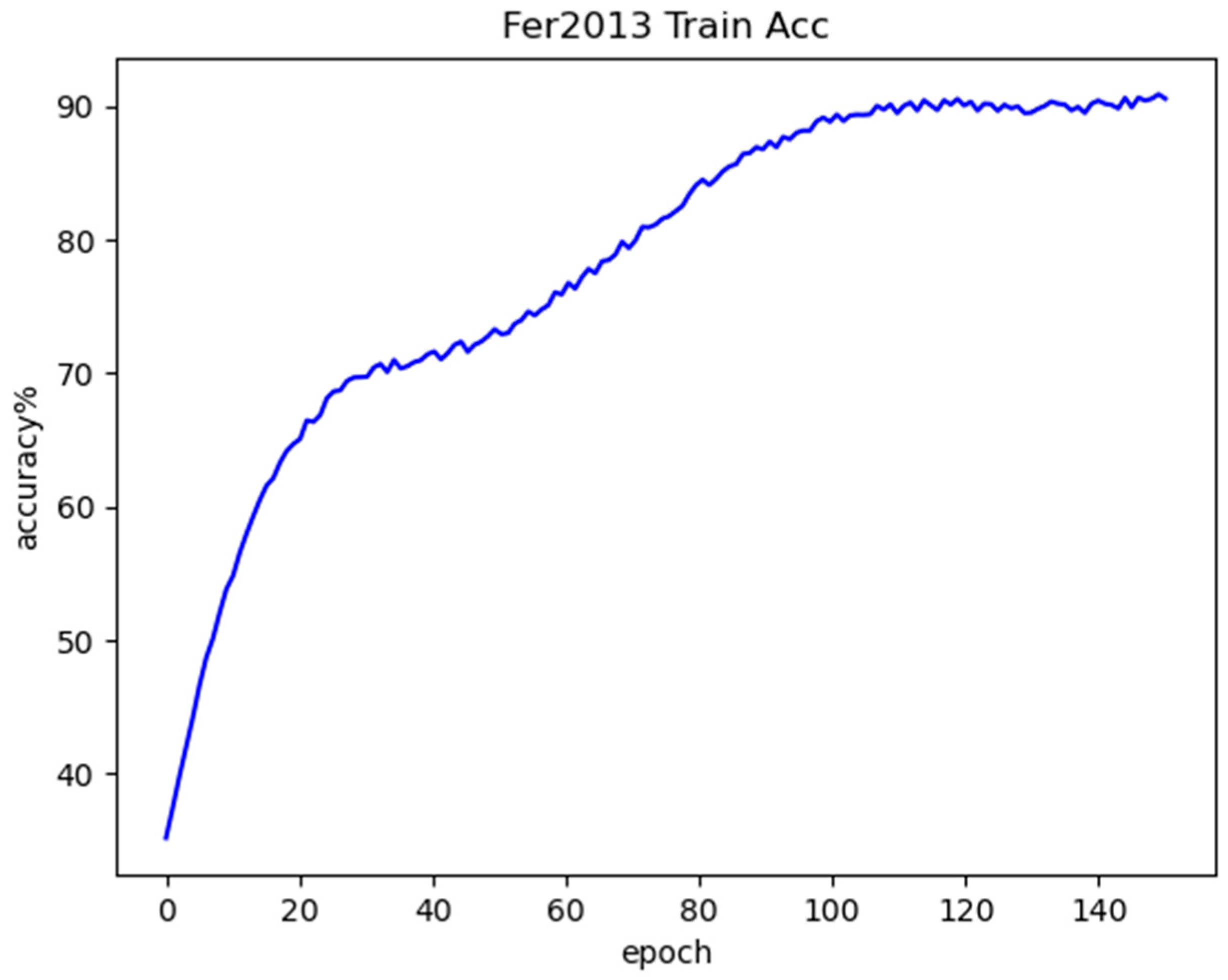
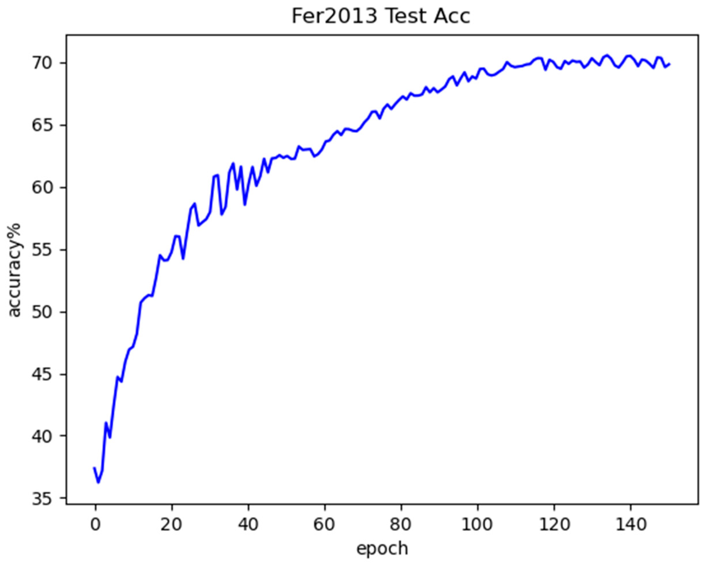
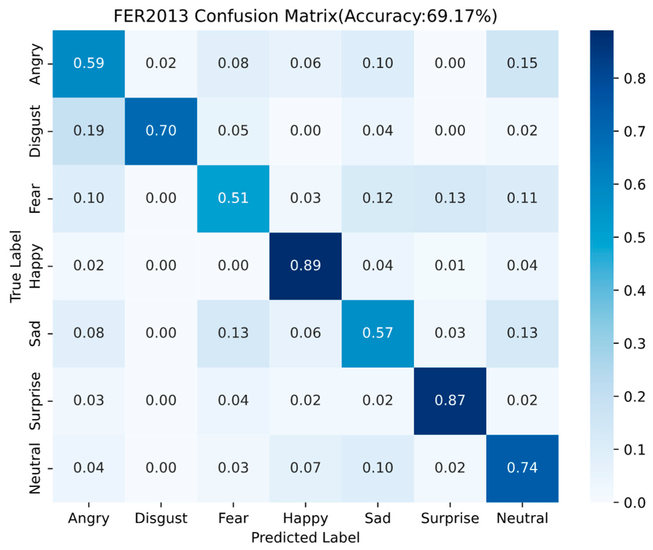
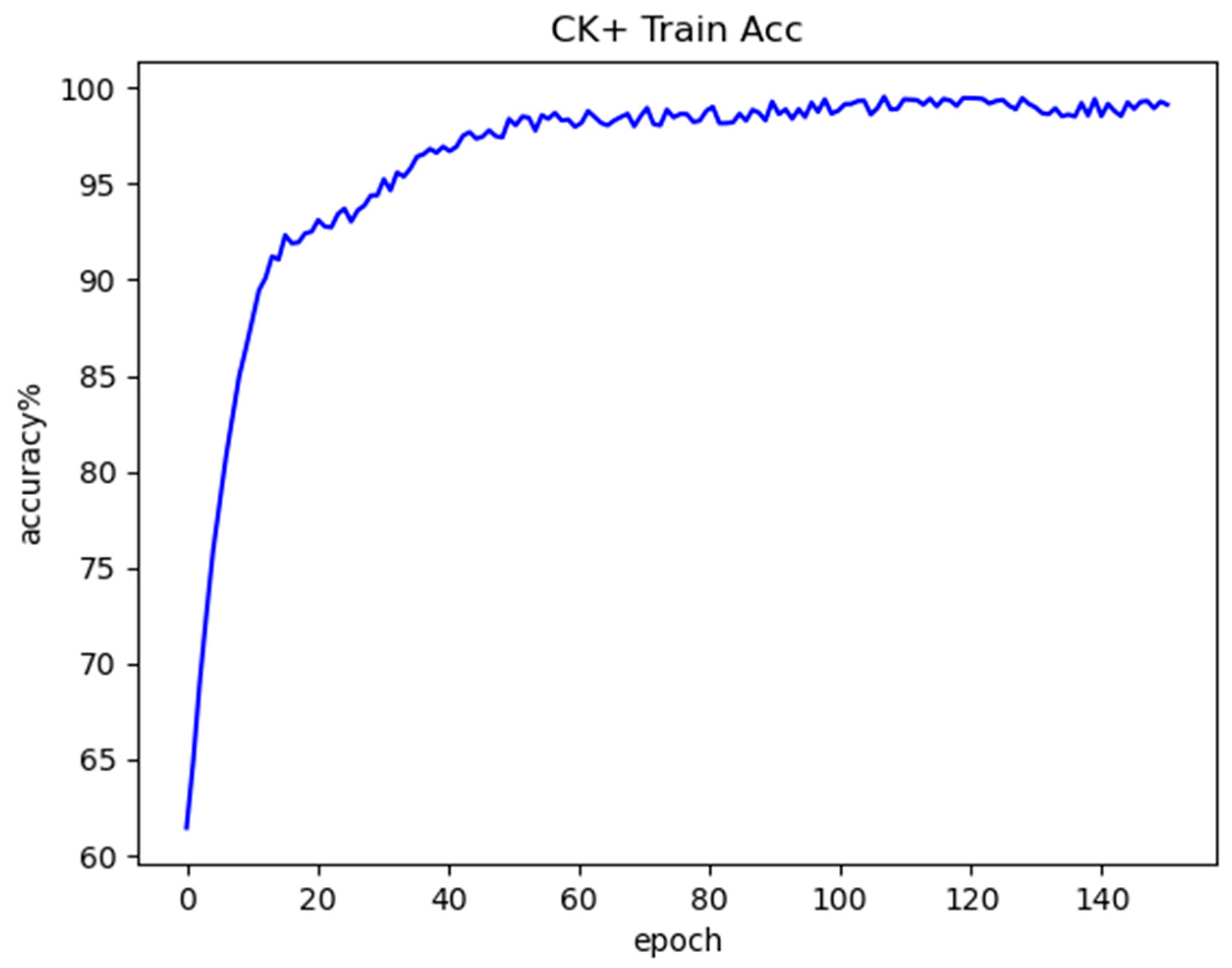
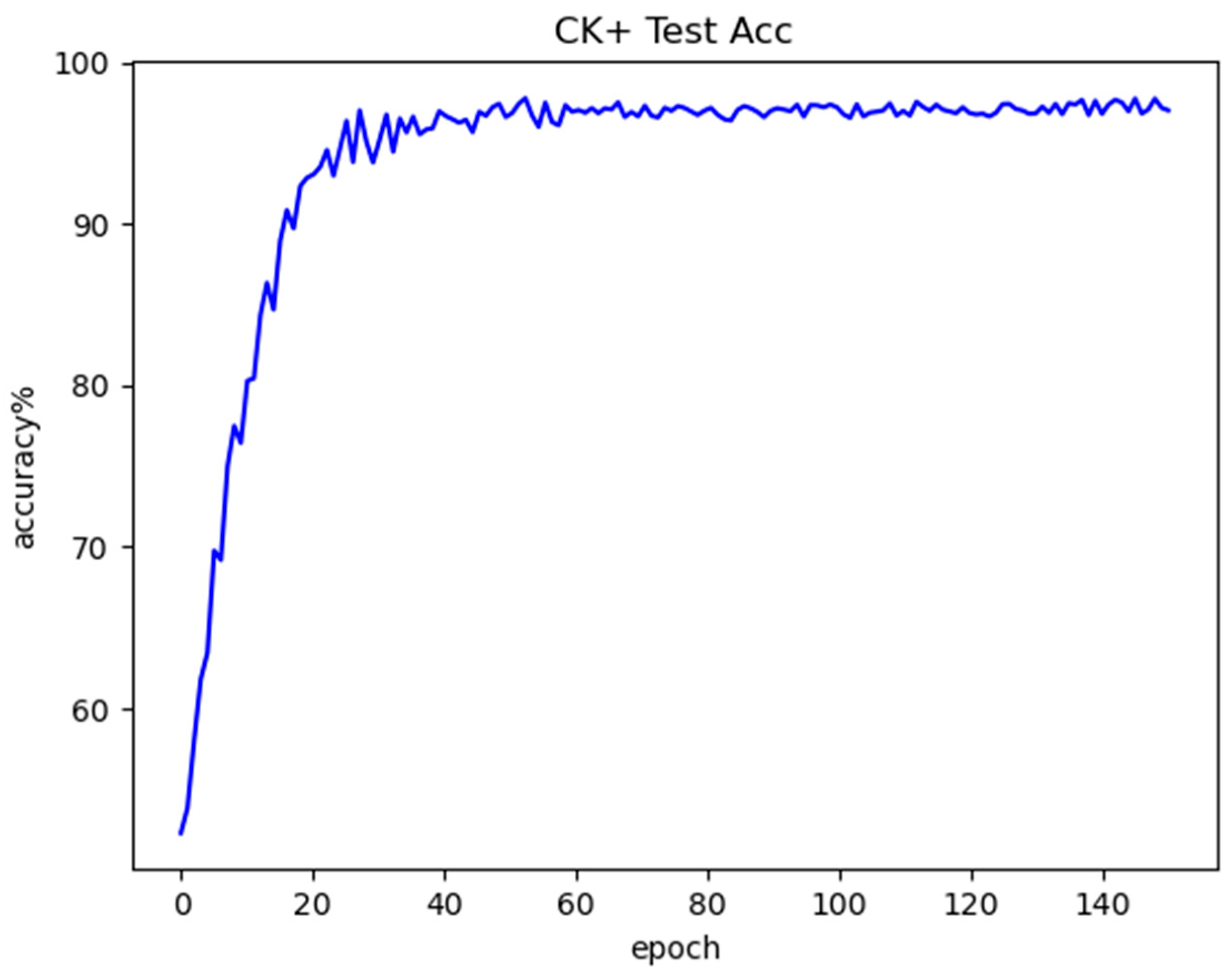
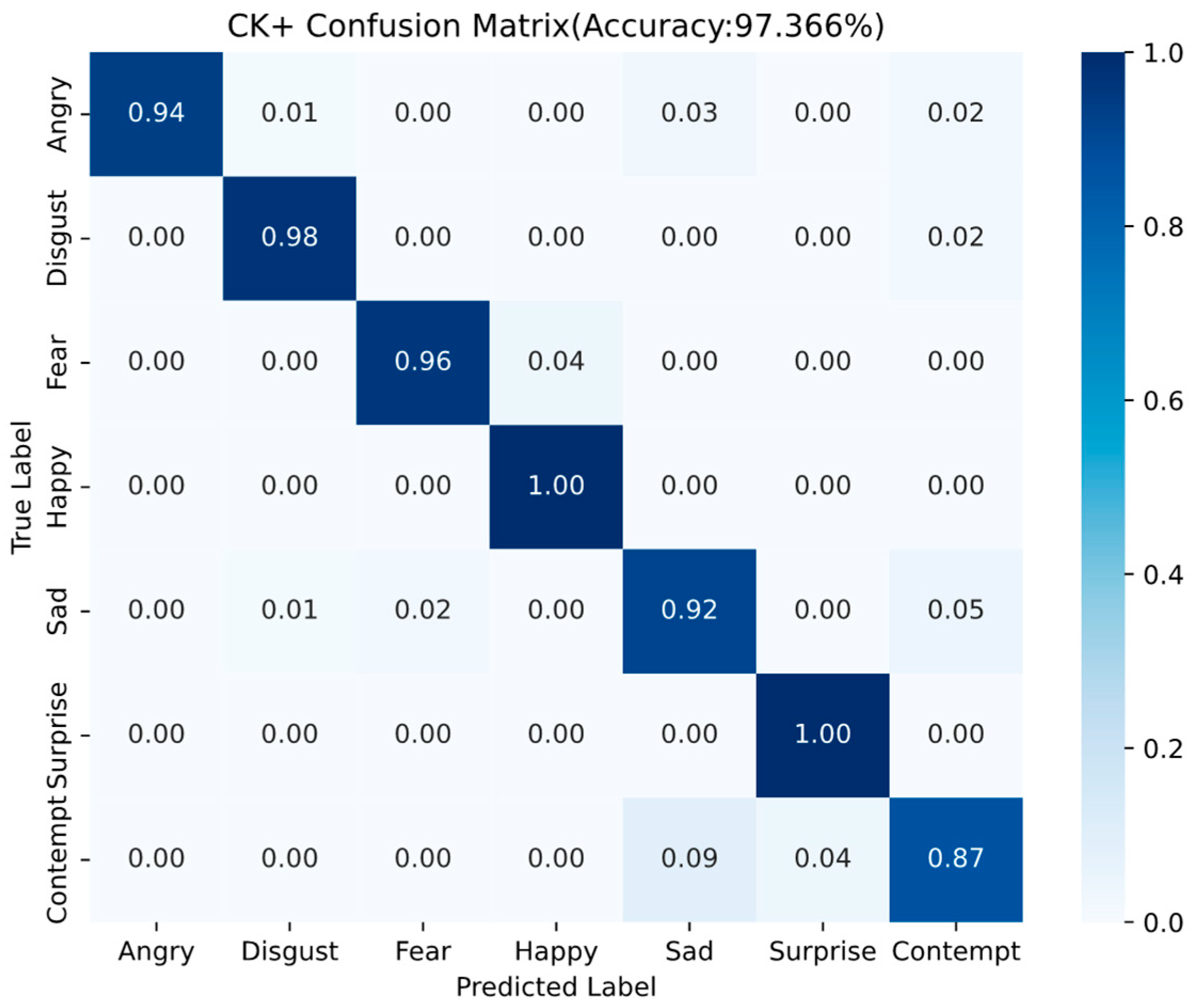
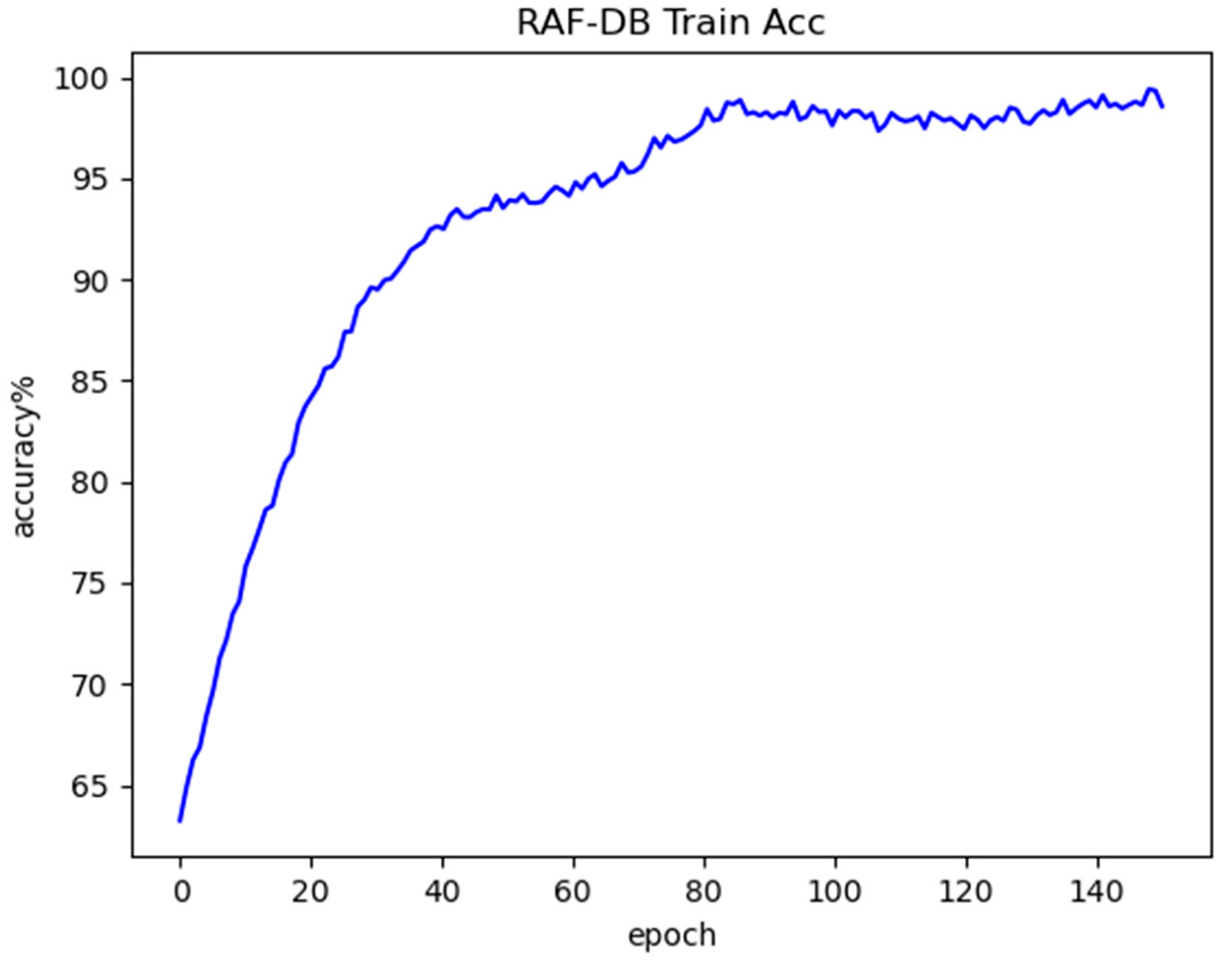
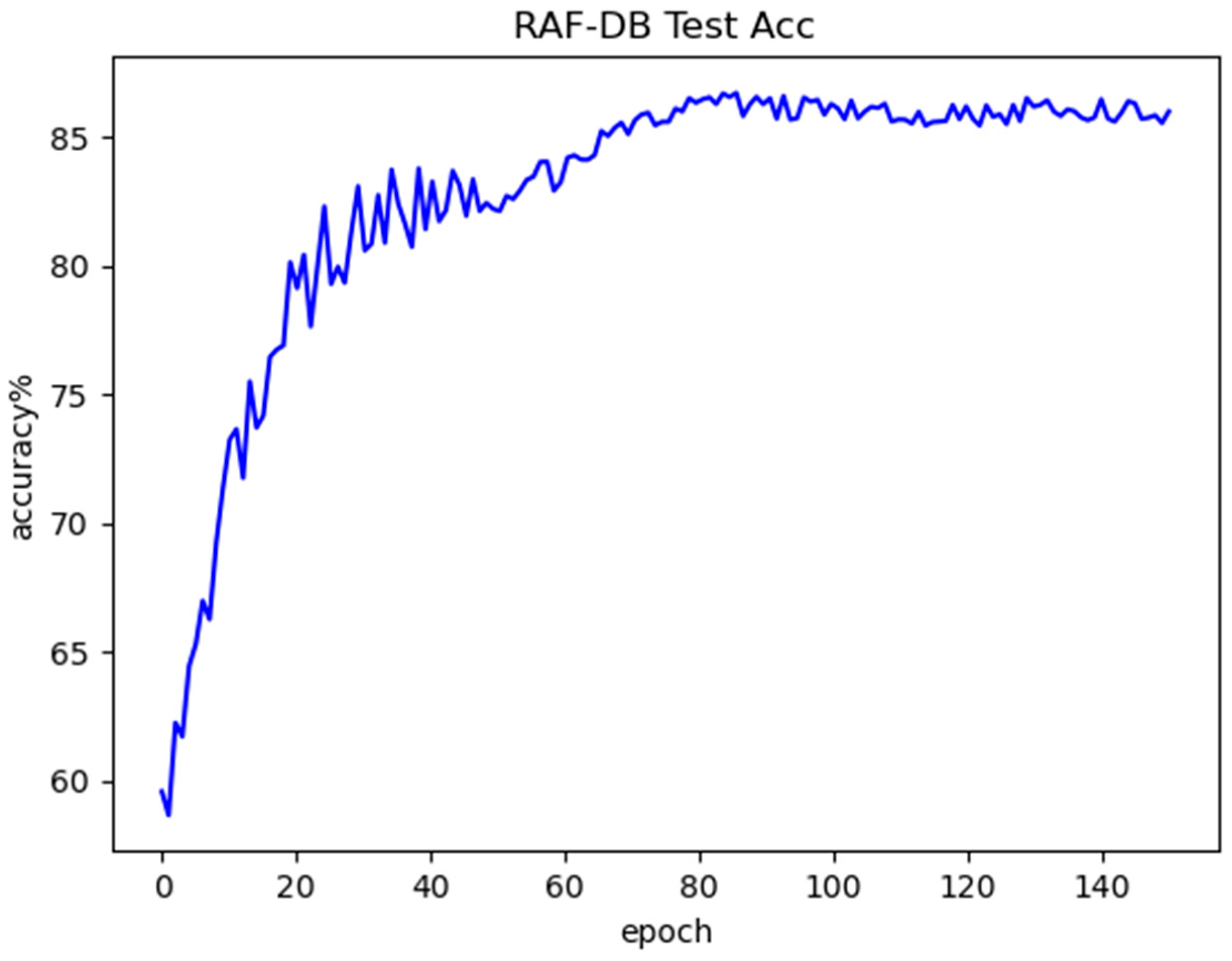
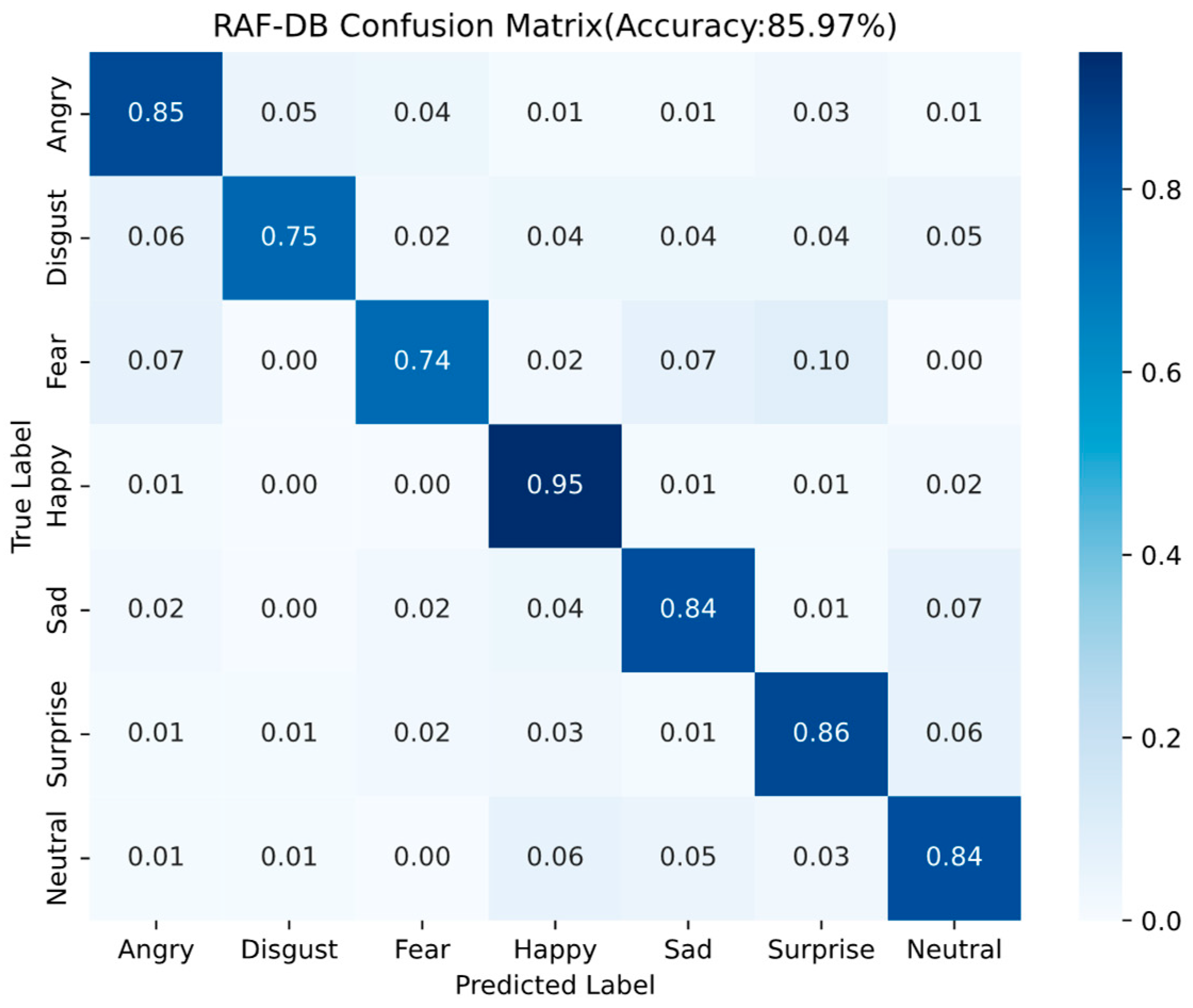
Disclaimer/Publisher’s Note: The statements, opinions and data contained in all publications are solely those of the individual author(s) and contributor(s) and not of MDPI and/or the editor(s). MDPI and/or the editor(s) disclaim responsibility for any injury to people or property resulting from any ideas, methods, instructions or products referred to in the content. |
© 2025 by the authors. Licensee MDPI, Basel, Switzerland. This article is an open access article distributed under the terms and conditions of the Creative Commons Attribution (CC BY) license (https://creativecommons.org/licenses/by/4.0/).