Feature Transformation-Based Few-Shot Class-Incremental Learning

Abstract

In the process of few-shot class-incremental learning, the limited number of samples for newly introduced classes makes it difficult to adequately adapt model parameters, resulting in poor feature representations for these classes. To address this issue, this paper proposes a feature transformation method that mitigates feature degradation in few-shot incremental learning. The transformed features better align with the ideal feature distribution required by an optimal classifier, thereby alleviating performance decline during incremental updates. Before classification, the method learns a well-conditioned linear mapping from the available base classes. After classification, both class prototypes and query samples are projected into the transformed feature space to improve the overall feature distribution. Experimental results on three benchmark datasets demonstrate that the proposed method achieves strong performance: it reduces performance degradation to 24.85 percentage points on miniImageNet, 24.45 on CIFAR100, and 24.14 on CUB, consistently outperforming traditional methods such as iCaRL (44.13–50.71 points degradation) and recent techniques like FeTrIL and PL-FSCIL. Further analysis shows that the transformed features bring class prototypes significantly closer to the theoretically optimal equiangular configuration described by neural collapse, highlighting the effectiveness of the proposed approach.

1. Introduction

Incremental learning refers to methods capable of continuously processing streams of information from the real world, while not only acquiring new knowledge but also retaining, integrating, and potentially optimizing previously learned knowledge [1]. Class-incremental learning is a form of incremental learning that aims to train a unified classifier capable of recognizing newly encountered classes over time [2]. To mitigate the problem of forgetting previously learned knowledge, class-incremental learning commonly employs knowledge distillation techniques, often supported by a small memory buffer that stores exemplars from past classes to guide the loss function during training [3]. The general form of the loss function is as follows [3]:

$$l(D^t,P;\theta )=l_{CE}(D^t,P;\theta )+\nu l_{DL}\left(\sum _{i=1}^{t-1}{D}^i,P;\theta \right),$$

(1)

where $l_{DL}$ denotes the loss term for knowledge distillation, and $l_{CE}$ represents the cross-entropy loss for the classifier. The variable t indicates the current training iteration or generation, P refers to the set of exemplars sampled from the known class set $D_i$, and $\theta$ denotes the parameters of the neural network. The implementation of the distillation term $l_{DL}$ varies across different studies.

Rebuffi et al. [4] proposed iCaRL, a pioneering method for incremental learning that addresses the problem of catastrophic forgetting in neural networks. iCaRL uses a nearest-mean-of-exemplars classifier, a K-Nearest Neighbors (KNN)-inspired approach that assigns test samples to the closest class mean in feature space, enabling efficient classification. Combined with a strategy for selecting and storing representative exemplars, iCaRL allows models to learn new classes over time while retaining performance on previously learned ones, without requiring access to all past data. Castro et al. [3] introduced an end-to-end incremental learning approach that jointly optimizes classification and distillation losses to mitigate catastrophic forgetting. Unlike methods that decouple feature learning from classification, their framework updates the entire model in an end-to-end manner, allowing the representation and classifier to evolve together as new classes are introduced. This design enables more flexible and adaptive class-incremental learning over time. Hou et al. [5] and Wu et al. [6] both addressed the prediction bias issue that arises in class-incremental learning, where the classifier tends to favor newly introduced classes due to the class imbalance between current task data and limited exemplars from past tasks. Hou et al. [5] proposed a rebalancing strategy that modifies the output layer by replacing the standard dot product with cosine similarity, which reduces the bias towards new classes by normalizing feature magnitudes. In contrast, Wu et al. [6] introduced a bias correction model that post-processes the output logits, learning a set of bias parameters from a held-out validation set to calibrate predictions. These approaches reflect two complementary perspectives: architectural adjustment at the classifier level and output-level calibration via post hoc correction, both aiming to achieve a more balanced and unified classifier in incremental settings.

Traditional class-incremental learning methods are not well-suited for few-shot scenarios. There are two main challenges [7,8]: first is the imbalance between new and old classes, where conventional strategies typically require a large amount of data to mitigate this issue—an assumption that does not hold in few-shot settings where data is scarce; second, balancing the distillation loss and the classification loss becomes more difficult, which often leads to suboptimal performance. To address incremental learning under few-shot conditions, researchers have proposed new methods tailored to these constraints. Tao et al. [9] abandoned the use of distillation loss and introduced a topology-preserving network based on the Neural Gas algorithm. Their method maintains the relative topological structure among class prototypes, enabling the model to retain old knowledge while adapting to new classes in a few-shot incremental setting. In contrast, Zhang et al. [10] proposed a decoupled approach where the feature extractor remains fixed and only the classifier is continually updated. They employed a graph attention network to capture semantic relationships between old and new class prototypes, resulting in an evolving KNN-based classifier that effectively balances stability and plasticity throughout the incremental learning process. Recent modular and attention-based designs have also shown promise in improving representation robustness in multi-domain settings. For instance, Chechkin et al. [11] proposed a hybrid KAN-BiLSTM Transformer, which leverages dynamic attention and architectural modularity to effectively process structurally diverse inputs. These strategies offer valuable insights for FSCIL under few-shot constraints, where feature distribution alignment is critical yet data is limited. Lightweight adaptation techniques such as LoRA [12] and Adapters [13] have been proposed to efficiently fine-tune large pre-trained models by injecting small trainable modules into frozen backbones. These methods have demonstrated strong performance in few-shot and incremental learning scenarios, highlighting the potential benefits of low-rank or bottleneck-based parameter adaptation.

However, these methods still struggle to avoid the phenomenon of neural collapse in few-shot class-incremental learning [14]. Neural collapse refers to a special convergence behavior and feature space degeneration observed when training neural networks with a limited number of samples in an incremental setting. Specifically, the weights of the final classification layer are disrupted by the newly added data, rendering the original classifier ineffective. This phenomenon highlights that a well-performing classifier requires its final-layer weights to be aligned with the class prototypes, and that the class centers should be as well-separated as possible [15]. Mathematically, the neural collapse phenomenon is characterized by several distinct properties: (1) classifier weights and class means become aligned, forming a simplex equiangular tight frame (ETF) where the angle (or cosine similarity) between any pair of class prototypes is equal; (2) within-class variability collapses, meaning features from the same class concentrate around the class mean; and (3) all class prototypes lie on a sphere and are maximally separated in angular space. These characteristics can be quantitatively assessed via pairwise inner products or angular deviations between normalized class means.

A common strategy to mitigate this issue is feature transformation, which aims to map features from the current space to a more desirable feature space where the effects of neural collapse are minimized. Traditionally, feature transformation is a technique used in transfer learning to reduce distributional shifts between the source and target domains [16]. Based on whether the distance metric is explicitly defined, feature transformation methods can be categorized into statistical and geometric approaches [17]. Statistical feature transformation explicitly specifies a distance measure, whereas geometric methods rely on an implicit metric derived from the geometric properties of the data. The core idea of both approaches is to minimize the distributional discrepancy between the source and target domains under a certain metric. For statistical methods, one of the most widely used metrics is Maximum Mean Discrepancy (MMD). For example, Transfer Component Analysis (TCA) [18] assumes that the conditional distributions across domains are identical, while the marginal distributions differ. By minimizing the MMD between the source and target domain marginals, TCA aligns the joint distributions of the two domains. In contrast, geometric transformation methods do not explicitly measure distributional differences but instead reduce domain shift by leveraging geometric structure in the data through appropriate transformations. For example, the subspace alignment method [19] learns a linear transformation that aligns the geometric structure of the source domain with that of the target domain, thereby reducing domain differences through subspace matching.

Traditional feature transformation methods in transfer learning typically require access to both source and target domain data. Recent advances in feature transformation for exemplar-free and few-shot class-incremental learning include FeTrIL [20], which explicitly performs geometric translation of new class features to generate pseudo-features of past classes for stable incremental learning, and PL-FSCIL [21], which implicitly transforms features by integrating domain-specific and task-specific prompts into the attention layers of pre-trained Vision Transformers to enhance adaptability to new classes with few samples.

In the scenario considered in this work, the target domain, which is defined as the ideal feature distribution aligned with the condition of neural collapse, is not directly available. To address this, we propose a learnable linear transformation module. Under a fixed feature extractor, we sample various few-shot tasks from a base dataset to train the transformation module to improve classification performance. During incremental learning, data from each stage is processed sequentially through the frozen feature extractor and the learned transformation module to produce final representations.

2. Problem

The goal of few-shot class-incremental learning is to incrementally train a model on a sequence of training datasets $\{D^{\left(0\right)},D^{\left(1\right)},\dots ,D^{\left(T\right)}\}$, where $D^{\left(0\right)}$ is a base dataset and T is the number of incremental learning steps. Each dataset $D^{\left(t\right)}={\left\{(x_i,y_i)\right\}}_{i=1}^{|D^{\left(t\right)}|}$ represents the data introduced at the t-th learning stage. The base dataset $D^{\left(0\right)}$ corresponds to a relatively large label space $C^{\left(0\right)}$, and for each class $c\in C^{\left(0\right)}$, a sufficient number of training samples are available. In contrast, each incremental dataset $D^{\left(t\right)}$ (for $t>0$) contains only a small number of samples, with the total number given by $|D^{\left(t\right)}|=N\times K$, where N is the number of classes and K is the number of samples per class—following the same task setup as the N-way K-shot paradigm in few-shot learning.

The label spaces of different incremental stages are mutually disjoint, i.e., $C^{\left(t\right)}\cap C^{\left(t^{\prime }\right)}=\varnothing$, for all $t^{\prime }\ne t$. During the t-th training stage ($t>0$), only the dataset $D^{\left(t\right)}$ is accessible; data from previous stages is not available. At test time for stage t, the model is evaluated on test samples drawn from all classes seen so far, i.e., the test label space is ${\cup }_{i=0}^t{C}^{\left(i\right)}$.

3. Feature Transformation

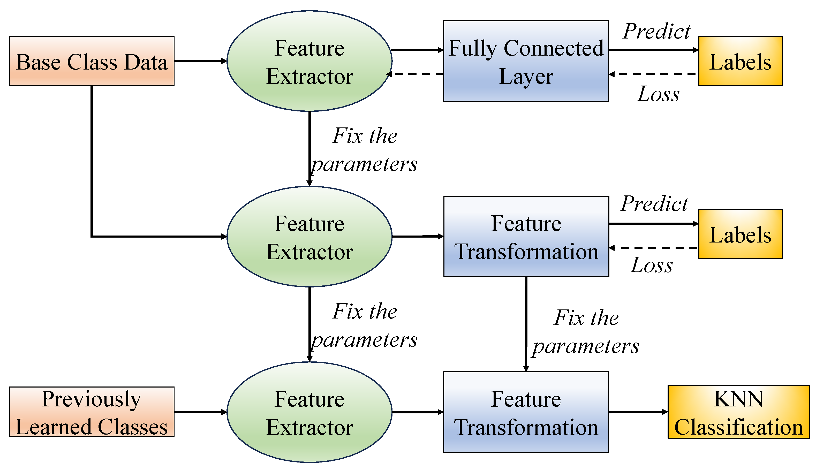
An illustration of our proposed feature transformation-based few-shot class-incremental learning framework is shown in Figure 1. First, a feature extractor is trained on the base classes. The feature extractor’s parameters are then frozen, and multiple few-shot tasks are sampled from the base dataset to train the feature transformation module until convergence. After training, classification is performed using a KNN classifier. For previously learned classes, our method maintains a class prototype (or class center) for each category. During the classification stage, each test sample is sequentially passed through the feature extractor and the feature transformation module. The resulting feature is then compared with all stored class prototypes to determine the final predicted label.

3.1. Feature Extractor

We first train a standard classification network f using the base dataset $D_B$. The base dataset is divided into a training set $D_{B_{train}}={\left\{(x_i,y_i)\right\}}_{i=1}^{b_0}$ and a test set $D_{B_{test}}={\left\{(x_j,y_j)\right\}}_{j=1}^{b_1}$, where $b_0$ and $b_1$ denote the number of samples in the training and test sets, respectively. The classification network is trained by minimizing the empirical risk:

$$arg\underset{f}{min}\sum _{(x_j,y_j)\in D_{B_{train}}}l(f\left(x_j\right),y_j)$$

(2)

where $l(·,·)$ is the loss function, typically the cross-entropy loss used in classification tasks.

The classification network consists of two parts: a feature extractor and a fully connected (FC) layer. It can be represented as

$$f\left(x\right)=W^T\varphi \left(x\right)+\mathrm{bias}$$

(3)

where $\varphi (·):{\mathbb{R}}^D\to {\mathbb{R}}^d$ denotes the feature extractor, which maps the input from the original feature space ${\mathbb{R}}^D$ to a lower-dimensional feature space ${\mathbb{R}}^d$, extracting compact and discriminative features. $W^T\in {\mathbb{R}}^{d\times |Y_B|}$ and $bias$ represent the weights and bias of the FC layer, respectively. Once the network is fully trained and converged, the FC layer is removed, and only the feature extractor $\varphi (·)$ is retained. In all subsequent stages of the proposed method, feature representations are obtained using the fixed feature extractor $\varphi (·)$.

3.2. Feature Transformation

In the scenario considered in this work, the target domain data which is defined as an ideal distribution consistent with the neural collapse phenomenon is not available. In our implementation, the feature transformation is designed to produce class prototypes that approximate the ETF structure implied by neural collapse. By encouraging equiangularity and reduced intra-class variance in the transformed space, we aim to better align the learned features with the theoretically optimal configurations. Therefore, we propose a trainable linear transformation method by introducing an additional feature transformation layer, which is trained after the feature extractor has been learned. Both the feature extractor and the transformation layer are then fixed for incremental learning and evaluation. Specifically, the feature transformation layer is implemented as a fully connected layer with its bias term set to zero, followed by an ${\ell }_2$ normalization applied to the output. The input and output dimensions are both set to 512, consistent with the dimensionality of the feature extractor output. No Dropout or Batch Normalization is applied within the transformation layer. The weight matrix is initialized using a Gaussian distribution with zero mean and variance $1/d$, where $d=512$.

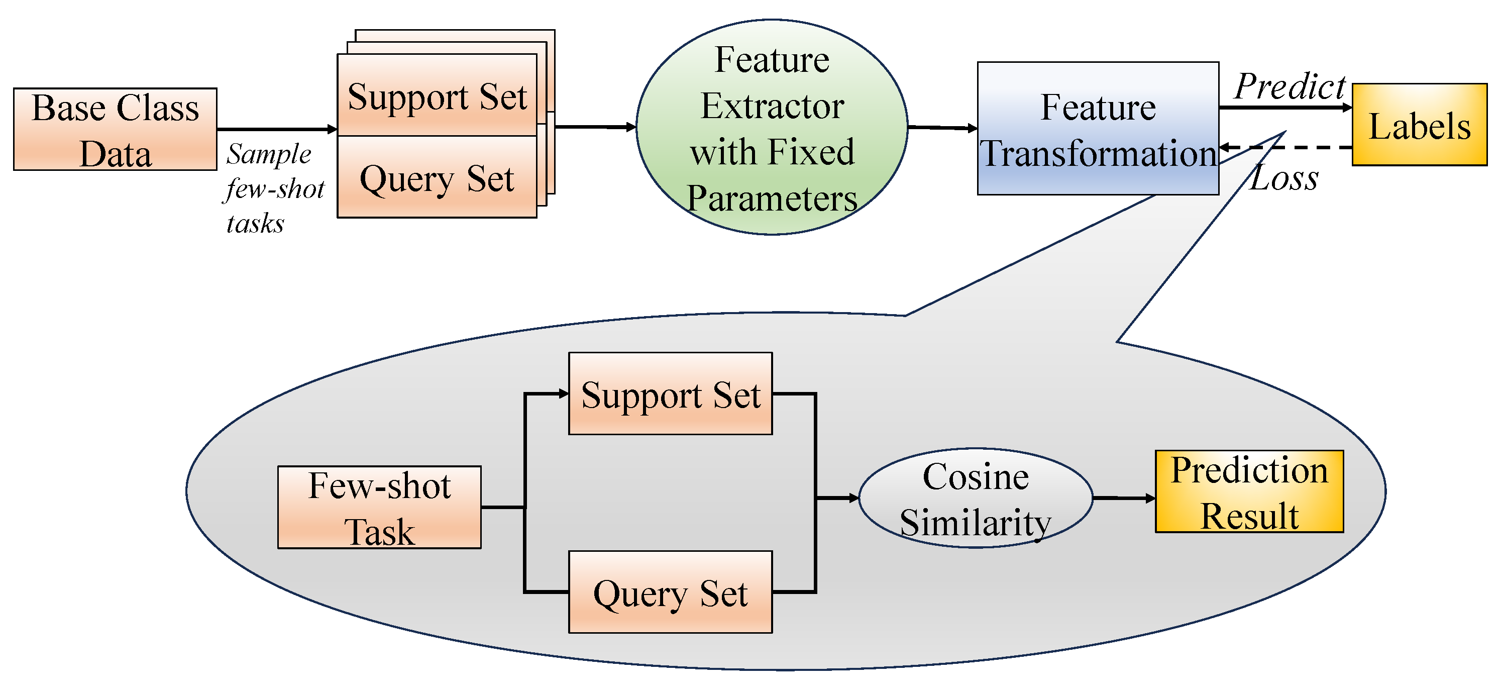
The training process for the feature transformation layer is illustrated in Figure 2. The layer is initialized using a Gaussian distribution with zero mean and a variance equal to the reciprocal of the feature dimension. A series of few-shot tasks, each consisting of a support set and a query set, are sampled from the base classes. All samples are first passed through the feature extractor and then through the transformation layer. The transformed query samples are classified using cosine similarity with the transformed support samples. Since the support set is labeled, predictions for the query set can be made based on the similarity scores. Cross-entropy loss is used to supervise the predictions, and the parameters of the transformation layer are updated via gradient descent. Each sampled few-shot task follows a 15-way 1-shot setting, with 15 query samples per class used to construct the query set.

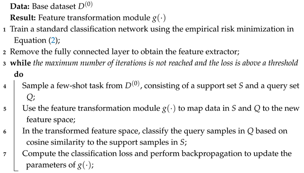
The training process of the proposed feature transformation method is shown in Algorithm 1.

Algorithm 1: Training procedure of the feature transformation module using the base dataset

The computational cost of Algorithm 1 is dominated by two parts: (1) feature extraction using the fixed backbone network (e.g., ResNet), and (2) the linear transformation module. In each iteration, the complexity of extracting features for the support and query samples is $O((N_S+N_Q)·C)$, where C denotes the computational cost per sample of the convolutional backbone, and $N_S$ and $N_Q$ are the numbers of support and query samples, respectively. The linear transformation, implemented as a 512 × 512 fully connected layer, adds $O((N_S+N_Q)·{512}^2)$ operations per iteration. Computing cosine similarities between every query–support pair requires $O(N_Q·N_S·d)$ operations. Overall, for T iterations, the total training complexity is $O(T·((N_S+N_Q)·(C+{512}^2)+N_Q{N}_{S}d))$. In high-dimensional feature spaces (e.g., 512 dimensions), the training complexity remains controlled because the cost of the linear transformation is negligible compared to the convolutional backbone. During inference, the additional cost introduced by the transformation layer is minimal, involving only a single 512 × 512 matrix multiplication and normalization per sample. Combined with cosine similarity calculations with stored class prototypes, this results in very efficient inference without significant overhead compared to standard fixed-feature extractor methods.

3.3. Classification

After feature transformation, the proposed method performs final classification using the KNN approach. A set of class prototypes is maintained to support the classification process. For base classes, features of all training samples are extracted using the best-performing feature extractor obtained during training, and the mean feature vector of each class is computed and stored as its class prototype. For incremental classes, the prototype is calculated as the mean of the features extracted from the support set samples. During inference, the test sample and all class prototypes are passed through the same feature transformation module. Classification is then performed based on cosine similarity: the test sample is assigned to the class whose prototype has the highest cosine similarity with the test feature.

4. Simulation Experiments

The simulations consist of two parts: baseline and ablation experiments. The baseline experiments evaluate the proposed method on few-shot class-incremental learning tasks across three benchmark datasets. The ablation experiments analyze the difference between the feature distributions before and after transformation compared to the theoretical optimal distribution, as well as the impact of relevant hyperparameters on the model’s performance. Additionally, the ablation section includes performance comparisons between the proposed method and other commonly used feature transformation techniques.

4.1. Experimental Setup

We evaluate our method on three widely used benchmark datasets in few-shot class-incremental learning: CIFAR100 [22], miniImageNet [23], and CUB [24]. CIFAR100 contains 100 classes. Following the split protocol in [9], we use 60 classes as base classes and the remaining 40 as novel classes. The novel classes are introduced over 8 incremental sessions, with 5 new classes added per session. The miniImageNet also contains 100 classes. We follow the same partitioning strategy as in [9], using 60 classes as base classes and 40 classes as novel ones. The 40 novel classes are divided into 8 incremental sessions, each adding 5 new classes. CUB contains 200 classes. Following [9], we use 100 classes as base classes and the other 100 as novel classes. These 100 novel classes are divided into 10 incremental sessions, each introducing 10 new classes.

To ensure fair comparison, we use ResNet-20 as the feature extractor for CIFAR100, and ResNet-18 for miniImageNet and CUB. Both feature extractors include Batch Normalization after each convolutional block and apply Dropout with a rate of 0.5 before the final fully connected layer. The optimizer is Stochastic Gradient Descent (SGD) with a learning rate of 0.1 and momentum of 0.9. The learning rate decays by 0.0005 every 20 epochs, and the total number of training epochs is 100. Cross-entropy loss is used, and the batch size is set to 128. In each incremental session, a 5-shot setting is used, meaning that only 5 labeled samples per new class are available for training. During evaluation, we sample 100 test instances per class from all classes learned so far, and use them to assess the performance of the model after each incremental step.

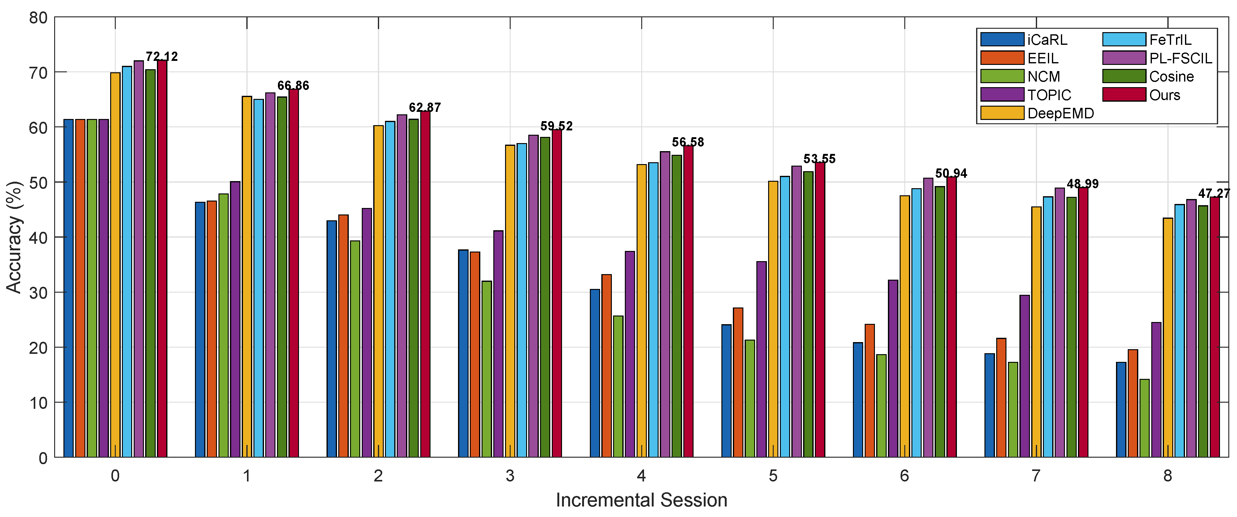
4.2. Baseline Experiments

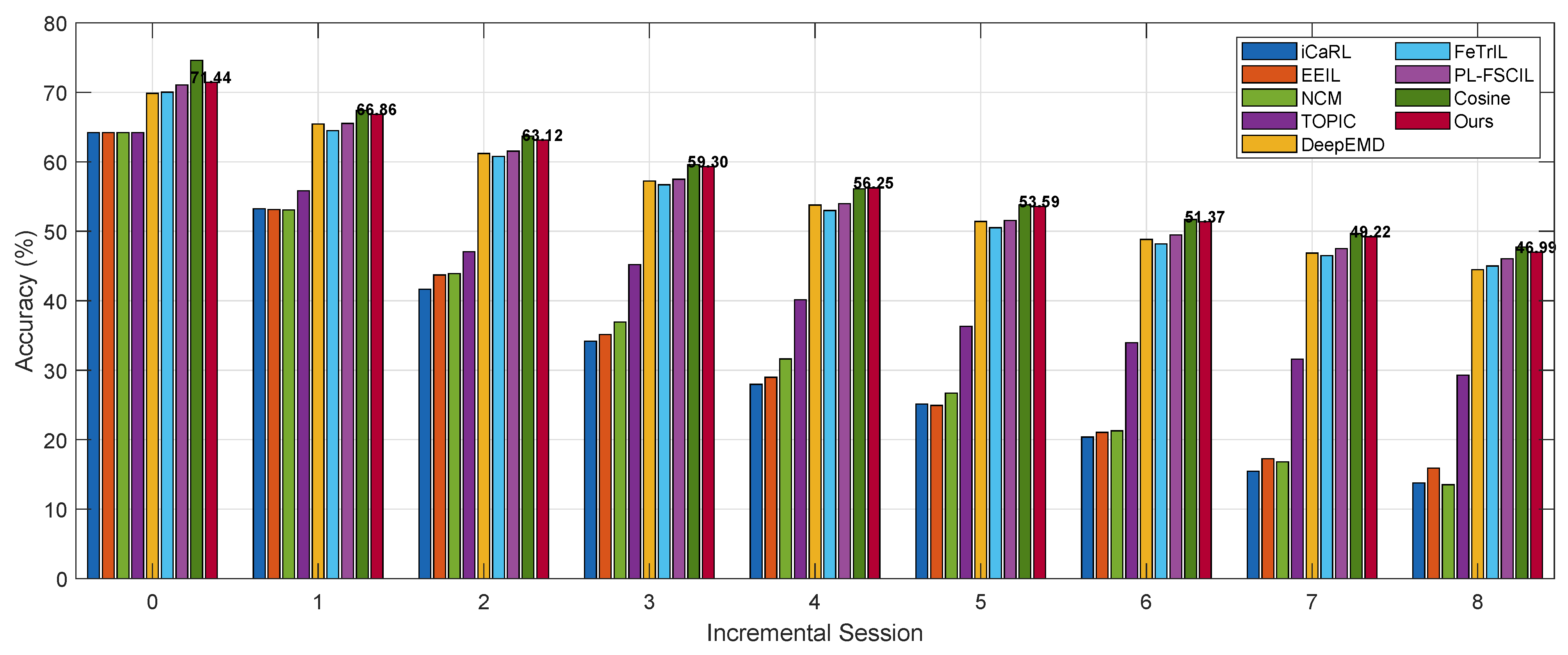
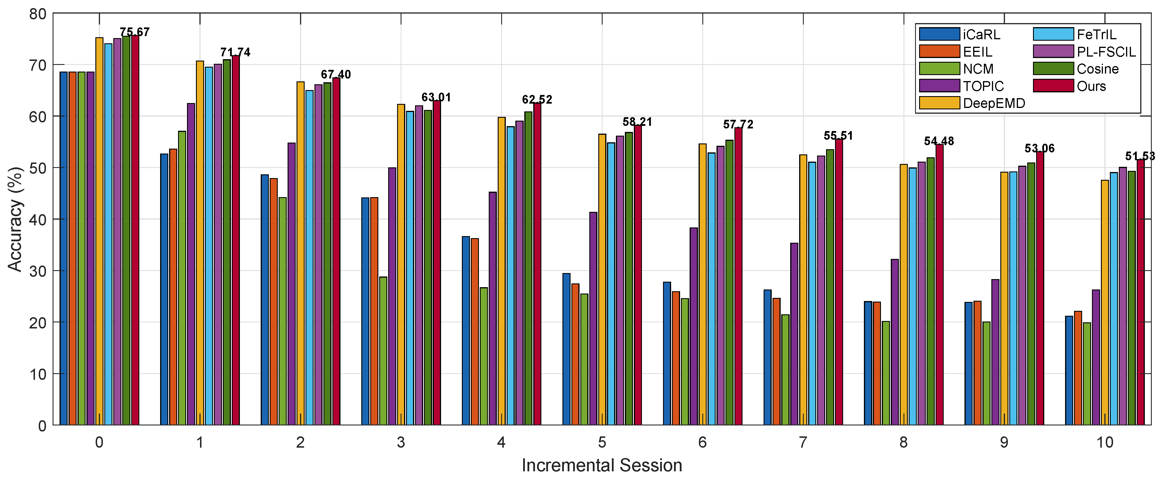
The classification results on the three datasets are reported in Figure 3, Figure 4 and Figure 5, and

Table 1. Performance degradation comparison on miniImageNet.

Method	Performance Degradation	Method	Performance Degradation
iCaRL [4]	44.13	FeTrIL [20]	26.13
EEIL [3]	41.82	PL-FSCIL [21]	25.07
NCM [5]	47.21	Cosine	24.74
TOPIC [9]	36.89	Ours	24.85
DeepEMD [25]	26.41

,

Table 2. Performance degradation comparison on CIFAR100.

Method	Performance Degradation	Method	Performance Degradation
iCaRL [4]	50.45	FeTrIL [20]	25.02
EEIL [3]	48.33	PL-FSCIL [21]	24.94
NCM [5]	50.71	Cosine	26.87
TOPIC [9]	34.92	Ours	24.45
DeepEMD [25]	25.40

and

Table 3. Performance degradation comparison on CUB.

Method	Performance Degradation	Method	Performance Degradation
iCaRL	47.41	FeTrIL	26.37
EEIL	46.49	PL-FSCIL	25.33
NCM	48.72	Cosine	26.22
TOPIC	42.33	Ours	24.14
DeepEMD	27.70

, respectively. Performance degradation is a metric proposed in [10], defined as the difference between the classification accuracy in the first session and that in the final session during the incremental learning process.

Among the compared methods, iCaRL [4], EEIL [3], and NCM [5] are traditional class-incremental learning approaches, which have been adapted in this work for the few-shot class-incremental learning (FSCIL) setting. TOPIC [9] is a method specifically designed for FSCIL. All four of these methods adopt a non-fixed feature extractor strategy, meaning the feature extractor can be fine-tuned using the new class data during the incremental process. In contrast, DeepEMD [25], FeTrIL [20], PL-FSCIL [21], Cosine, and our proposed method adopt a fixed feature extractor strategy. That is, a feature extractor is trained first to project samples into a high-dimensional feature space, and all downstream classification methods operate on these extracted features. DeepEMD is a few-shot classification method that uses Earth Mover’s Distance (EMD) for classification. Cosine performs classification directly based on cosine similarity. FeTrIL uses a fixed feature extractor and generates pseudo-features by translating new class features, enabling exemplar-free incremental learning with a simple linear classifier. PL-FSCIL builds on a pre-trained Vision Transformer with fixed features, adding Domain and FSCIL prompts to improve adaptation and incremental learning, while a prototype classifier preserves performance on old and new classes.

Our proposed method achieves strong performance on both the miniImageNet and CUB datasets. It not only obtains the highest accuracy across all incremental sessions but also exhibits the lowest performance degradation. On miniImageNet and CUB, the performance results are decreased by 24.85 and 24.14 percentage points, respectively. On the CIFAR100 dataset, while our method ranks second in per-session accuracy—slightly lower than Cosine—it still achieves the lowest performance degradation, at 24.45 percentage points. Our approach can be viewed as an enhancement to the Cosine method by introducing a feature transformation layer. This layer maps both the support and query samples of few-shot tasks into a new space, refining the estimation of class prototypes and thus improving overall performance. Although our method performs slightly worse than Cosine on CIFAR100, it outperforms all baselines on the other two datasets. Upon further analysis, we attribute this observation to differences in the dataset characteristics and distribution. While our method may have some limitations in terms of robustness, it achieves the best overall performance across all three benchmarks.

In addition, several other observations can be drawn from the figures and tables:

Compared to traditional class-incremental learning methods directly applied to few-shot settings, methods specifically designed for few-shot class-incremental learning achieve significantly better performance. For example, TOPIC, DeepEMD, FeTrIL, PL-FSCIL, and Cosine consistently outperform iCaRL, EEIL, and NCM in terms of both per-session accuracy and overall performance degradation. This highlights a fundamental shift in the nature of the problem under the few-shot constraint: the limited number of samples for new classes increases the risk of overfitting during the incremental process, which in turn degrades model performance.

Moreover, methods that keep the feature extractor fixed clearly outperform those that fine-tune the feature extractor during incremental learning. For instance, on the miniImageNet dataset, methods with a fixed feature extractor exhibit an average performance degradation of 25.44 percentage points, while those that fine-tune show a significantly higher average degradation of 42.51 percentage points. Our analysis suggests that this is due to the insufficient number of new class samples, which makes fine-tuning the feature extractor less effective. Whether to fix or update the feature extractor is a classic trade-off in incremental learning. Fixing the feature extractor helps preserve knowledge of previously learned classes but reduces adaptability to new classes. In contrast, fine-tuning may improve performance on new classes but carries a higher risk of catastrophic forgetting. Under the few-shot setting, fixing the feature extractor appears to be a better choice: while it may lead to suboptimal performance on new classes, it helps maintain classification accuracy on base classes. This observation will be further supported by the ablation studies presented later.

4.3. Ablation Experiments

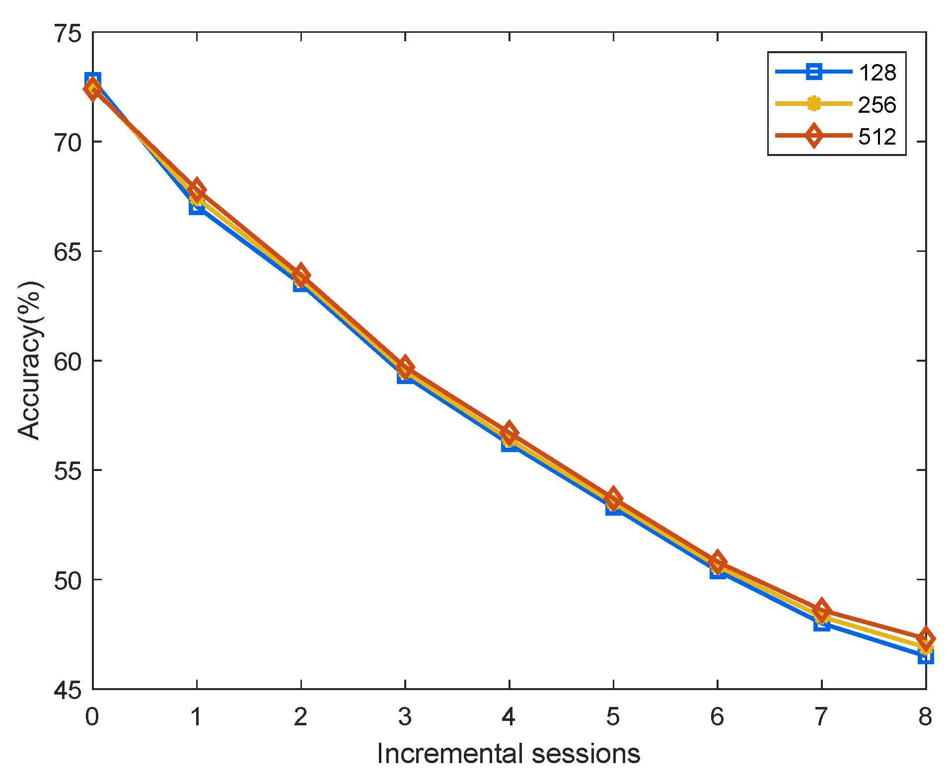
4.3.1. Effect of the Dimensionality of the Linear Mapping

This section further investigates how mapping features to different dimensions affects model performance. The ablation experiments are conducted on the miniImageNet dataset. Before transformation, the features extracted by the feature extractor are 512-dimensional. In the main experiments above, we adopted a 512-to-512 dimensional linear mapping. Here, we additionally evaluate two commonly used alternative dimensions: 512 to 256 and 512 to 128. As shown in Figure 6, the performance across different mapping dimensions is nearly identical. The trends and values of the three curves are very close. After analysis, we select the 512-to-512 mapping scheme due to its lower performance degradation over time. Although the 512-dimensional mapping performs slightly worse than the 256-dimensional mapping in the first session, it shows a slower decline in accuracy as the incremental sessions progress, resulting in the lowest overall performance degradation.

4.3.2. Effect of Different Few-Shot Tasks

We train and fine-tune the feature transformation layer using few-shot tasks sampled from the base dataset. Although the task scale during incremental learning is determined by the dataset (e.g., 5-way 5-shot), the task scale used to train the transformation layer can be manually configured since it is based on the base classes. The scale of few-shot tasks can influence the final performance of the model. In this section, we evaluate several commonly used few-shot task configurations on the miniImageNet dataset. The results are presented in

Table 4. Effect of different few-shot task scales on model performance.

Number of classes in the support set	5			10
Number of samples per class	1	5	10	1	5	10
Session 0	70.27	71.03	71.16	70.95	71.26	71.01
Session 8	45.40	46.22	46.75	45.77	47.00	46.84
Avg. accuracy	55.81	56.30	56.97	56.13	57.08	57.05
Performance degradation	24.87	24.81	24.41	25.18	24.26	24.17
Number of classes in the support set	15			20
Number of samples per class	1	5	10	1	5	10
Session 0	72.12	71.71	71.90	71.57	71.16	71.50
Session 8	47.27	47.11	47.37	46.15	46.95	47.28
Avg. accuracy	57.63	57.57	57.58	56.85	57.10	57.42
Performance degradation	24.85	24.60	24.53	25.42	24.21	24.22

, where the best value for each metric is highlighted in bold. The results show that the number of classes (ways) in the few-shot tasks has a more significant impact on performance compared to the number of support samples (shots) per class. When the number of classes is set to 15, the overall performance is the best. Specifically, under the 15-way setting, the 1-shot configuration yields the best performance in the first session and on average, while the 10-shot configuration achieves the best performance in the final session and exhibits the lowest performance degradation. After balancing performance and efficiency, we select the 15-way 1-shot task configuration. Under this setting, the model achieves competitive performance with fewer training samples and faster convergence.

4.3.3. Effect of Feature Transformation on Class Representations

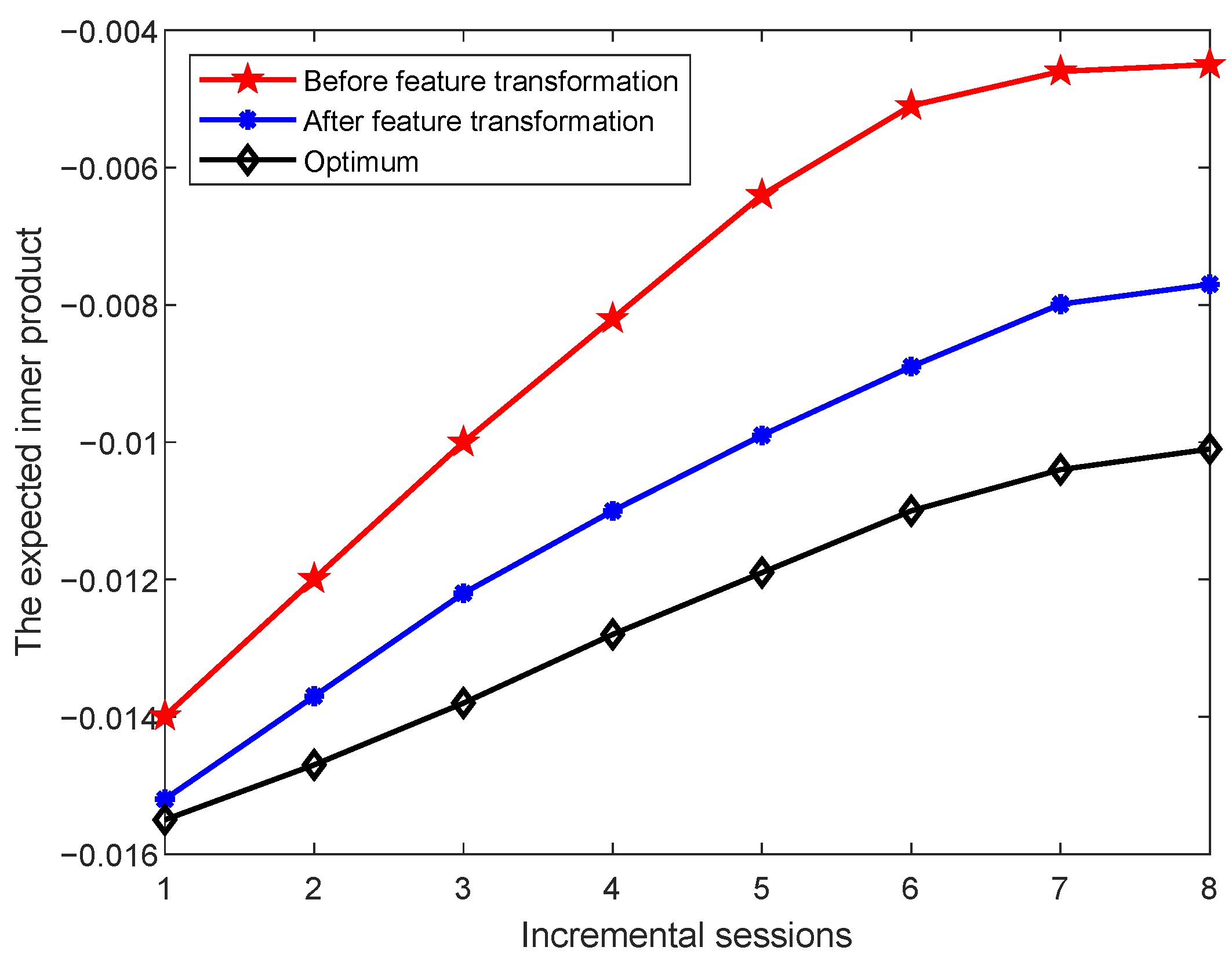
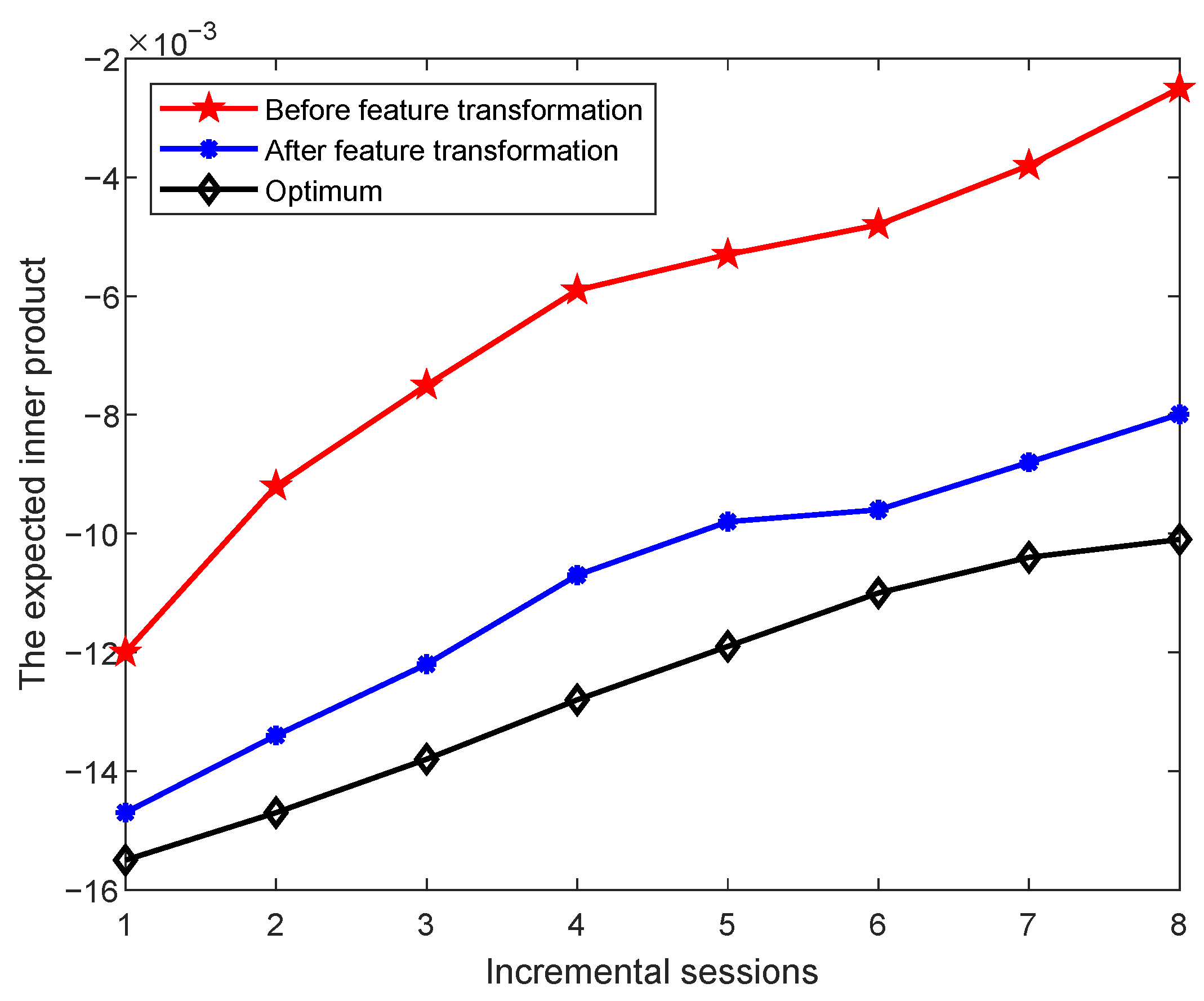
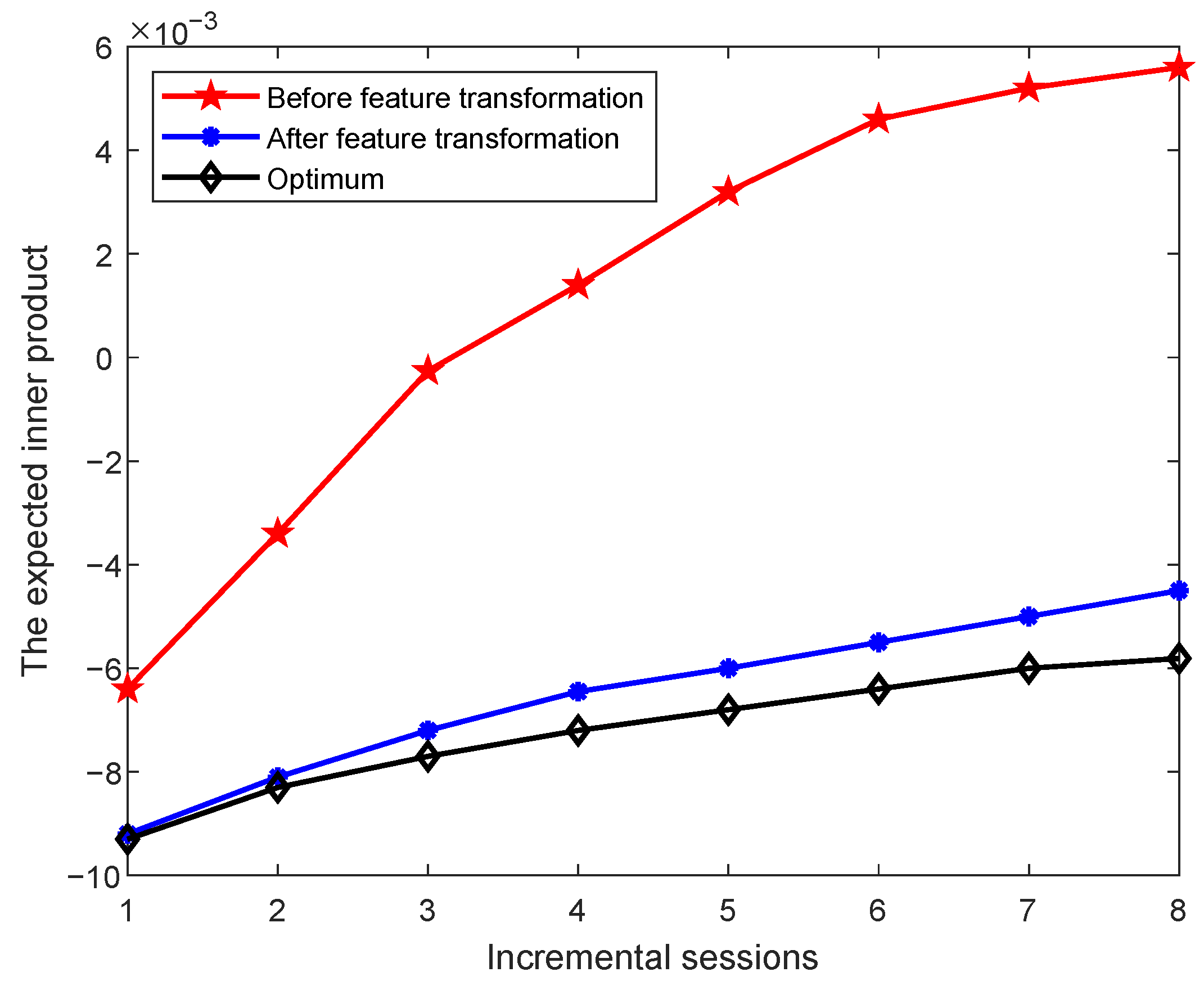
To validate the effectiveness of the proposed feature transformation, we further investigate the characteristics of the data before and after transformation. Specifically, we examine whether the class prototypes in each incremental session exhibit properties consistent with the neural collapse phenomenon, i.e., the expected inner product between any two distinct class mean vectors after centering. The expected inner products between class means are computed, and the results on the miniImageNet, CIFAR100, and CUB datasets are shown in Figure 7, Figure 8 and Figure 9, respectively.

An ideal set of class prototypes should satisfy the following property [14]: after centering and normalization, the inner product between any two distinct class means should equal $-1/(K-1)$, where K is the number of classes. This theoretical value increases as the number of classes increases. In the figures, the blue curve represents the theoretical optimum as the number of classes grows over the incremental sessions. The red and purple curves show the expected inner product values before and after feature transformation, respectively. We observe that after applying feature transformation, the expected inner product values between class centers move significantly closer to the theoretical optimum. This indicates that the transformation improves the relative positioning of class prototypes in the feature space, making them more aligned with the ideal distribution. This improved alignment is consistent with the key properties of neural collapse, particularly the tendency of class means to form equiangular configurations.

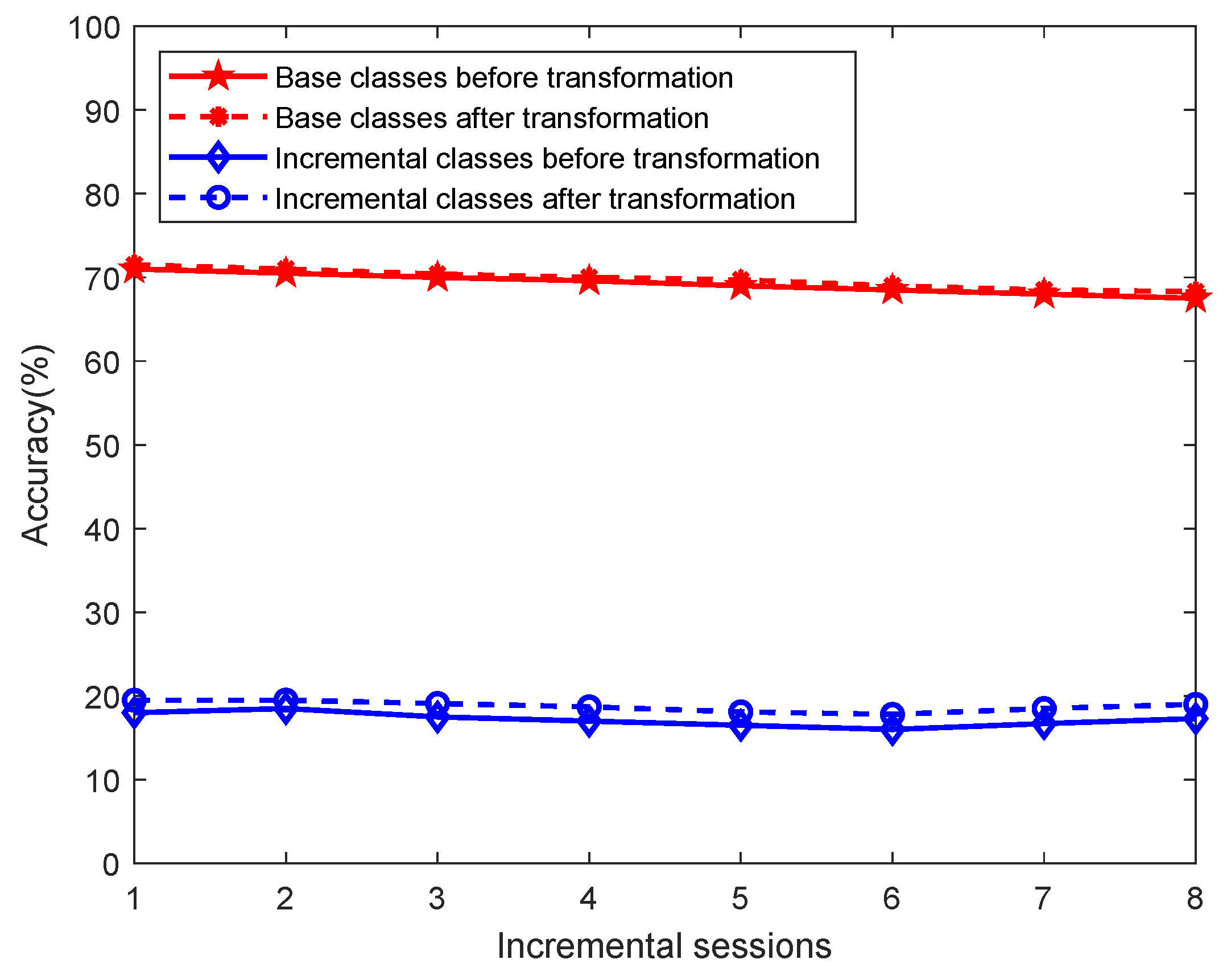
We further analyze the performance of base classes and newly introduced incremental classes throughout the learning process on miniImageNet as shown in Figure 10. The base class accuracy is calculated as the average accuracy over all base classes, while the incremental class accuracy is the average over all incremental classes learned up to the current session. The result shows that, regardless of whether feature transformation is applied, base classes consistently outperform incremental classes. This is primarily due to the fixed parameters of the feature extractor, which is trained solely on base class data and thus extracts more representative features for base classes. In contrast, features extracted for incremental classes are less representative, especially given the limited number of labeled samples used to estimate class prototypes, which introduces additional variance compared to full-data estimation. These two factors lead to the inferior performance of incremental classes during the learning process. However, the figure also reveals the practical benefit of our proposed feature transformation: it improves the performance of incremental classes while keeping the performance of base classes largely unaffected. In the transformed feature space, the gain in accuracy for incremental classes outweighs the minor drop in performance for base classes, resulting in an overall improvement in classification accuracy.

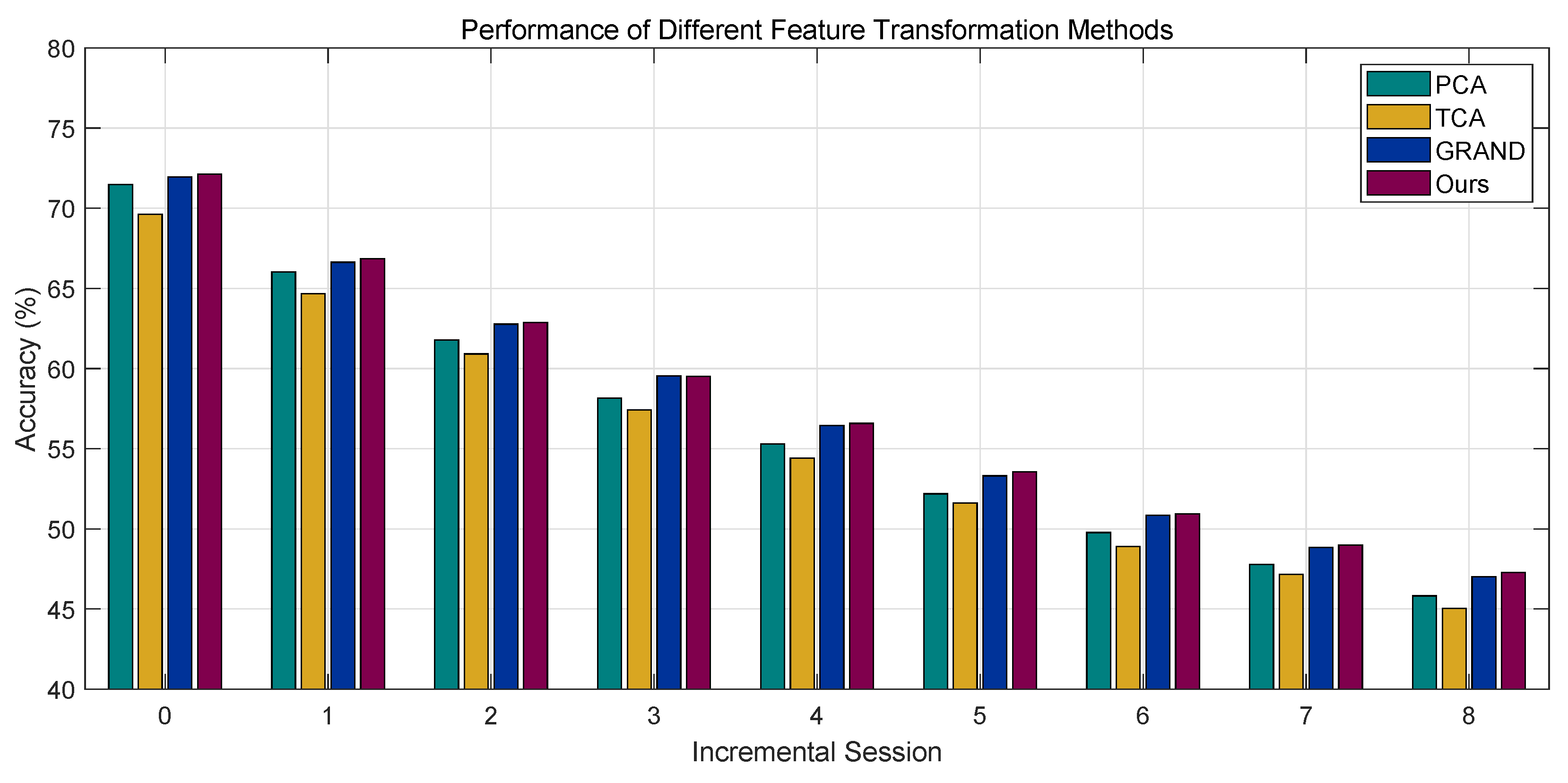
4.3.4. Comparison with Other Feature Transformation Methods

There exist various commonly used feature transformation methods, such as Principal Component Analysis (PCA), widely adopted for dimensionality reduction, and Transfer Component Analysis (TCA), frequently used in transfer learning. To validate that the proposed transformation method performs better under the constraint of a fixed feature extractor, we compare it with these alternative transformation methods in Figure 11. All methods use the same feature extractor with identical parameters for fair comparison.

PCA aims to reduce the dimensionality of the data while ensuring that the sample points remain well-separated in the new low-dimensional feature space. A common measure of separation is the covariance between vectors—when the covariance between two vectors in the transformed space is zero, they are considered completely uncorrelated, achieving the objective of separation. It is important to note that PCA involves centering the data by subtracting the mean. Therefore, if the test samples and class prototypes are jointly transformed via PCA, the distribution of test classes can significantly influence the resulting feature space. To avoid this issue, we apply PCA separately for each test sample and the class prototypes before performing classification. The original feature dimension is 512, and after PCA, the dimensionality is reduced to match the number of class prototypes available in the current session.

TCA is a classical method in transfer learning. It aims to minimize the Maximum Mean Discrepancy (MMD) between the marginal distributions of the source domain dataset $X_S$ and the target domain dataset $X_T$ through feature transformation:

$$\begin{array}{c}\hfill MMD(P_s\left(x\right),P_t\left(x\right))={\parallel {\displaystyle \frac{1}{|X_S|}}\sum _{i=1}^{|X_S|}\varphi \left(x_i\right)-{\displaystyle \frac{1}{|X_T|}}\sum _{j=1}^{|X_T|}\varphi \left(x_j\right)\parallel }_{{\mathcal{H}}_k}^2\end{array}$$

(4)

where ${\mathcal{H}}_k$ denotes a Reproducing Kernel Hilbert Space (RKHS) defined by a kernel function k. The mapping $\varphi (·)$ defines a transformation from the original data space to ${\mathcal{H}}_k$, where the kernel function corresponds to the inner product in the mapped space. In our experiments, we use the Gaussian (RBF) kernel with a kernel width of 1. When both the source and target domain data are specified, the TCA problem becomes an optimization problem that can be solved using the Lagrange dual method, without the need for gradient-based training. However, in incremental learning, there is no explicit target domain for domain adaptation. Upon analysis, we consider the maintained set of class prototypes to serve as a relatively good approximation of the target domain. The prototypes of the base classes are derived from pre-training and are thus highly representative. The prototypes of the novel classes are estimated as the mean of the support samples, representing the feature distribution of new classes after incremental updates. Therefore, the matrix formed by class prototypes after the i-th incremental session can be regarded as a good approximation of the target domain features. Since TCA is also a dimensionality reduction method, the dimension of the target feature space is set to the number of class prototypes available at the current stage.

In addition to PCA and TCA, we also compare with a recently proposed method named Graph Random Neural Networks (GRAND) [26]. From a structural perspective, GRAND combines a multilayer perceptron (MLP) with label propagation techniques. It includes additional mechanisms such as random feature dropout and propagation depth control, which contribute to its strong performance in graph-based tasks. In our implementation, the node features are extracted by the fixed feature extractor, edge weights are computed using cosine similarity between node pairs, and the propagation depth is set to 1.

The performance comparison among these methods is summarized in

Table 5. Performance degradation comparison on feature transformation methods.

Method	Performance Degradation
PCA	25.66
TCA	24.58
GRAND	24.94
Ours	24.85

. The results show that while TCA yields low performance degradation, this is primarily because it starts from a very low initial accuracy in the first session. In fact, TCA consistently achieves the lowest accuracy across all incremental sessions, making it the weakest performer overall. We believe this is due to the lack of an appropriately defined target domain. PCA achieves relatively high initial accuracy but suffers from significant degradation as the incremental learning process progresses. GRAND performs comparably to our proposed method, with slightly lower per-session accuracy and slightly higher degradation. The performance gap can be attributed to two main factors: (1) the MLP structure in GRAND acts as a more complex learnable transformation, and (2) the label propagation mechanism induces feature smoothing across samples, which can enhance overall stability but slightly compromise discriminability compared to purely feature-based transformation methods. Overall, our proposed feature transformation method demonstrates the best performance. It achieves consistently high accuracy across all incremental sessions while maintaining relatively low performance degradation.

5. Conclusions

This paper investigates the few-shot class-incremental learning and proposes a feature transformation method tailored for two-stage learning frameworks. Under the constraint of a fixed feature extractor, we sample various few-shot tasks from the base dataset to train a feature transformation module. Classification is then performed by comparing the transformed features of test samples with a maintained set of class prototypes. Experimental results demonstrate that the proposed method achieves strong performance across three benchmark datasets. It effectively improves the distribution of class prototypes, aligning them more closely with the ideal structure described by the neural collapse phenomenon. In addition, we explore the performance of other commonly used feature transformation methods under the two-stage training constraint. The results show that the proposed method is better suited for this framework and achieves the best performance among all evaluated transformation techniques.

Recent lightweight adaptation techniques, such as LoRA and Adapters, have shown strong performance in few-shot and incremental learning tasks by enabling efficient low-rank or bottleneck updates within frozen backbones. While our current design focuses on a standalone linear transformation layer, exploring the integration of these approaches with fixed feature extractors could be a promising direction for future work.