Dynamic Modeling and Validation of Peak Ability of Biomass Units

Abstract

Biomass units can play a certain role in peak summer and winter due to their advantages in terms of their environmental and short-term peak ability. To analyze the peak ability of biomass units, this paper focuses on the dynamic modeling of biomass unit peak ability. Firstly, the process of biomass feeding amount to power output is divided into a feed–heat module, heat–main steam pressure module and main steam pressure–power module. A two-input and two-output dynamic model is established where the feeding amount and turbine valve opening serve as inputs, and the main steam pressure and power serve as outputs. Then the effectiveness of the established model is validated by actual operation data of a 30 MW biomass unit. This dynamic model can provide a mechanistic model for analyzing the impact of fuel calorific value on the power output, and provide support for fuel management and scheduling strategies during the peak period of biomass units.

1. Introduction

The dual-peak characteristics of China’s power load during both winter and summer are becoming increasingly pronounced. The proportion of cooling load in summer and heating load in winter is increasing. In some provinces, the proportion of cooling load in summer to the maximum power load reaches 40–50%, or even more than 50%, and the power supply and demand are in tight balance [1]. Taking Henan Province as an example, the power security situation in Henan Province during peak summer is severe and complex. It is estimated that the maximum load of the Henan power grid this year is 83.5 million KW, an increase of 5.58 million KW year-on-year, an increase of 7.2%. This year, the peak gap is 7.5 million KW, and the power supply situation is grim. Due to the randomness, uncertainty, transients and other weather-dependent characteristics of renewable energy such as wind power and photovoltaics, the severe situation regarding the power supply is further increased. Due to their advantages of providing environmental protection and short-term peak ability (maximum power output), biomass generating units gradually play a certain role in summer and winter [2,3,4].

In recent years, the biomass industry at home and abroad has shown a sustained growth trend, and countries are competing to promote the introduction and innovation of biomass power generation technologies, such as biomass mixed combustion power generation and biomass gasification power generation. Among them, the Battelle Biomass Gasification Power Generation Demonstration Project in the United States represents the world’s most advanced level of biomass energy utilization. However, the high difficulty of using tar treatment technology and gas turbine transformation has limited the promotion process of commercial projects.

In order to analyze the peak ability of biomass units, it is necessary to establish a dynamic model from biomass fuel to unit load, to provide theoretical support for analyzing the peak ability of biomass units. At present, the research mainly focuses on the dynamic modeling of coal-fired units. Reference [5] established a model of 300 MW subcritical circulating fluidized bed units, which was verified by field data. Reference [6] established a dynamic model of “two-input and two-output” suitable for the direct energy balance control structure for a 300 MW subcritical pulverized coal boiler. Reference [7] considers the feed water heater system, bypass system and feed water pump, studies the dynamic mathematical model of coal-fired units suitable for fast cut-off technology, and verifies it at a 50% and 100% load. Reference [8] established the dynamic model of the steam turbine with condensing extraction back pressure and a combined cycle gas turbine, and studied the suppression mechanism of water level fluctuation and the design of a water level controller under transient switching mode. In Reference [9], a multi-input and multi-output dynamic model of the incinerator was established through image feature recognition and the transfer entropy algorithm. At present, there is little research on biomass combustion boilers. Because the biomass combustion mechanism is different from the coal combustion mechanism, the unit load and fuel composition have a great impact on the power generation efficiency of the whole power plant, and the dynamic model research needs to consider the different combustion characteristics. For biomass units, Reference [10] conducted a physical analysis of the combustion process in the furnace of a vibrating biomass grate furnace unit based on the combustion characteristics of biomass combustion, but is limited to the study of the combustion characteristics in the furnace. Reference [11] established the mathematical model and simulation model of biomass power plant combustion systems based on virtual data processing technology. Reference [12] carried out simulation research on a biomass vibrating grate, and analyzes and discusses the impact of grate vibration and fuel moisture fluctuation on boiler characteristics. Reference [13] established the fuel side combustion model of a biomass fluidized bed boiler through the energy conservation relationship, which provided a model basis for the design of its coordinated control system. However, current modeling research on biomass units predominantly focuses on the combustion process in the furnace and lacks research on the unit output, especially for the dynamic modeling of biomass grate furnace units. This is unfavorable for analyzing the peak ability of biomass units.

To better analyze the peak ability of the biomass grate boiler unit, according to the characteristics of the biomass grate boiler unit, the process from the biomass unit feed quantity to the unit power is divided into the feed–heat module, the heat–main steam pressure module and the main steam pressure–power module. A “two-input and two-output” dynamic model with the feed quantity and the turbine valve opening as the input and the main steam pressure and turbine output power as the output is established, which is verified by the actual operation data of a 30 MW biomass grate boiler unit. The dynamic model can provide a mechanism model for analyzing the impact of fuel calorific value on unit power, and provide support for a fuel management and scheduling strategy during the peak period of biomass grate furnace units.

This paper first introduces the production process of the biomass power plant, and then establishes the dynamic models of feed–heat, heat–main steam pressure and main steam pressure–power based on energy conservation. Then the effectiveness of the dynamic model is validated by comparing actual operation data and analyzing the open-loop step response characteristics. Finally, the paper summarizes the work of the full text.

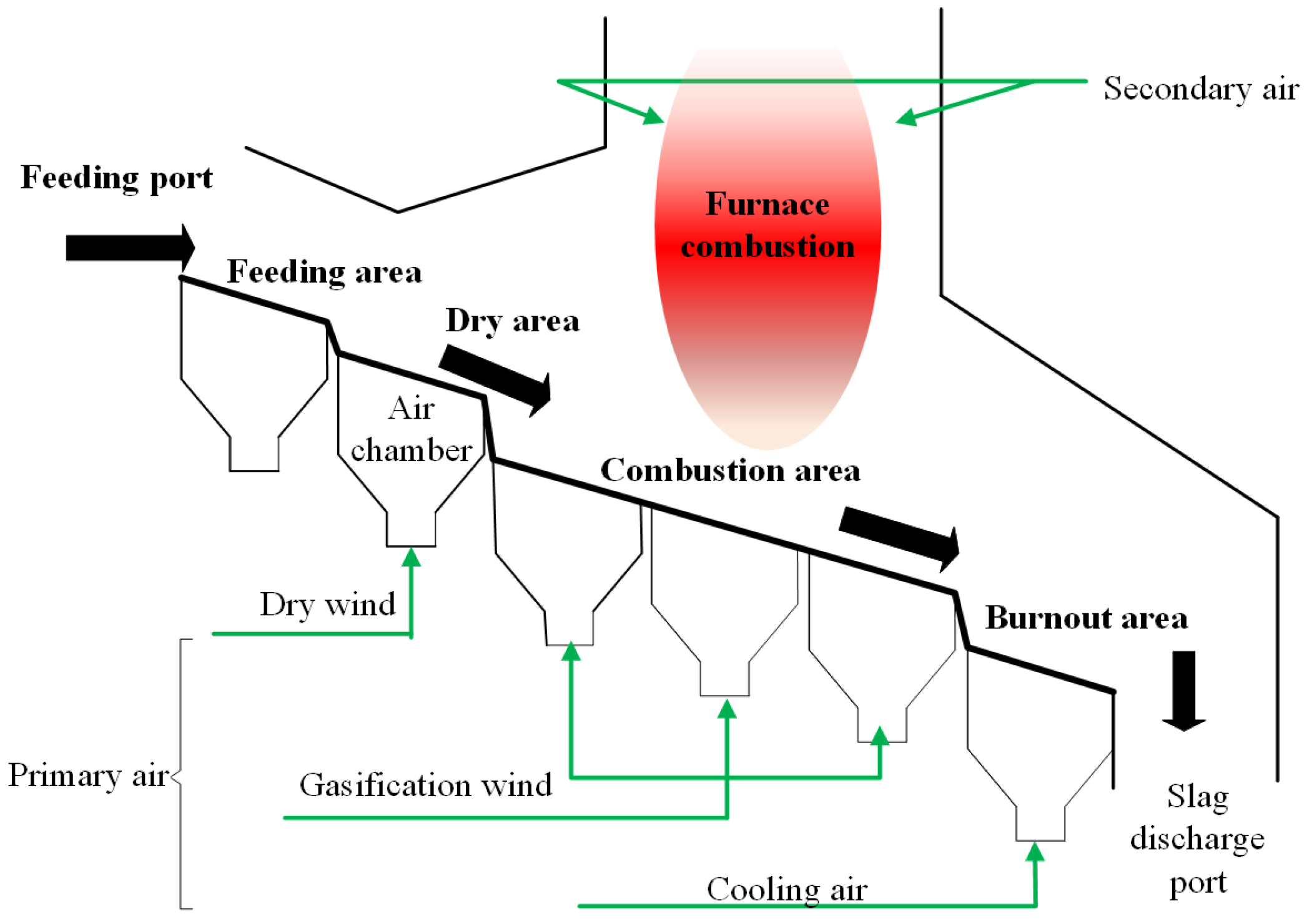
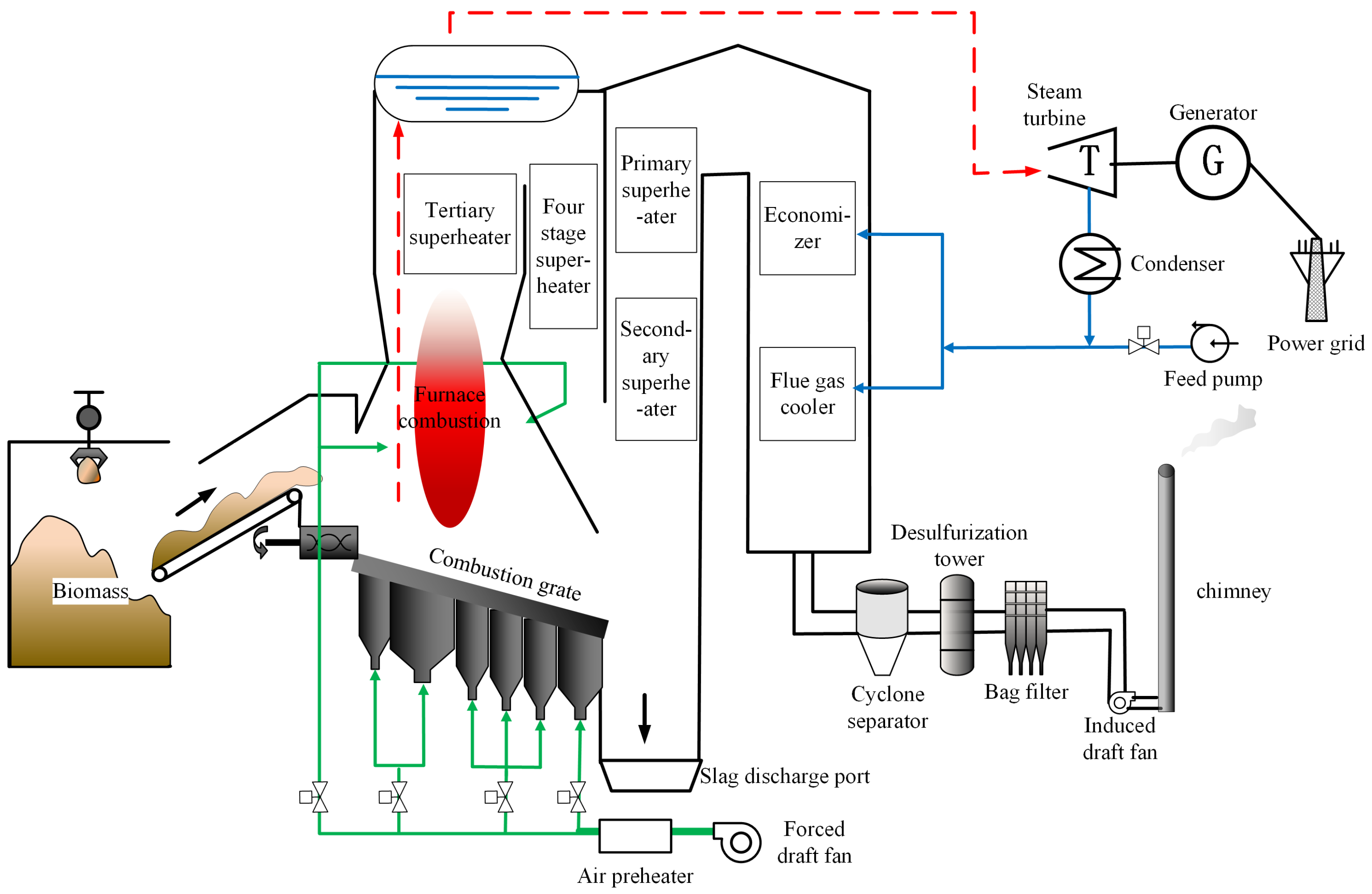
2. Biomass Power Generation Process

This paper studies the biomass unit based on the grate combustion furnace. Its structure is shown in Figure 1. The grate combustion furnace is composed of reciprocating parts with a certain inclination angle, which is divided into three areas. Among them, the first part is the dry area. The biomass fuel gradually heats up through the heat conduction and radiation of the top heat source, and then releases water. The second part is the combustion area, where volatile gas and fixed carbon begin to burn and the temperature in the furnace rises rapidly. With the continuous increase in temperature, the combustible gas in the fuel gradually precipitates due to the thermal effect and diffuses upward with the primary air blowing in. The third part is the burnout area, where the fixed carbon is completely burned and finally turned into ash and slag, which is discharged from the slag discharge port [14,15,16].

The core hardware of a biomass power plant boiler includes a furnace, superheater, flue, reheater, air preheater and other auxiliary equipment. The production process of biomass grate furnaces is shown in Figure 2, which is mainly divided into three key stages.

First, biomass fuel needs to be pretreated [17]. This link involves the crushing and drying of collected straw, peanut shell, sawdust and other materials to ensure that the fuel meets the particle size and moisture standards suitable for combustion, so as to improve its combustion efficiency. Pretreatment cannot only improve the combustion performance of fuel but also directly affect the overall operation efficiency and economic benefits of biomass power plants. The treated fuel is then stored and transported to the boiler. In the warehouse, the fuel is properly stored for daily production. During production, the staff accurately grab an appropriate amount of fuel with a professional large grab and place it on the feeding conveyor belt. With the operation of the belt, the fuel is delivered to the furnace. Then, it enters the combustion control phase. To ensure the best combustion effect, it is necessary to accurately control the key parameters such as the combustion temperature, air supply volume and water supply flow. Finally, it goes through the heat collection and tail gas treatment. The heat energy generated by combustion is converted into steam, which drives the steam turbine to generate electricity, realizing the energy-efficient conversion of biomass units.

3. Dynamic Modeling of Biomass Unit Peak Ability

This section describes the combustion system through differential equations. Based on the first principle of mass conservation and energy conservation, the biomass power plant system is divided into three models for modeling and analysis.

3.1. Feed–Heat Model

The particle size of biomass fuel is uneven, the density distribution is different, and the fuel composition is complex [18]. It is difficult to detect the feeding amount of the boiler online, so it is necessary to estimate the feeding amount of the boiler. In addition, the transmission of feed on the belt has certain delay characteristics, so the transmission process can be approximated by a pure delay link. Assuming the type and density of fuel remain unchanged, the fuel quantity $F_b$ (kg/s) in the boiler is

$$\begin{array}{c}\hfill F_b\left(t\right)=K_1{\mu }_B\left(t-\tau \right),\end{array}$$

(1)

where ${\mu }_B\left(t\right)$ (kg/s) is the fuel quantity entering the furnace at a certain time. $K_1$ is the proportional coefficient, and $K_1=1$ is taken for simple calculation. The delay time $\tau$ is related to the belt structure.

The fuel fed into the grate boiler needs to be gradually distributed over the moving grate and combusted in stages and zones, rather than being burned immediately [19]. Therefore, there is a certain amount of fuel stored on the combustion grate, and the newly added fuel and the fuel consumed by combustion reach a new balance. According to the law of the conservation of mass,

$$\begin{array}{c}\hfill c_1{\displaystyle \frac{\mathrm{d}B\left(t\right)}{\mathrm{d}t}}=F_b\left(t\right)-B_r\left(t\right)(1-A_{ar})-D_{ash},\end{array}$$

(2)

where $c_1$ is the dynamic parameter to be identified. $B\left(t\right)$ (kg) is the current total fuel quantity of the grate. $B_r\left(t\right)$ (kg/s) is the combustion rate of the furnace fuel. $A_{ar}$ (%) is the mass fraction of the received base ash of biomass fuel, and $A_{ar}=13.73\%$ is taken for simple calculation. $D_{ash}$ (kg/s) is the amount of slag discharged. Due to the low ash content of biomass fuel and the small amount of residual residue after fuel combustion [20], the effect of the slag discharge amount $D_{ash}$ will not be considered in this model. Equation (2) can be simplified as

$$\begin{array}{c}\hfill c_1{\displaystyle \frac{\mathrm{d}B\left(t\right)}{\mathrm{d}t}}=F_b\left(t\right)-B_r\left(t\right)(1-A_{ar}).\end{array}$$

(3)

The fuel combustion rate $B_r\left(t\right)$ is affected by the total amount of fuel on the grate, the oxygen concentration and the furnace temperature [21]. $B_r\left(t\right)$ is decided by

$$\begin{array}{c}\hfill B_r\left(t\right)=k_r{C}_{O_2}B\left(t\right)k_s,\end{array}$$

(4)

where $k_r$ is the combustion coefficient. $C_{O_2}$ (mol/${\mathrm{m}}^3$) is the oxygen concentration. $k_s$ is the combustion reaction rate coefficient, which is a function of the oxygen diffusion rate $k_g$, fuel chemical reaction rate $k_c$ and ash layer diffusion mass transfer resistance coefficient $k_a$ [22]. In order to simplify the calculation, the influence of $k_a$ on $k_s$ is not considered temporarily, that is

$$\begin{array}{c}\hfill k_s={\displaystyle \frac{1}{(\frac{1}{k_g}+\frac{1}{k_c})}}={\displaystyle \frac{1}{(\frac{d_c}{sh{D}_g}+\frac{1}{k_c})}},\end{array}$$

(5)

where $sh$ is the Sherwood number. $D_g$ (${\mathrm{m}}^2$/s) is the oxygen diffusion coefficient and $d_c$ (m) is the average particle size.

In practical application, $k_s$ can be determined through the empirical formula proposed by Nauze [23],

$$\begin{array}{c}\hfill k_c=AT{e}^{-E/\left(RT\right)},\end{array}$$

(6)

where A is the frequency factor. T (K) is the furnace temperature. E (kJ/mol) is the apparent activation energy. R (kJ/(mol·K)) is the gas constant.

The oxygen concentration $C_{O_2}$ is proportional to the total air supply volume $A_{ir}$. The unit load will affect the total air volume and oxygen concentration in the furnace, so the oxygen concentration calculation formula is

$$\begin{array}{c}\hfill C_{O_2}=K_{O_2}{A}_{ir}=k_{O_2}{N}_e\left(t\right)A_{ir},\end{array}$$

(7)

where $K_{O_2}$ is the relationship coefficient between oxygen concentration and total air supply volume. $A_{ir}$ (${\mathrm{m}}^3$/s) is the total air supply volume under the standard state, which is composed of primary air and secondary air. $k_{O_2}$ is the correction factor. $N_e\left(t\right)$ (MW) is the unit load.

Further, Equation (3) can be written as

$$\begin{array}{c}\hfill c_1{\displaystyle \frac{\mathrm{d}B\left(t\right)}{\mathrm{d}t}}=K_1{\mu }_B\left(t-\tau \right)-K_2{N}_e\left(t\right)B\left(t\right)(1-A_{ar}),\end{array}$$

(8)

where $K_2$ is the static parameter to be identified.

The heat source inside the furnace is mainly the combustion heat of biomass fuel. Ignoring the convective heat transfer inside the furnace, the total heat $Q_r\left(t\right)$ released at time t can be obtained based on the law of the conservation of energy,

$$\begin{array}{c}\hfill c_2{\displaystyle \frac{\mathrm{d}{Q}_r\left(t\right)}{\mathrm{d}t}}=B_r\left(t\right)Q_{net}-Q_r\left(t\right)=K_2{D}_{T}B\left(t\right)Q_{net}-Q_r\left(t\right),\end{array}$$

(9)

where $Q_{net}$ is the calorific value of biomass combustion. $c_2$ and $K_3$ are the dynamic and static parameters to be identified, respectively. The relationship between steam turbine flow $D_T$ and power $N_e$ will be be presented in the subsequent section.

During the actual operation of the unit, the heat absorbed by the water wall $Q_t\left(t\right)$ is related to the unit load $N_e\left(t\right)$ [24],

$$\begin{array}{c}\hfill Q_t\left(t\right)=K_4{N}_e\left(t\right),\end{array}$$

(10)

where $K_4$ is the ratio coefficient. Since the load fluctuation of the biomass unit is small, it can be set as a constant over a long period for simple calculation [25]. $K_4$ is the static parameter to be identified.

In conventional practice, the temperature of the bed material within the furnace’s dense-phase region is considered equivalent to the furnace temperature. Based on the principle of energy balance,

$$\begin{array}{c}\hfill C_s{M}_s{\displaystyle \frac{\mathrm{d}T\left(t\right)}{\mathrm{d}t}}=Q_r\left(t\right)-Q_t\left(t\right)-△h_{air}{A}_{ir}-Q_{pz},\end{array}$$

(11)

where $C_s$ (MJ/(kg·°C)) is the heat capacity of the bed material. $M_s$ (kg) is the amount of bed material in the furnace. $△h_{air}$ (MJ/${\mathrm{m}}^3$) is the change in air volume enthalpy. $△h_{air}{A}_{ir}$ (MJ) is the heat taken away by the flue gas flow. $Q_{pz}$ (MJ) is the heat taken away by the slag discharge flow. Considering that the heat taken away by the flue gas flow and slag discharge flow exhibits a positive correlation with the furnace temperature [26] gives

$$\begin{array}{c}\hfill c_3{\displaystyle \frac{\mathrm{d}T\left(t\right)}{\mathrm{d}t}}=Q_r\left(t\right)-Q_t\left(t\right)-K_{5}T\left(t\right),\end{array}$$

(12)

where $c_3$ and $K_5$ are the dynamic and static parameters to be identified, respectively.

The process where the total heat released above is absorbed by water and steam takes a certain time, so the heat absorbed by the waterside is

$$\begin{array}{c}\hfill c_4{\displaystyle \frac{\mathrm{d}Q\left(t\right)}{\mathrm{d}t}}=Q_r\left(t\right)-Q_t\left(t\right)-Q\left(t\right),\end{array}$$

(13)

where $Q\left(t\right)$ (MJ) is the heat absorbed by water and steam. $c_4$ is the dynamic parameter to be identified.

3.2. Heat–Pressure Model

Assuming that the feed water control system of the biomass unit can keep the water level in the drum unchanged, and the steam temperature and feed water temperature remain stable, the steam flow of the drum is approximately [5],

$$\begin{array}{c}\hfill D_b\left(t\right)\approx Q\left(t\right)/r_s,\end{array}$$

(14)

where $D_b\left(t\right)$ (kg/s) is the steam flow from the drum. $r_s$ (MJ/kg) represents the latent heat of vaporization. For simplified calculation, $r_s\approx 1.0$ MJ/kg is adopted as the assumed value.

In this model, the steam-side temperature of the drum and the temperature variations in the superheated pipe are ignored. According to the calculation method of the drum boiler in Document [27], it can be obtained that,

$$\begin{array}{c}\hfill {\displaystyle \frac{\mathrm{d}{P}_b}{\mathrm{d}t}}=(D_b-D_s)/C_b,\end{array}$$

(15)

$$\begin{array}{c}\hfill D_s=\sqrt{\left(P_{\mathrm{b}}-P_{\mathrm{T}}\right)/r_{\mathrm{s}}},\end{array}$$

(16)

$$\begin{array}{c}\hfill {\displaystyle \frac{\mathrm{d}{P}_T}{\mathrm{d}t}}=(D_s-D_T)/C_m,\end{array}$$

(17)

where $P_b$ (Mpa) is the boiler drum pressure. $D_s$ (kg/s) is the main steam flow. $P_T$ (Mpa) is the main steam pressure. $C_b$ and $C_m$ are the thermal storage coefficient of the evaporative surface and the capacity coefficient of the steam pipeline, respectively. $C_b$ means the amount of steam generated by the heat absorbed or released by the evaporation surface system when the evaporation surface pressure changes by 1 MPa. In the actual operation process, when the pressure changes little, it can be regarded as a constant. As the medium in the main steam pipe is single-phase superheated steam, its heat storage capacity is limited, so the capacity coefficient of the steam pipe is far less than the thermal storage coefficient of the evaporative surface [12]. From the above Equations (15)–(17), the simplified formula of this part of the model can be derived as follows:

$$\begin{array}{c}\hfill c_5{\displaystyle \frac{\mathrm{d}{P}_b\left(t\right)}{\mathrm{d}t}}=Q\left(t\right)-K_6\sqrt{P_b\left(t\right)-P_T\left(t\right)},\end{array}$$

(18)

$$\begin{array}{c}\hfill c_6{\displaystyle \frac{\mathrm{d}{P}_T\left(t\right)}{\mathrm{d}t}}=K_7\sqrt{P_b\left(t\right)-P_T\left(t\right)}-D_T\left(t\right),\end{array}$$

(19)

where $K_6$ and $K_7$ are the static parameters to be identified. $c_5$ and $c_6$ are dynamic parameters to be identified.

3.3. Pressure–Power Model

It is assumed that the regulating stage pressure of steam turbines is directly proportional to the product of the main steam pressure and the steam turbine valve opening. Under stable conditions, the regulating stage pressure of steam turbines can be described by the following formula,

$$\begin{array}{c}\hfill P_1=K_8{\mu }_T{P}_T,\end{array}$$

(20)

where $P_1$ (Mpa) is the pressure of the regulating stage. ${\mu }_T$ (%) is the opening of the steam turbine valve. $K_8$ is the static parameter to be identified. The dynamic expression of Equation (20) is

$$\begin{array}{c}\hfill c_7{\displaystyle \frac{\mathrm{d}{P}_1\left(t\right)}{\mathrm{d}t}}=K_8{\mu }_T\left(t\right)P_T\left(t\right)-P_1\left(t\right),\end{array}$$

(21)

where $c_7$ is the dynamic parameter to be identified.

The steam flow of the steam turbine and the pressure of the governing stage can be approximately linear [28], and its dynamic expression is

$$\begin{array}{c}\hfill c_8{\displaystyle \frac{\mathrm{d}{D}_T\left(t\right)}{\mathrm{d}t}}=K_9{P}_1\left(t\right)-D_T\left(t\right),\end{array}$$

(22)

where $c_8$ and $K_9$ are the dynamic and static parameters to be identified, respectively.

During normal operation, the steam flow rate of the steam turbine $D_T\left(t\right)$ determines the efficiency of the steam turbine and the power of the generator [29],

$$\begin{array}{c}\hfill N_e=K_{10}{D}_T\left(t\right)\end{array}$$

(23)

where $N_e$ (MW) is the output power of the steam turbine. $K_{10}$ is the static parameter to be identified.

To sum up, the feed–heat module, heat–pressure module and pressure–power module of a biomass power plant can be described by the following formulas:

$$\begin{array}{c}\hfill \left\{\begin{array}{c}{\displaystyle \frac{\mathrm{d}B\left(t\right)}{\mathrm{d}t}}={\displaystyle \frac{1}{c_1}}(K_1{\mu }_B\left(t-\tau \right)-K_2{N}_e\left(t\right)B\left(t\right)(1-A_{ar}))\hfill \\ {\displaystyle \frac{\mathrm{d}{Q}_r\left(t\right)}{\mathrm{d}t}}={\displaystyle \frac{1}{c_2}}(K_3{N}_e\left(t\right)B\left(t\right)-Q_r\left(t\right))\hfill \\ {\displaystyle \frac{\mathrm{d}T\left(t\right)}{\mathrm{d}t}}={\displaystyle \frac{1}{c_3}}(Q_r\left(t\right)-K_4{N}_e\left(t\right)-K_{5}T\left(t\right))\hfill \\ {\displaystyle \frac{\mathrm{d}Q\left(t\right)}{\mathrm{d}t}}={\displaystyle \frac{1}{c_4}}(Q_r\left(t\right)-K_4{N}_e\left(t\right)-Q\left(t\right))\hfill \end{array}\right.\end{array}$$

(24)

$$\begin{array}{c}\hfill \left\{\begin{array}{c}{\displaystyle \frac{\mathrm{d}{P}_b\left(t\right)}{\mathrm{d}t}}={\displaystyle \frac{1}{c_5}}(Q\left(t\right)-K_6\sqrt{P_b\left(t\right)-P_T\left(t\right)})\hfill \\ {\displaystyle \frac{\mathrm{d}{P}_T\left(t\right)}{\mathrm{d}t}}={\displaystyle \frac{1}{c_6}}(K_7\sqrt{P_b\left(t\right)-P_T\left(t\right)}-D_T\left(t\right))\hfill \end{array}\right.\end{array}$$

(25)

and

$$\begin{array}{c}\hfill \left\{\begin{array}{c}{\displaystyle \frac{\mathrm{d}{P}_1\left(t\right)}{\mathrm{d}t}}={\displaystyle \frac{1}{c_7}}(K_8{\mu }_T\left(t\right)P_T\left(t\right)-P_1\left(t\right))\hfill \\ {\displaystyle \frac{\mathrm{d}{D}_T\left(t\right)}{\mathrm{d}t}}={\displaystyle \frac{1}{c_8}}(K_9{P}_1\left(t\right)-D_T\left(t\right))\hfill \\ N_e\left(t\right)=K_{10}{D}_T\left(t\right)\hfill \end{array}\right.\end{array}$$

(26)

Remark 1.

Based on the discussions above, one can learn that this model is based on first principles, where the biomass power plant system is divided into three processes, the feed–heat process, heat–pressure process and pressure–power process. Note that the dynamic parameters $c_1$–$c_4$ represent the inertia time constant of the first module, $c_5$–$c_6$ correspond to the second module and $c_7$–$c_8$ are associated with the third module. These dynamic parameters represent the thermal inertia of biomass boilers, which could limit the ramp rate.

4. Dynamic Model Validation

For the dynamic model of the peak ability of biomass generating units in Equations (24)–(26) established in the previous section, this section identifies the static and dynamic parameters based on the operation data of a 30 MW biomass generating unit. In addition, it is established and validated on the MATLAB R2021a and Simulink platforms.

In addition, the unit uses biomass as fuel, and the particle size of the fuel entering the furnace is less than 150 mm. The received ash content of biomass fuel is 13.73%, and its volatile matter mass fraction is relatively high, that is, the carbon mass fraction of combustion is low. The industrial analysis of biomass fuel is shown in

Table 1. Industrial analysis of biomass fuel.

Fuel Name	Average Moisture Content (%)	Average Ash Content (%)	Calorific Value (kcal)
Peanut Shell	15.53	17.63	3100.63
Wheat Straw	18.75	13.89	2758.72
Wheat Husk	9.39	20.02	2805.56
Bark	43.28	14.80	2000.44
Whole Template			3350
Waste Veneer Strip	15.84	5.42	3329.15
Corn Straw	14.66	21.85	2500.07
Chili Stalks	18.83	10.32	3044.81
Corncob	18.98	3.52	3222.11
Branch	37.42	8.77	2278.48

.

4.1. Data Preprocessing

There is variability in the operation of the on-site unit, especially the instantaneous value of the feed rate, which is due to the sharp fluctuation in the value caused by the accuracy problem of the measuring device. The maximum value can reach 86.9361 kg/s, while the minimum value is only 0.05 kg/s. During the actual operation of the unit, the feed volume should not fluctuate so much. To filter the data effectively, the median filter processing method is used. The comparison is shown in Figure 3. The data cleaning after median filtering has achieved remarkable results to guarantee the veracity and robustness of the dataset. It is worth noting that the feed volume maintains good consistency in the noninput stage, indicating that the filtering process does not distort the natural characteristics of the data. In addition, the filtered feed rate curve is smoother, making the feed rate more reasonable.

4.2. Model Validation

To verify the model’s accuracy, this paper uses the historical data of a biomass unit for experiments. The collection time is from 00:00:00 to 24:00:00 on 20 March 2024. A group of data is sampled every second, and a total of 86,401 groups of data are collected. The data is divided into several sections, and the static and dynamic parameters are identified and verified. The static parameters are obtained through the calculation of the steady-state operation data of the unit, as shown in

Table 2. Static parameter values.

Steady State Parameters	Numerical Value
$K_1$	1.0000
$K_2$	6.8143 × 10−6
$K_3$	7.1550 × 10−5
$K_4$	1.1500
$K_5$	0.0615
$K_6$	63.6531
$K_7$	39.7832
$K_8$	0.0082
$K_9$	5.6358
$K_{10}$	0.8758

.

Root mean square error (RMSE) and mean absolute error (MAE) are adopted to evaluate the prediction accuracy of the constructed model for main steam pressure and unit output power. RMSE is the square of the deviation between the model output and the real value, which can show the degree of fitting between the model output and the actual output well. MAE measures the overall deviation in a model’s predictions by calculating the average absolute error between the predicted and true values. The calculation method is as follows:

$$\begin{array}{c}\hfill RMSE=\sqrt{{\displaystyle \frac{1}{n}}{\displaystyle \sum _{i=1}^n}{(y_i-y_i^{\ast })}^2}\end{array}$$

(27)

$$\begin{array}{c}\hfill MAE={\displaystyle \frac{1}{n}}{\displaystyle \sum _{i=1}^n}|y_i-y_i^{\ast }|\end{array}$$

(28)

where $y_i$ is the actual value of main steam pressure or turbine output power data, while $y_i^{\ast }$ is the output value of the model main steam pressure or turbine output power.

The dynamic parameters and delay time constants obtained by the empirical trial and error method are shown in

Table 3. Dynamic parameter identification results.

Dynamic Parameters	Numerical Value
$c_1$	80.0000
$c_2$	0.4100
$c_3$	148.5761
$c_4$	0.4523
$c_5$	31.9593
$c_6$	37.5900
$c_7$	1.8463
$c_8$	1.0325
$\tau$	10.0000

.

Based on the identified dynamic model, the comparison of model outputs with actual operation data under the same excitation can be obtained, as shown in Figure 4. The distribution of model error over time is shown in Figure 5.

Compared with Figure 3 and Figure 4a, it can be seen that at several key periods, such as 500 s, 2000 s and 5000 s, when the feeding amount stops input, the power output also decreases, but it is not difficult to find that there is a certain lag. The feed rate is the energy input source of the biomass unit, which directly causes the fuel supply in the combustion chamber to stop and the heat generation to reduce. Because the combustion process takes time, the heat output will not respond immediately, but there is a certain delay. The decrease in heat will reduce the steam generation in the boiler and the main steam pressure, which will lead to the weakening of steam power to drive the steam turbine and the reduction in output power. In addition, due to the existence of the combustion process, boiler thermal inertia and turbine mechanical inertia, the power reduction is not instantaneous but a gradual process. This phenomenon reflects the dynamic balance relationship between energy input and output, and conforms to the physical law of biomass units. It can be considered that the model has high mechanism rationality.

Figure 4 represents that the power output change trajectory of the model established in this paper is almost consistent with the actual operation data. The prediction performance of power output shows a good follow-up ability, which accurately reflects the dynamic change trend in the actual operation. However, the prediction effect of the main steam pressure circuit is slightly inferior to that of the power output circuit, but it can still be seen from the figure that its change trend is significantly similar to the actual operation data in the key decline range. The proposed model successfully captures the dominant trends, thereby demonstrating its capability to accurately characterize the operational dynamics of biomass-fired power units under varying working conditions. The error distribution diagram is shown in Figure 5, from which we can see that the dynamic error of the power circuit is within ±5% and the dynamic error of the main steam pressure circuit is within ±10% within the time range of nearly 2 h. The average dynamic error of the power loop of the dynamic model is 3.93%, and the maximum is less than 5%. The error is in the ideal acceptable range.

To validate the model’s effectiveness, operational data from multiple operational periods were utilized to constitute the test set. By comparing the actual operation data with the output of the model under corresponding working conditions, the comparison results and the distribution of model error with time are shown in Figure 6. The model demonstrates that the output is consistent with the actual operation data, and its dynamic error range is stable between 5% and 10%. The results show that the established model has high accuracy and can accurately reflect the dynamic characteristics of the system when the feed rate or the valve opening of the steam turbine changes, providing reliable support for system optimization and unit peak ability analysis.

It should be noted that the dynamic parameter identification in Table 3 is obtained by the empirical trial and error method. On this basis, the RMSE values of the power circuit and the main steam pressure circuit are 0.2201 and 0.4655, respectively, while the corresponding MAE values are 0.1520 and 0.4017. The parameters can also be further optimized by the NSGA-II (Non-dominated Sorting Genetic Algorithm II) with Equation (27) as the optimization objective [30]. The optimization framework utilizes a binary-coded representation alongside a tournament selector. This approach maintains population diversity while identifying elite individuals. Key parameter configurations are as follows: the population size is set at 50, the number of iterations is 20 and other settings remain at their default values. Figure 7 shows the Pareto front of the non-dominated solution. The points indicated by the arrow in the graph are selected from the Pareto front and the corresponding dynamic parameters determined are given in

Table 4. Dynamic parameter identification results based on NSGA-II.

Dynamic Parameters	Numerical Value
$c_1$	51.3606
$c_2$	4.1577
$c_3$	225.2294
$c_4$	0.6818
$c_5$	32.6523
$c_6$	25.9014
$c_7$	2.1168
$c_8$	1.3462
$\tau$	16.1684

. Based on it, the results shown in Figure 8 can be obtained. The figure shows that the output of the model is consistent with the actual operation data, and its dynamic error range is stable within 5% and 10%. The RMSEs of the power circuit and the main steam pressure circuit after using the multi-objective evolutionary algorithm are 0.2707 and 0.4841, respectively. Generally, the RMSE values of the load circuit and the main steam pressure circuit are between 0.2∼0.5 and it can be considered that the model can accurately predict the data.

This study uses the NSGA-II to optimize the model parameters. The RMSE index is in a reasonable range, which reflects the value of the algorithm in multi-objective optimization. However, compared with the empirical trial and error method, the optimized model has the problem of output oscillation under complex conditions. The algorithm does not fully consider the output stability and generalization ability when optimizing the RMSE index. Nevertheless, the parameter solution generated by the NSGA-II provides a key reference for the empirical trial and error method, helps to delimit the parameter debugging interval and significantly improves the debugging efficiency. In the future, the output stability constraint can be added to the algorithm, and the guiding effect of the algorithm on the empirical trial and error method can be quantified to further tap the potential of collaborative optimization of the two methods.

Open-loop verification was performed on the established model. Step changes were applied to the input variables at the selected time point of 2000 s. The feed rate input and valve opening changed to 90%, 95% and 115% of the original value, respectively. The input changes are shown in Figure 9, and the results are shown in Figure 10 and Figure 11.

Due to the large fluctuation in the feeding amount, the system is relatively stable after 2000 s (about 5000 s as shown in Figure 6). During this period, the average feeding amount is 7.7322 kg/s, which can be used as the initial value of the step response of the steady-state system. When the feed input becomes smaller, the fuel supply will be reduced and the heat energy released by combustion will be reduced. Then the steam generation rate will be reduced, and the main steam pressure will gradually decrease due to the reduction in steam generation. Especially in the open-loop system with open-loop control, the pressure will continue to decrease until a new thermal balance is reached. On the other hand, the output power is limited by the reduction in thermal energy input, and the power of the steam turbine weakens, showing a downward trend. Otherwise, the main steam pressure and output power will rise.

The decrease in valve opening will increase the steam outflow resistance and reduce the steam flow, which will affect the steam pressure and combustion efficiency. The fuel input (thermal energy generation) of the boiler remains unchanged, that is, the steam generation rate remains unchanged. When the outflow decreases due to the decrease in the valve opening, the steam accumulates in the pipeline, resulting in the rise of the main steam pressure until it reaches a new stable state. A sudden drop in valve opening will cause a rapid drop in output power. However, the output power may rise due to the rise in main steam pressure and fuel margin. Otherwise, the main steam pressure decreases and the output power increases. The step response indicates that the model can accurately predict the main steam pressure fluctuation and power variations caused by the sudden drop in feed rate and valve opening, and its change is the same as the actual physical mechanism.

The 30 MW biomass-fired unit model constructed in this study demonstrates application value under specific operating conditions. This model can effectively adapt to biomass grate furnace units with different capacity specifications, while its applicability is limited to power plants or units with grate furnace structures. Moreover, the model can effectively respond to the load demand of the power grid. However, it still needs to be improved in terms of universality, parameter analysis and external factor treatment. Substantial differences in equipment design and operating conditions across biomass combustion systems of varying sizes and types make it challenging to directly transfer the model parameters. The actual biomass fuel composition is diverse and fluctuates greatly with seasons. This limits the model’s utility in specific fuel combustion contexts. Although the model currently excludes external disturbances such as environmental change and fuel property fluctuations, its framework provides a valuable reference for modeling other biomass combustion systems. Future studies could optimize and refine the model based on this framework while incorporating specific system characteristics. Subsequent research can explore the extended application of the model to coal biomass mixed combustion. In addition, it is possible to consider integrating the model into a real-time operating system to achieve real-time data interaction with a Distributed Control System (DCS), providing support for real-time decision making in response to load demand.

Remark 2.

In the dynamic model verification and analysis in this section, the static and dynamic parameter identification results are based on the 30 MW biomass grate boiler unit. If it needs to be applied to other capacity units, it is necessary to re-identify the parameters based on the operation data of the corresponding units.

5. Conclusions

Due to their advantages of environmental protection and short-term peak ability, biomass units can play a certain role in summer and winter. To analyze the peak ability of biomass units, this paper focuses on the dynamic modeling of their peak ability. Based on this, according to the characteristics of the biomass grate furnace unit, the process from the biomass unit feed to the unit power is divided into three modules. A biomass combustion unit model based on the principles of energy conservation and mass conservation is proposed, and remarkable results have been achieved. The specific results are as follows:

• According to the characteristics of a biomass grate furnace unit, a modular modeling method is proposed. It divides the process from biomass unit feed quantity to unit power into three modules based on the first principles: feed–heat module, heat–main steam pressure module and main steam pressure–power module.
• A “two-input and two-output” (TITO) dynamic model framework based on biomass combustion characteristics was constructed, using the feed rate and the steam turbine valve opening as inputs, and the main steam pressure and steam turbine output power as outputs.
• The actual operation data of a 30 MW biomass unit were used to verify the model and the open-loop step response of the model. Experiments show that the model has good fitting effect. The RMSE values of the two output parameters turbine output power and main steam pressure were 0.2201 MW and 0.4655 MPa, respectively. The MAE values were 0.1520 MW and 0.4017 MPa, respectively. The model demonstrates high accuracy, with the steam turbine output power and main steam pressure output exhibiting minor deviations from actual operation data.

Building on this research, future work can further enhance the accuracy and reliability of power prediction by optimizing the model to adapt to data from diverse biomass-fired units and dynamically adjusting parameters with actual plant operational conditions, thereby providing more robust theoretical support for optimized operation of biomass power generation units. In addition, suitable control strategies can be designed for this model and may be applied to the field units in the future work.

References

1. Biomass Energy Industry Branch of China Association for the Promotion of Industrial Development. Blue Book on the Development Potential of Zero Carbon Biomass Energy in 3060; Biomass Energy Industry Branch of China Association for the Promotion of Industrial Development: Beijing, China, 2021. [Google Scholar]
2. Li, X.M.; Cao, K.; Li, P.K.; Xu, S.S.; Wu, Z.Q. Effects of Several Chief Parameters on the NOx Emission of a MILD Burner Firing Biogas. J. Zhengzhou Univ. Eng. Sci. 2021, 42, 105–110. Available online: https://link.cnki.net/doi/10.13705/j.issn.1671-6833.2020.06.003 (accessed on 20 October 2024).
3. Mao, J.X.; Guo, H.N.; Wu, Y.X. Road to Low-Carbon Transformation of Coal Power in China: A Review of Biomass Co-Firing Policies and Technologies for Coal Power Abroad and Its Inspiration on Biomass Utilization. Clean Coal Technol. 2022, 28, 1–11. Available online: https://link.cnki.net/doi/10.13226/j.issn.1006-6772.cc22021701 (accessed on 20 October 2024).
4. Fu, P.; Xu, G.P.; Li, X.H.; Zhu, L.T.; Zhang, Z. Analysis of the development status and trends of China’s biomass power industry and carbon emission reduction potential. Ind. Saf. Environ. Prot. 2021, 47, 48–52. [Google Scholar]
5. Wu, Z.L.; He, T.; Liu, Y.H.; Li, D.H.; Chen, Y.Q. Physics-informed energy-balanced modeling and active disturbance rejection control for circulating fluidized bed units. Control Eng. Pract. 2021, 116, 104934. [Google Scholar]
6. Sun, L.; Li, D.H.; Lee, K.Y.; Xue, Y. Control-oriented modeling and analysis of direct energy balance in coal-fired boiler-turbine unit. Control Eng. Pract. 2016, 55, 38–55. [Google Scholar]
7. Wang, D.; Zhou, Y.L.; Zhou, H.C. A mathematical model suitable for simulation of fast cut back of coal-fired boiler-turbine plant. Appl. Therm. Eng. 2016, 108, 546–554. [Google Scholar]
8. Lu, N.C.; Pan, L.; Liu, Z.X.; Lee, K.Y.; Song, Y.; Si, P. Dynamic modeling of thermal-supply system for two-by-one combined-cycle gas and steam turbine unit. Fuel Process. Technol. 2020, 209, 106549. [Google Scholar]
9. Zhao, Z.; Zhou, Z.Y.; Lu, Y.; Wei, Q.; Xu, H. Research on Dynamic Modeling Method of Waste Incinerator Combustion Process. Proc. CSEE 2025, 45, 1–13. Available online: https://link.cnki.net/doi/10.13334/j.0258-8013.pcsee.232316 (accessed on 10 February 2025).
10. Jiang, H.W.; Gao, M.M.; Li, J.; Yu, H.Y.; Yue, G.X.; Huang, Z. Modeling and dynamic characteristic analysis of combustion process of biomass vibrating grate furnace. Power Gener. Technol. 2024, 45, 250–259. [Google Scholar]
11. Liu, S.Q.; Wang, Z.W.; Li, J.H. Simulation Research of Biomass Boiler Based on Virtual DPU. Autom. Instrum. 2023, 38, 89–93. Available online: https://link.cnki.net/doi/10.19557/j.cnki.1001-9944.2023.08.019 (accessed on 10 December 2024).
12. Yang, X.Y.; Wang, L.; Qi, K.; Wang, Z.K.; Zhu, C. Simulation of Biomass Vibrating-Grate Boiler. Proc. CSEE 2009, 29, 101–107. Available online: https://link.cnki.net/doi/10.13334/j.0258-8013.pcsee.2009.s1.013 (accessed on 10 December 2024).
13. Gao, M.M.; Liu, B.T.; Zhang, H.F.; Wang, Y.K.; Yue, G.X. Research on a coordination system model for biomass circulating fluidized bed unit. J. Chin. Soc. Power Eng. 2024, 44, 292–300. [Google Scholar]
14. Fu, W.T. Pressure Reducing and Pipe Blowing Process of 60 MW Biomass Chain Grate Furnace. Electr. Eng. 2021, 14, 171–172. Available online: https://link.cnki.net/doi/10.19768/j.cnki.dgjs.2021.14.063 (accessed on 1 January 2025).
15. Liu, J.Y.; Zhai, G.X.; Chen, R.Y. Analysis on the Characteristics of Biomass Fuel Direct Combustion Process. J. Northeast Agric. Univ. 2001, 32, 290–294. Available online: https://link.cnki.net/doi/10.19720/j.cnki.issn.1005-9369.2001.03.015 (accessed on 1 January 2025).
16. Fan, J.L.; Li, J.; Yan, S.P.; Yu, C.J.; Xiao, P.; Wang, T.; Zeng, Z.H.; Shen, S.; Ma, X.S.; Fang, M.X. Application Potential Analysis for Bioenergy Carbon Capture and Storage Technology in China. Therm. Power Gener. 2021, 50, 7–17. Available online: https://link.cnki.net/doi/10.19666/j.rlfd.202007204 (accessed on 1 January 2025).
17. Rathour, K.R.; Behl, M.; Sakhuja, D.; Kumar, N.; Sharma, N.; Walia, A.; Bhatt, A.K.; Bhatia, R.K. Recent updates in biomass pretreatment techniques for a sustainable biofuel industry: A comprehensive review. Waste Biomass Valoriz. 2025; prepublish. [Google Scholar]
18. Gong, C.X.; Meng, X.Z.; Thygesen, L.G.; Sheng, K.; Pu, Y.; Wang, L.; Ragauskas, A.; Zhang, X.; Thomsen, S.T. The significance of biomass densification in biological-based biorefineries: A critical review. Renew. Sustain. Energy Rev. 2023, 183, 113520. [Google Scholar]
19. Su, X.Q.; Ma, L.; Fang, Q.Y.; Yin, C.; Zhuang, H.; Qiao, Y.; Zhang, C.; Chen, G. Optimizing biomass combustion in a 130 t/h grate boiler: Assessing gas-phase reaction models and primary air distribution strategies. Appl. Therm. Eng. 2024, 238, 122043. [Google Scholar]
20. Wang, X.Y.; Sun, X.B.; Wang, J.; Xie, G.H. Differences and correlations between ash content and calorific value in waste biomass and their determination methods. J. China Agric. Univ. 2022, 27, 160–172. [Google Scholar]
21. Tu, Y.J.; Zhou, A.Q.; Xu, M.C.; Yang, W.; Siah, K.B.; Subbaiah, P. NOx reduction in a 40 t/h biomass fired grate boiler using internal flue gas recirculation technology. Appl. Energy 2018, 220, 962–973. [Google Scholar]
22. Marangwanda, G.T.; Madyira, D.M.; Babarinde, T.O. Combustion models for biomass: A review. Energy Rep. 2020, 6, 664–672. [Google Scholar]
23. Liu, S.L.; Lu, B.N.; Zhong, S.K.; Zhang, X.; Wang, W.; Liu, Z. Multiscale modeling of ozone decomposition in fluidized bed reactors: Integrating dynamic structural mass transfer analysis. Chem. Eng. Sci. 2025, 306, 121248. [Google Scholar]
24. Teng, Y.; Zhang, X.Z.; Zhu, M.; Zhou, T. Calculation on Water Wall Temperature in a 1000 MW USC Boiler. Energy Res. Inf. 2014, 30, 209–213. Available online: https://link.cnki.net/doi/10.13259/j.cnki.eri.2014.04.006 (accessed on 3 January 2025).
25. Gao, M.M.; Liu, B.T.; Zhang, K.P.; Wang, Y.K.; Yue, G.X. Study on Dynamic Bed Temperature Model of Biomass Circulating Fluidized Bed Boiler. Therm. Power Gener. 2023, 52, 72–81. Available online: https://link.cnki.net/doi/10.19666/j.rlfd.202212138 (accessed on 3 January 2025).
26. Wang, X.H.; Sheng, W.; Liu, Q.S. Study on technical scheme of flue gas waste heat utilization in utility boiler. Power Gener. Technol. 2019, 40, 276–280. [Google Scholar]
27. Liu, K.R.; Wang, L.M.; Guo, Y.L.; Wang, C.; Tang, C.; Che, D. Progress in dynamic modeling and simulation of coal-fired utility boiler. J. Eng. Thermophys. 2023, 44, 1737–1752. [Google Scholar]
28. Wang, Z.; Liu, M.; Yan, H.; Yan, J. Optimization on coordinate control strategy assisted by high-pressure extraction steam throttling to achieve flexible and efficient operation of thermal power plants. Energy 2022, 244, 122676. [Google Scholar]
29. Porto-Hernandez, L.A.; Vargas, J.V.C.; Munoz, M.N.; Galeano-Cabral, J.; Ordonez, J.C.; Balmant, W.; Mariano, A.B. Fundamental optimization of steam Rankine cycle power plants. Energy Convers. Manag. 2023, 289, 117148. [Google Scholar]
30. Li, K.M.; Zhang, K.S. Multi-objective optimal dispatching of microgrid containing biomass energy. Power Syst. Clean Energy 2019, 35, 49–53, 67. [Google Scholar]
Figure 1. Structure diagram of grate furnace.
Algorithms 18 00423 g001
Figure 2. Production process flowchart of biomass grate furnace.
Algorithms 18 00423 g002
Figure 3. Input of feed quantity after median filtering processing.
Algorithms 18 00423 g003
Figure 4. Comparison between actual operation data and model output. ((a) Power output, (b) main steam pressure output. Data collection time is from 19:26 to 21:23 on 20 March 2024).
Algorithms 18 00423 g004
Figure 5. Error distribution under the identification condition. ((a) Power output, (b) main steam pressure output).
Algorithms 18 00423 g005
Figure 6. Comparison between actual operation data and model output, and error distribution under the identification condition. ((a) Power output, (b) main steam pressure output, (c) power output, (d) main steam pressure output. Data collection time is from 05:33 to 07:29 on 20 March 2024).
Algorithms 18 00423 g006
Figure 7. Pareto front of the non-dominated solution.
Algorithms 18 00423 g007
Figure 8. Comparison between actual operation data and model output based on NSGA-II, and error distribution under the identification condition. ((a) Power output, (b) main steam pressure output.) ((c) Power output, (d) main steam pressure output).
Algorithms 18 00423 g008
Figure 9. (a) Comparison of feed rate step change input. (b) Comparison of valve opening step change input.
Algorithms 18 00423 g009
Figure 10. (a) Comparison of power output response when feed rate step changes. (b) Comparison of main steam pressure output response when feed rate step changes.
Algorithms 18 00423 g010
Figure 11. (a) Comparison of power output response when valve opening steps change. (b) Comparison of main steam pressure output response when the valve opening step change.
Algorithms 18 00423 g011