Abstract
Metaheuristic algorithms, due to their superior global exploration capabilities and applicability, have emerged as critical tools for addressing complicated optimization tasks. However, these algorithms commonly depend on expert knowledge to configure parameters and design strategies. As a result, they frequently lack appropriate automatic behavior adjustment methods for dealing with changing problem features or dynamic search phases, limiting their adaptability, search efficiency, and solution quality. To address these limitations, this paper proposes an automated hybrid metaheuristic algorithm generation method based on Learning to Rank (LTR-MHA). The LTR-MHA aims to achieve adaptive optimization of algorithm combination strategies by dynamically fusing the search behaviors of Whale Optimization (WOA), Harris Hawks Optimization (HHO), and the Genetic Algorithm (GA). At the core of the LTR-MHA is the utilization of Learning-to-Rank techniques to model the mapping between problem features and algorithmic behaviors, to assess the potential of candidate solutions in real-time, and to guide the algorithm to make better decisions in the search process, thereby achieving a well-adjusted balance between the exploration and exploitation stages. The effectiveness and efficiency of the LTR-MHA method are evaluated using the CEC2017 benchmark functions. The experiments confirm the effectiveness of the proposed method. It delivers superior results compared to individual metaheuristic algorithms and random combinatorial strategies. Notable improvements are seen in average fitness, solution precision, and overall stability. Our approach offers a promising direction for efficient search capabilities and adaptive mechanisms in automated algorithm design.
1. Introduction
Metaheuristic algorithms have attracted crucial attention due to their ability to obtain high-quality solutions within reasonable computational costs [1]. By simulating behaviors from nature or evolutionary mechanisms, these algorithms can effectively explore complex solution spaces and, to some extent, avoid the local optima that traditional methods are prone to [2]. However, despite demonstrating strong robustness and adaptability, metaheuristic algorithms still face critical limitations, such as their reliance on human expertise and insufficient flexibility when applied to diverse problem scenarios, which remains a major bottleneck to their broader application.
Metaheuristic algorithms are usually designed to handle two primary tasks: exploration and exploitation. Ensuring a balanced transition between these tasks is essential. Such equilibrium plays a key role in determining the algorithm’s success. As stated by the “No Free Lunch” theorem [3], no metaheuristics can guarantee optimal results for every optimization task. Moreover, studies have shown [4] that a single algorithm struggles to effectively handle high-dimensional and non-convex optimization problems, making algorithm hybridization one of the key strategies for performance enhancement. This opens up broad avenues for research and application in hybrid algorithm strategies and machine learning-driven improvements to metaheuristic algorithms.
Recent research has increasingly emphasized fused and hybrid algorithms to boost efficiency and adaptability. Currently, common approaches involve integrating and optimizing classical algorithms such as the Genetic Algorithm (GA), Particle Swarm Optimization (PSO), and Differential Evolution (DE) [4]. The combination of genetic algorithms with simulated annealing has been applied to optimization tasks within complex search spaces, successfully achieving heuristic approximations of near-optimal solutions [5]. The Whale Optimization Algorithm (WOA) faces challenges due to the imbalance between exploration and exploitation. To mitigate this, the enhanced ESWOA [6], which embeds the hawk strategy, has been designed. Furthermore, research on the emerging “Dwarf Mongoose Optimization Algorithm” (DMOA) has demonstrated that algorithm hybridization strategies can effectively improve search efficiency and global convergence [7]. Bian et al. [8] recently proposed an Improved Snow Geese Algorithm (ISGA) that integrates adaptive migration and clustering strategies to enhance exploration in engineering applications and clustering optimization.
With the advancement of research on algorithm automation, hyper-heuristic algorithms and automated algorithm portfolio frameworks have emerged as new trends driving the development of intelligent algorithms [9]. By employing higher-level heuristic search and learning mechanisms, the dynamic selection and combination of multiple underlying heuristic algorithms have become effective approaches to enhancing algorithm generalization capabilities. Existing studies have proposed a unified classification system based on search components, promoting the deep integration of machine learning and metaheuristic algorithms [10]. Reinforcement learning methods have been applied to algorithmic behavior selection, utilizing historical search information to guide search strategies and thus improve solution efficiency [11]. To better balance algorithm convergence and diversity, approaches based on interactive learning frameworks and Learning-to-Rank models that significantly enhance solution performance by periodically collecting feedback and dynamically optimizing the search direction have been introduced [12]. Similarly, researchers have merged reinforcement learning with proximal policy optimization approaches to provide a general algorithm search framework, automating the design of metaheuristic algorithms across varied circumstances [1]. In addition, Seyyedabbasi [13] introduced an RL-based metaheuristic (RLWOA) that leverages a deep Q-learning agent to adjust WOA parameters online, resulting in marked improvements in convergence rate and solution quality on a suite of global optimization problems.
Drawing on these insights, developing metaheuristic algorithms can be regarded as tackling a combinatorial optimization task, with the solution space including factors such as algorithm parameters, algorithm composition, and algorithmic components. Related research can be divided into three categories: automated algorithm configuration, selection, and composition [1]. Algorithm configuration focuses on optimizing parameters for specific algorithms, while algorithm selection involves choosing algorithms based on problem characteristics. Although both configuration and selection offer distinct advantages, they require a certain degree of prior knowledge or accurate identification of problem features. In contrast, algorithm composition provides greater flexibility by generating new algorithms through the combination of basic components, thereby eliminating dependence on original algorithm structures. Furthermore, Learning-to-Rank (LTR) techniques, owing to their lightweight nature and strong interpretability, have demonstrated significant potential in automated algorithm composition and generation. LTR can directly model the mapping between candidate update behaviors and solution quality through supervised or weakly supervised learning, enabling dynamic algorithm selection and the optimization of combinatorial strategies.
This research attempts to address the limits of existing algorithm designs by investigating an automated algorithm generation strategy that incorporates Learning-to-Rank techniques. The goal is to achieve dynamic decision-making and adaptive adjustment within the algorithm generation process, thereby enhancing the generalization capability and solution efficiency of algorithms for various complex problems. By dynamically evaluating and ranking candidate solutions, LTR not only optimizes the algorithm’s search strategies but also effectively guides the algorithm in avoiding local optima and accelerating global convergence. Consequently, it offers a solution that is both theoretically innovative and practically valuable. This work focuses on validating the feasibility of the multi-algorithm generation strategy in enhancing single metaheuristic methods, rather than aiming to identify an optimal combination. To this goal, three exemplary classical metaheuristic algorithms (the GA, WOA, and HHO) are selected for the study. The key contributions of this work are the following:
- An automated hybrid metaheuristic algorithm design method based on Learning to Rank, called the LTR-MHA, is proposed. The method uses LTR to integrate different metaheuristic algorithms, such as the WOA, HHO, and the GA, allowing for dynamic algorithm selection and collaborative optimization. The LTR-MHA can flexibly integrate the update strategies of different algorithms based on problem features and dynamic feedback during the search process, considerably improving search capability and solution quality. This approach offers a novel and effective pathway for automated algorithm design and optimization.
- The LTR-MHA constructs a training dataset by extracting key feature information from historical search processes and trains a predictive model to capture the mapping between candidate update behaviors and solution quality. During the search process, the feature vectors of search agents are fed into the trained model in real time to dynamically evaluate and rank candidate update behaviors. This enables the algorithm to prioritize more promising update actions, thereby enhancing the specificity and scientific basis of its search decisions.
- The LTR-MHA method is empirically evaluated on four representative function categories from the CEC2017 benchmark. The results indicate that the approach achieves significant improvements in efficiency, solution precision, and overall stability when compared with individual metaheuristic methods and random selection strategies. In particular, when addressing multimodal functions and high-dimensional tasks, the LTR-MHA achieves faster convergence and greater solution quality, demonstrating the extensive applicability and prospects of LTR-based automated algorithm combinatorial approaches in metaheuristic algorithm development.
The following sections of this work are structured as follows. Section 2 briefly introduces related work, with a particular focus on advancements in metaheuristic algorithms and automated algorithm generation techniques. Section 3 presents the background knowledge of the technologies involved. Section 4 details the proposed LTR-MHA approach. Section 5 introduces the empirical analysis, including experiment settings, experimental results, and discussion. Finally, Section 6 summarizes the work and suggests potential avenues for future research.
2. Related Work
2.1. Metaheuristic Algorithms and Optimization
Metaheuristics have been widely applied to address complex problems across diverse domains, such as engineering design, combinatorial tasks, and multi-objective scenarios [4]. Although these algorithms possess strong search capabilities, as the scale and complexity of problems continue to grow, traditional single algorithms increasingly exhibit issues such as vulnerability to local optima, sluggish convergence, and high sensitivity to parameter tuning. Consequently, improving metaheuristic algorithms, particularly through algorithm integration and hybrid strategies to enhance their performance, has become a prominent research focus.
To overcome the limitations of traditional approaches, researchers have proposed a variety of improvement strategies. Kareem et al. conducted a systematic review of current mainstream metaheuristic algorithms and their variants, highlighting that single algorithms often struggle with high-dimensional and non-convex optimization problems and that algorithm hybridization has become one of the effective means to enhance algorithm performance [4]. Talbi [14] indicated that hybrid metaheuristics, as an important future direction for optimization algorithms, is capable of enhancing solution diversity while simultaneously lowering the likelihood of local extrema. Wang et al. [5] combined a Genetic Algorithm with a simulated annealing algorithm to propose a search-based fault localization method. By transforming the fault localization problem into a search problem for optimal modeling combinations, they achieved heuristic approximations of near-optimal solutions. Jin et al. [15] proposed a Quality-of-Service (QoS) characterization model for cloud manufacturing services, as well as an QoS-aware service creation approach using Genetic Algorithms. They presented a new approach [16] that combines the hawk strategy with an enhanced Whale Optimization Algorithm to improve the QoS composition solutions. To address the limitations of the WOA, Gavvala et al. [6] introduced the ESWOA to reconcile exploration and exploitation. Empirical findings demonstrated that the ESWOA achieves superior performance in locating globally optimal solutions. Furthermore, the EGolden-SWOA [17] enhances population diversity via an elite opposition-based learning technique and uses the golden ratio to optimize the search process, successfully balancing global exploration and local exploitation capabilities. Abraham and Ngadi conducted a systematic review of the emerging Dwarf Mongoose Optimization Algorithm (DMOA), discussing its latest variants, hybrid strategies, and application trends over the past three years, and emphasized that algorithm hybridization can effectively improve search efficiency and global convergence [7].
Overall, through continuous algorithmic optimization and diversified integration strategies, metaheuristic algorithms have achieved remarkable progress in addressing complicated optimization issues. Whether by dynamically combining multiple algorithms or harmonizing exploration and exploitation, these approaches have effectively enhanced the performance of individual metaheuristic algorithms and broadened their application boundaries. However, despite these advancements, most current algorithm composition methods still rely on empirical design and static configurations, lacking flexible adaptive regulation and intelligent combination capabilities. As problem scales continue to expand, strategies that rely solely on manual design are increasingly insufficient to fully unleash the potential of these algorithms.
Against this backdrop, hyper-heuristic approaches and automated algorithm composition frameworks have emerged as important research directions for achieving intelligent scheduling and automatic evolution of algorithms. At the same time, automated algorithm composition methods that integrate machine learning with evolutionary mechanisms can dynamically select and combine multiple algorithms based on problem characteristics, enabling more targeted and efficient optimization outcomes.
2.2. Hyper-Heuristics and Automated Algorithm Generation Based on Machine Learning
Hyper-heuristics and automated algorithm generation and composition are becoming important directions in the intelligent development of algorithm design. The core idea lies in employing higher-level heuristic search and learning mechanisms to dynamically select and combine multiple underlying heuristic algorithms, thereby aiming to solve complex problems [9].
In recent years, applying machine learning to the design of efficient and robust metaheuristic algorithms has become a research hotspot, with many machine learning-enhanced metaheuristic algorithms demonstrating superior performance. Talbi [10] investigated the integration of machine learning and metaheuristic algorithms and established a unified classification system based on search components, including optimization objectives and high- and low-level components of metaheuristic algorithms, with the aim of encouraging researchers in the optimization field to explore synergistic mechanisms between machine learning and metaheuristics.
To address the challenge of ranking massive volumes of documents in information retrieval systems, a Learning-to-Rank method combining an improved Genetic Algorithm with the Nelder–Mead approach was proposed [18]. By optimizing the ranking weight coefficients, this method significantly improved ranking metrics such as NDCG. Becerra-Rozas et al. [11] enhanced the behavior selection mechanism of the WOA using SARSA, thereby improving the algorithm’s solution performance. Li et al. [12] developed a preference-driven interactive learning framework aimed at enhancing both the convergence rate and diversity of traditional multi-objective methods. By periodically collecting user feedback and dynamically optimizing the search direction using an LTR model, this approach effectively guides the heuristic algorithm toward rapid solution discovery. Oliva et al. [19] proposed a Bayesian model-guided hyper-heuristic framework, which introduces a heuristic selection strategy assisted by probabilistic graphical models for single-objective continuous optimization problems, thereby achieving automation in algorithm selection and scheduling. Yi et al. [1] developed a general search framework that employs DQN and proximal policy optimization methods to realize automated design of metaheuristic algorithms. Similarly, Kallestad et al. [20] utilized the general search framework as a foundation for analyzing algorithm components in the automated design of hyper-heuristics. Within this framework, novel metaheuristic algorithms were automatically designed for CVRPTW problems.
Hyper-heuristic algorithms and automated algorithm generation frameworks are gradually moving away from heavy reliance on expert knowledge, leveraging machine learning techniques like reinforcement learning and Learning to Rank to drive the optimization process toward greater automation and intelligence. This development trend lays a solid theoretical and technological foundation for building efficient and adaptive optimization algorithm systems. In addition, reinforcement learning, with its advantage of dynamic interaction, has demonstrated great potential in exploring complex state spaces. However, its strong dependence on reward mechanisms and the high cost of training limit its applicability in certain ranking tasks. In contrast, Learning to Rank, with its ranking-oriented nature, directly models the relationship between features and ranking objectives through supervised or weakly supervised learning. This not only enables algorithm generation and composition strategies but also offers strong interpretability and lightweight model characteristics. This indicates that Learning to Rank holds significant potential in algorithm combinatorial optimization, warranting further exploration of its effectiveness in enhancing algorithm adaptability and performance.
Moreover, recent studies on metaheuristics highlight two major types of learning mechanisms: (1) strategy-level learning mechanisms and (2) parameter control. Hsieh et al. [21,22] proposed online strategy ranking methods for ridesharing problems, where search strategies are dynamically evaluated and reordered during evolution. In contrast, Xu and Chen [23] and Norat et al. [24] employed learning techniques to adapt algorithmic parameters, such as inertia weights or crossover/mutation rates. These studies represent two distinct directions in learning-enhanced metaheuristics. Unlike the online learning mechanisms or parameter-tuning approaches, our method introduces an offline Learning-to-Rank framework for strategy selection. While online updates can be responsive, they often rely on short-term performance and may suffer from instability in complex or high-dimensional problems. Our offline LTR model is trained on broader search history data, enabling more stable, generalizable, and feature-oriented decision-making. As far as we know, this study is the first to employ LTR for the development of hybrid metaheuristic frameworks, offering a novel and theoretically grounded pathway in the landscape of automated algorithm design.
While our work shares the core goal of algorithm automation with hyperheuristics, it differs in modeling granularity and learning objectives. Traditional hyperheuristics typically focus on selecting or generating operators based on heuristic performance, often relying on manually designed rules. In contrast, our approach does not target operator selection but instead learns the mapping between candidate solution features and algorithm behaviors. This enables strategy-level integration of multiple metaheuristics.
3. Preliminaries
3.1. Problem Formulation
In this study, we focus on solving a real-parameter continuous optimization problem, formally defined as:
where is the decision vector, and is the objective function to be minimized. In this work, is selected from the CEC2017 benchmark suite [25], which contains a diverse set of optimization problems. Unless otherwise specified, the default search space for all variables is . The objective is to find the global minimum of within this domain.
3.2. Metaheuristic Algorithms
3.2.1. Whale Optimization Algorithm
The Whale Optimization Algorithm [26] is modeled after the hunting strategies of humpback whales. During the exploration, the agents perform a global search to locate promising solutions, while the exploitation stage focuses on localized refinement. The agents exhibit three core hunting strategies: encircling prey, bubble-net attacking, and random search. The mathematical models for each behavior are described in detail below.
(1) Encircling Prey
The WOA assumes that the prey nearest to the optimum serves as the best candidate solution. After identifying the leading agent, the rest adjust their positions to approach this optimal candidate. The equation below is used to mathematically explain the encircling mechanism in the WOA.
where represents the distance between the current individual and the best individual identified so far. Here, and indicate the position vectors of the current individual and the optimal solution at iteration t, respectively. Note that in these equations, “” denotes the absolute value applied element-wise to vectors. “·” represents element-by-element multiplication [26]. and are coefficient vectors, computed using the following equations:
where is linearly decreased from 2 to 0 over the course of iterations. is a random vector in the range .
The switching mechanism between exploration and exploitation in the WOA is controlled by the , enabling the algorithm to balance global and local search effectively. When the absolute value of every component of is less than 1 (), i.e., for all , the agent moves toward the best-known solution (exploitation). Conversely, if any component satisfies , the agent performs exploration by moving toward a randomly selected individual.
(2) Bubble-Net Attacking
In the exploitation phase (when ), bubble-net attacking utilizes two strategies: shrinking encircling and spiral updating. The spiral updating mechanism is expressed using a formula like this:
where represents the distance between the current whale and the best whale found so far, b is a constant, and l is a random number in the range . During the prey hunting phase, the shrinking encircling mechanism and the spiral updating position are performed simultaneously. The equation is as follows:
where p is a random number in the range . These two mechanisms are selected with equal probability, and the value of p determines which mechanism is applied in each iteration.
(3) Random Search
In the WOA, a certain degree of exploration is necessary to enhance global search capability. When , the WOA randomly selects a whale from the population to update the position, as described by the following equation:
where is the distance vector, and represents the position vector of a whale randomly selected from the current population. As in the encircling mechanism, both the absolute value and multiplication operators are applied element-wise to vectors.
3.2.2. Harris Hawks Optimization Algorithm
The Harris Hawks Optimization algorithm [27] imitates Harris-hawk collaboration and chase methods during the hunting phase, and the algorithm strikes a balance between exploration and exploitation. HHO determines the exploration and exploitation via the escape energy E. When , the algorithm is in the exploration stage, and when , it shifts to the exploitation stage. The equation goes as follows:
where is the initial energy of the prey, t is the current iteration number, and T is the maximum number of iterations.
(1) Exploration Phase
In exploration, search agents conduct random searches for the location of their prey. The mathematical model is expressed as:
where represents the current position of an individual, is the position of a randomly selected individual, and is the position of the prey. are random numbers, while and denote the upper and lower bounds of the search space. represents the mean position of all individuals in the current population. Note that in Equation (8), “” denotes the absolute value applied element-wise to vectors. The multiplication operator “·” represents element-wise multiplication between vectors.
Assuming an equal chance q for each perching strategy, individuals either perch based on the positions of other members for or choose random tall trees when , as described in Equation (8).
(2) Exploitation Phase
In this phase, the algorithm updates positions using four different strategies based on the escape energy E and the escape probability .
Soft besiege: When and , the position is updated as follows:
where represents the distance between the individual and the prey, and denotes the random jump strength of the prey, with being a random number in the range . Similar to the exploration phase, “” and “·” in this formula are applied element-wise to vectors.
Hard besiege: When and , the position is updated as follows (parameters are the same as above):
The absolute value and multiplication operators here also follow the element-wise rule as defined in the algorithm.
Soft besiege with progressive rapid dives: When and , the position is updated as follows:
where S is a random vector of the same dimension as the problem space, with each component typically drawn uniformly from the range and is used to control the perturbation of the Lévy step size. The Lévy flight function generates a Lévy-distributed random vector of the same dimension as the problem, and its components are defined as:
where u and v follow a normal distribution, and . If neither condition nor is satisfied, the current position remains unchanged in that iteration.
Hard besiege with progressive rapid dives: When and , the position is updated as follows (with the same parameter definitions as above):
Similarly, if both and fail to hold, no update is performed, and the position remains at for that iteration.
3.2.3. Genetic Algorithm
The Genetic Algorithm [28] is a stochastic optimization method based on evolutionary mechanisms. The GA iteratively evolves a population to gradually approach the optimal solution of a problem. Its core procedure includes the following steps:
- (1)
- Population Initialization: Randomly construct initial population, with each representing a possible solution to the problem. Individuals are often encoded using binary strings, real-valued vectors, or other formats.
- (2)
- Fitness Evaluation: Compute the fitness of every individual, where the fitness function assesses the quality of each corresponding solution.
- (3)
- Selection: Select individuals for the next generation via their fitness. Roulette wheel and tournament selection are two common selection procedures. Individuals with high fitness are more likely to be selected.
- (4)
- Crossover Operation: With a crossover probability (), combine the genes of two parent individuals to generate new offspring, simulating genetic recombination in biological reproduction. In this study, we adopt single-point crossover for real-valued encoding. One parent is the current individual , and another is randomly selected from the population. For these two parent individuals and , we randomly select a crossover point and generate offspring as , where the first part is taken from parent and the second part from parent . A single-point crossover is performed to generate a new individual, which replaces the current one.
- (5)
- Mutation Operation: With a mutation probability (), randomly modify the genes of individuals to enhance population diversity and reduce the risk of premature convergence. In our implementation, mutation is performed by randomly selecting several dimensions of an individual and replacing their values with new random values drawn uniformly from the allowed range of each dimension. This method introduces diversity by directly altering certain genes within their feasible bounds.
- (6)
- Population Update: Replace the current population with newly generated individuals to form the next generation. Individuals that are not selected for crossover or mutation are retained unchanged (i.e., Replication Operation). This replication mechanism helps preserve high-quality individuals and accelerates convergence. However, excessive replication may reduce population diversity and increase the risk of premature convergence to local optima.
- (7)
- Termination Condition: The method ends when the maximum iterations are achieved or the fitness fulfills the predefined condition and the best solution is output.
3.3. Learning to Rank
Learning to Rank (LTR) is a machine learning technique developed to address ranking problems, with the core objective of learning a ranking model that ensures the ranking results align as closely as possible with the true relevance labels [29]. Specifically, given a set of queries Q and their corresponding document set D, the goal of LTR is to learn a ranking function , such that for each query , the ranking of documents reflects their relevance. The relevance labels can be binary (relevant/irrelevant) or multi-level (e.g., grades from 0 to 4).
LTR algorithms can be broadly categorized into three types: pointwise methods, pairwise methods, and listwise methods. Pointwise methods treat each sample as an independent input and compute the loss function based on individual samples. Typical algorithms include McRank [30] and Prank [31]. Pairwise methods divide the data into sample pairs, such as , and perform ranking by comparing the relative order of these sample pairs, for example, determining whether should be ranked higher than . Classic pairwise methods include RankNet [29] and RankBoost [32]. Listwise methods, on the other hand, take all samples corresponding to a query as a whole input and directly optimize the ranking error of the entire list. Representative methods include ListNet [33]. These approaches generally fall under fully supervised learning and require a large amount of labeled data.
In this study, our method employs the Random Forest algorithm. The implementation process includes the following steps:
- (1)
- Dataset construction: Historical search data are collected from a selected subset of benchmark problem instances. Feature vectors are extracted for each candidate update behavior, and fitness-based weight values are assigned as labels.
- (2)
- Model training: A Random Forest model is trained to learn the mapping from feature vectors to predicted performance scores.
- (3)
- Prediction: During the hybrid metaheuristic process, multiple candidate behaviors are generated for each search agent. Their feature vectors are computed, and the trained model predicts a performance score for each. The behavior with the highest predicted score is selected for execution.
This framework enables real-time ranking and selection of update strategies based on dynamic features, enhancing the adaptability of the algorithm. For full implementation details, please refer to Section 4.
4. Methodology
4.1. Method Overview
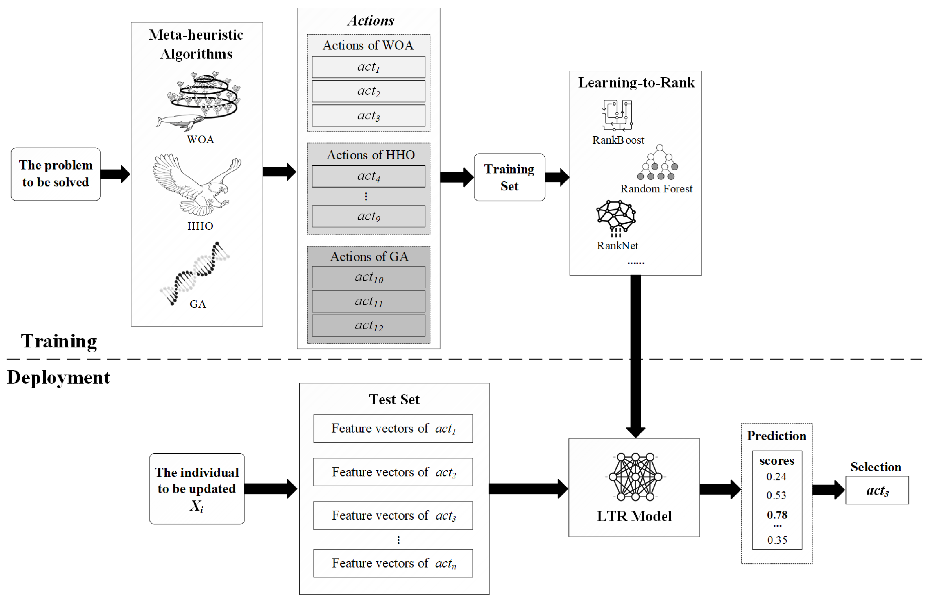
The core concept of the LTR-MHA method is to leverage the LTR framework to extract knowledge from historical execution data of multiple metaheuristic algorithms. The trained prediction model dynamically predicts the scores of candidate update behaviors during the search process, thereby intelligently selecting the update behavior most likely to improve the current solution. The overall methodological flow is illustrated in Figure 1.
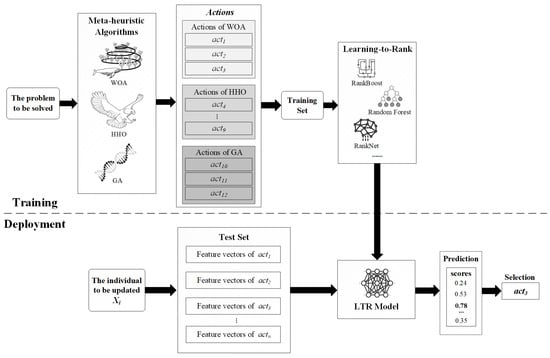
Figure 1.
Overall flowchart of the LTR-MHA.
First, information is extracted from the update behaviors during the solving process of metaheuristic algorithms to construct a feature set and the corresponding label set. Next, a prediction model is trained to learn the relationship between different update behaviors and solution quality, which is used to predict the effectiveness of each candidate update behavior. Once the prediction model is trained, the relevant feature vectors of all candidate behaviors for the search agent to be updated are input into the model. By evaluating the feature vector of the current search agent, the model predicts a corresponding score, which reflects the potential solution quality after applying the given update behavior. Finally, the behavior with the highest predicted score is chosen to update agents.
In this way, the search process of algorithm can be guided more intelligently, avoiding blind exploration and thereby improving convergence speed and solution quality. The innovation of the LTR-MHA lies in applying LTR to learn the ranking of metaheuristic algorithm behaviors, enabling the automated generation of new algorithms. This approach breaks through the fixed search framework of traditional metaheuristic algorithms and offers a novel perspective for tackling optimization tasks. Notably, the primary objective of this study is not to identify the optimal algorithm combination but to verify the feasibility of multi-algorithm integration strategies in boosting the performance of individual algorithms. Based on this objective, three representative classical metaheuristic algorithms (GA, WOA, and HHO) are selected as the subjects of investigation in this work.
4.2. Feature Selection
The training feature set can be represented as a matrix , where each row corresponds to a feature vector, and denotes the feature value of the i-th feature vector at the j-th component. There are three sorts of features: search-dependent, solution-dependent, and instance-dependent [1]. Search-dependent features are relevant to the search procedure, such as overall improvement over the initial solution. Solution-dependent features are linked to the solution encoding scheme. For example, in the TSP, the whole path encoding can be defined explicitly as a feature. Instance-dependent features record the issue instance’s specific properties, such as the number of vehicles and vehicle capacity. It is worth mentioning that when search-dependent or instance-dependent features are used, the knowledge gained can be transferred to other instances of comparable issues or even used to solve different problems. However, solution-dependent features are frequently constrained by unique issues, making it challenging to create generalizable approaches.
Therefore, in this method, search-dependent features are used to construct the feature set. Furthermore, two main coefficient vectors of the WOA, and ; the escape energy E in HHO; and the crossover and mutation rates in the GA are also included as components of the feature set. These parameters help to more comprehensively reflect the performance characteristics of the algorithm under different update behaviors.
Moreover, quantitatively assessing the levels of exploration and exploitation in algorithms remains an open scientific question [34]. To address this issue, a feasible approach is to monitor the diversity of the population during the search process [35,36]. As an important metric, population diversity can provide a certain level of assessment of the exploration and exploitation in metaheuristics. Population diversity describes the extent of dispersion or clustering of search agents during the iterative search process. It can be calculated with the following formula:
where represents the median value of the j-th variable across all individuals in the population, and denotes the value of the j-th variable for the i-th search agent. The total number of agents in the current iteration is given by n, while m represents the number of variables in the potential solution to the optimization problem. The term quantifies the average distance between each individual’s value in the j-th dimension and the median of that dimension, thus representing the diversity of the population along that specific variable. , in turn, is the average of all values across all dimensions, which reflects the overall diversity of the population. It is important to note that population diversity should be recalculated at each iteration. And Table 1 presents the list of feature variables used in this study, along with their definitions.

Table 1.
Feature variables and definitions.
4.3. Feature Extraction and Model Training
The core of the LTR-MHA lies in extracting key features from each iteration update of the metaheuristic algorithms. Specifically, the target problem is solved individually using the selected metaheuristic algorithms (WOA, HHO, and GA). These algorithms optimize solutions through a series of update behaviors, such as shrinking encircling, spiral updating, and random search in the WOA. To systematically represent these diverse update behaviors for the purpose of Learning-to-Rank modeling, each behavior is numerically encoded as a distinct action. Table 2 presents the update behaviors of the three metaheuristic algorithms, along with their corresponding numerical encodings for the convenience of subsequent experiments.
Table 2.
Update behaviors of the metaheuristic algorithms.
Based on the information in Table 2, the action space of the LTR-MHA can be defined as follows:
In continuous function optimization problems, the objective of metaheuristic algorithms is to search for the best solution within the continuous space that minimizes the objective function value. Let the algorithms set be , where the population of algorithm is denoted as , consisting of m search agents (individuals). Each search agent represents a candidate solution. A solution in D-dimensional space is encoded as:
where D represents the dimension, and denotes the j-th variable in the solution vector. Each variable satisfies predefined boundary constraints. By continuously updating the positions of search agents within the population, the algorithm drives the objective function value progressively closer to the global optimum.
At each iteration of the algorithm, the search agent selects one action from multiple candidate update behaviors to update its position and constructs the corresponding feature vector . According to Table 1 and Table 2, suppose the update behavior selected by in the current iteration is , where the value range of is . To ensure that all feature values fall within the range , normalization is applied to each feature individually. The normalization formula for is as follows:
where and represent the upper and lower bounds, which are 12 and 1, respectively. Similarly, and are normalized in the same way. The values of , , and are originally within the range . Meanwhile, and are D-dimensional vectors with each component of in and each component of in , while E is a scalar in . After normalization, these three features are also scaled to . Thus, the feature vector can be expressed as follows:
Here, and denote the j-th component of the coefficient vectors and corresponding to the i-th individual in the population. To convert the vector-valued parameters into scalar features, we compute the the mean value of and as follows: .
It is worth noting that the information from unselected candidate actions is also crucial for model training. Therefore, corresponding feature samples need to be constructed for these actions as well. To prevent any impact on the optimization process, a replica of the current search agent should be created to simulate the updates of other candidate actions and record their feature data. In addition, when constructing the feature set, the core parameter values of other algorithms should be preserved and assigned a value of zero. For example, when executing the WOA algorithm, the parameter E of HHO, as well as the crossover rate and mutation rate of GA, should all be retained in the feature vector but uniformly set to zero. This design ensures the completeness of the feature vector.
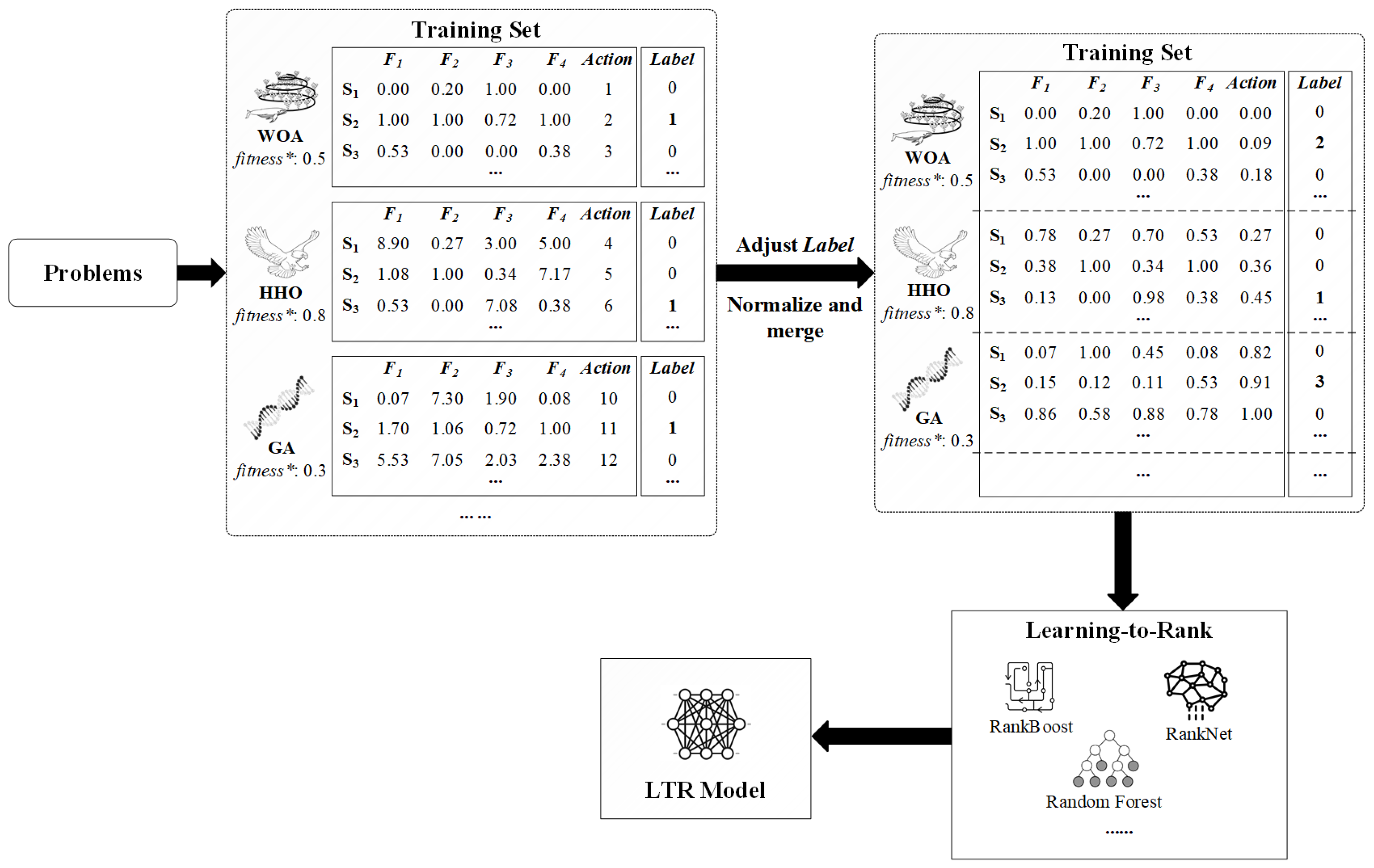
Figure 2 illustrates the flowchart of training set construction and model training. To reduce the complexity of the figure, only a subset of feature vectors (–) is retained as examples.
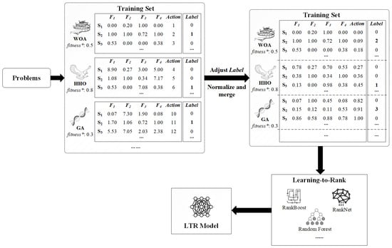
Figure 2.
Flowchart of training set construction and model training of the LTR-MHA.
For the selected action, the is assigned as “1”, while for the unselected candidate actions, the is set to “0”. To assess the performance of three algorithms, we rank their best fitness in descending order (where lower values indicate better solutions) and assign the corresponding ranking numbers as the new values. For example, as shown in Figure 2, if the GA achieves the best fitness values () among the three algorithms, then the for the selected actions within the GA is adjusted from “1” to “3”. Similarly, the for the WOA and HHO are adjusted to “2” and “1”, respectively. This strategy more properly reflects each algorithm’s relative performance during the optimization process, as well as providing more discriminative annotations for predictive model training. After completing the optimization phase of each algorithm, the feature sets corresponding to the optimal solutions provided by the three algorithms are merged to form the training feature set for the prediction model . The detailed implementation of the training set construction for the LTR-MHA is shown in Algorithm 1, with the specific feature extraction and construction process of the metaheuristic algorithm exemplified by the WOA in Algorithm 2.
| Algorithm 1 The procedure of training set construction of LTR-MHA |
|
| Algorithm 2 The procedure of feature extraction and construction of WOA |
|
In Algorithm 1, to ensure fairness in the comparison among the algorithms, a unified initial population is used. Subsequently, the algorithms in the given algorithm set are executed sequentially, and the initial fitness values are calculated (lines 1–4). Within the , the search agents are updated according to the strategies of the metaheuristic algorithms while recording the selected update action and constructing the corresponding feature vector (lines 6–9). The update behaviors of each metaheuristic algorithm (WOA, HHO, GA) are the original, unmodified versions. The specific procedure for feature extraction and construction is illustrated using the WOA as an example, as shown in Algorithm 2. At the same time, the information of unselected candidate actions is equally crucial for model training. Therefore, feature vectors for these actions are also constructed (lines 11–15). In each iteration, the algorithm checks whether the population exceeds the search space boundaries and performs necessary adjustments, followed by recalculating the fitness values of each solution. Whenever a better agent is available, the best agent is updated (lines 19–21). At the end of the algorithm, the best fitness of each algorithm is recorded (line 24). Finally, the algorithms are ranked according to their best fitness values , and their corresponding labels are reassigned based on this ranking. The ranking is in descending order of best fitness, with the resulting position used as the new (lines 26–27). Thus, among the three algorithms, the one with the smallest best fitness value receives the highest label (i.e., ). The feature vectors set and its corresponding labels set together form the training dataset.
During the training stage of the predictive model , the constructed feature set, along with its corresponding label set, is used as the training set. Through supervised learning, the model is able to predict the potential quality of the solutions generated by the update actions performed by the current search agent and produce a prediction score. This score guides the algorithm in making decisions during the search process, steering the exploration toward more promising regions of the solution space. The model is implemented using the standard RandomForestRegressor from scikit-learn, without modification to its core training procedure. The full set of hyperparameter configurations is provided in the experimental settings.
4.4. Algorithm Implementation of LTR-MHA
Once the predictive model is trained, it can be employed to guide the search process. During each iteration, when a search agent requires position updating, the feature vectors for all candidate update actions of the current search agent are first constructed and fed into the predictive model . The model evaluates these feature vectors and outputs a set of predicted scores. Based on these scores, the algorithm selects the candidate action with the highest predicted score for execution. As illustrated in Figure 1, the model predicts that the action corresponds to the solution with the highest predicted score (0.78), indicating that this action is most likely to guide the search process towards the best solution. Therefore, in this iteration, the search agent selects . The implementation of the LTR-MHA is detailed in Algorithm 3.
| Algorithm 3 Pseudocode of LTR-MHA |
|
First, the population of search agents P is initialized, and the fitness value of each search agent is calculated. The best search agent is selected as the initial optimal solution (lines 1–3). Then, within the , for each search agent and candidate action, the feature vectors to be evaluated are constructed. Since this method involves 12 update actions, the feature set to be predicted should contain 12 feature vectors (lines 5–8). These feature vectors are then fed into the predictive model, which outputs a set of predicted scores. The algorithm selects the update action corresponding to the highest predicted score for execution (lines 9–11). Subsequently, the algorithm checks whether any search agent has exceeded the search space boundaries, adjusts their positions accordingly, and recalculates the fitness values of all search agents (lines 13–14). If a better solution is found, the is updated (line 14). After the loop ends, the final optimal solution is returned (line 17).
5. Experiment Evaluation
5.1. Experimental Setup
In this study, the performance of the LTR-MHA algorithm is evaluated using the CEC2017 benchmark function set [25]. These functions fall into four categories: unimodal functions (F1–F3), simple multimodal functions (F4–F10), hybrid functions (F11–F20), and composition functions (F21–F30). However, during the actual experiments, errors occurred when invoking functions F2, F16, F17, F20, and F29. Upon investigation, it was found that these issues were primarily caused by numerical instabilities or boundary calculation anomalies in the implementation of these functions on specific platforms. Such issues include overflows, division by zero, or undefined logarithmic operations resulting from extreme inputs. Additionally, certain functions exhibited compatibility issues during the porting process. To ensure the stability and fairness of the experimental results, these functions were reasonably excluded to prevent technical problems from interfering with the overall evaluation. The range of all functions is , with problem dimensions set to D = 10, 30, 50, and 100. Table 3 includes information about the CEC2017.
Table 3.
CEC2017 test suite.
The objective of the experiments is to confirm the effectiveness of the LTR-MHA method, focusing on three aspects: convergence speed, solution precise, and computing efficiency. The LTR-MHA is compared against individual metaheuristic algorithms, namely the WOA, HHO, and the GA. Under the same algorithmic framework, a comparison is conducted with the Rand-MHA method, which adopts a random update strategy. In the Rand-MHA, the update operation is randomly selected at each position update step, without relying on any learning process, meaning that each update operation has an equal probability of being chosen. Additionally, our approach is compared to two recent improved algorithms, namely the ISGA [8] and RLWOA [13].
In all comparative experiments, the algorithm parameters are uniformly configured to ensure the fairness and reproducibility of the experiments. Specifically, during the training phase, one function from each of the four categories in the CEC2017 benchmark suite is selected to form the training function set. In this study, functions F1, F4, F11, and F21 are chosen as the training set. Therefore, these four functions are excluded from the testing phase to avoid evaluation bias, as they have been used to train the Learning-to-Rank model. This ensures a fair performance comparison on unseen benchmark functions. For each function in the benchmark set, algorithms are each run 15 times, with the population size and iterations set to 30 and 500, respectively. Other settings are summarized in Table 4 for reproducibility.
Table 4.
Parameter configurations for all algorithms used in the experiments.
To further eliminate the influence of initial randomness, all algorithms use the same initial population configuration, ensuring that performance differences arise primarily from the algorithmic mechanisms rather than stochastic factors. Subsequently, the historical information of the optimal solutions is used as training data to train the predictive model based on a Random Forest ranking algorithm. During the testing phase, the trained predictive model is applied to test functions other than F1, F4, F11, and F21. To reduce the effect of randomness on the experimental outcomes, each algorithm is executed independently 15 times.
5.2. Experimental Results and Discussion
Table 5, Table 6 and Table 7 present a comparison of the results between the LTR-MHA and the baseline algorithms, focusing on the mean, standard deviation, and best solution values. The best average value is highlighted in bold. The statistics demonstrate that our proposed method significantly outperforms the others in solving various test functions across different dimensions.
Table 5.
Comparison of unimodal and simple multimodal functions.
Table 6.
Comparison of hybrid functions.
Table 7.
Comparison of composition functions.
Specifically, in solving unimodal and simple multimodal functions (as shown in Table 5), the LTR-MHA consistently achieves the lowest average values across most functions, demonstrating a remarkable advantage. Additionally, the LTR-MHA maintains the lowest or second-lowest standard deviation in nearly all functions and dimensions, indicating a more stable convergence process. In certain cases, such as functions F3, F7, and F9, the GA occasionally attains the lowest average value, suggesting that traditional heuristic algorithms still remain competitive when dealing with relatively simple problem structures. Furthermore, the RLWOA occasionally obtains the best average value among all compared methods, highlighting the effectiveness of parameter adaptation based on reinforcement learning. Overall, the RLWOA ranks directly after the LTR-MHA and Rand-MHA in solution precision. Moreover, although the Rand-MHA performs reasonably well in terms of solution accuracy, its generally higher standard deviations reveal a lack of stability in the algorithm’s performance.
Table 6 shows that the performance gap between algorithms increases when evaluated on hybrid functions. The LTR-MHA achieves the lowest average values on F14 and F18 and secures the best solutions across nearly all dimensions while also maintaining the lowest standard deviations. This demonstrates its ability to obtain high-precision solutions and maintain excellent convergence consistency in high-dimensional search spaces. The GA and Rand-MHA, on the other hand, approach the LTR-MHA’s performance on certain functions. In particular, the Rand-MHA and the GA outperform the LTR-MHA in terms of average performance on F13 and F15. This indicates that the LTR-MHA’s learning model still has room for improvement in terms of stability and accuracy when handling certain complex hybrid structures. By contrast, the performance of the WOA and HHO degrades significantly in high-dimensional environments, with their convergence curves exhibiting considerable fluctuations. The ISGA and RLWOA exhibit comparable results to the baseline methods but do not surpass the LTR-MHA on the tested hybrid functions, indicating limitations when addressing complex hybrid functions.
When tackling the composition functions in the CEC2017 benchmark (Table 7), the LTR-MHA demonstrates a significant advantage across most functions: it consistently achieves the lowest average values (e.g., F22, F23, F24, and F30), as well as the best solutions, while maintaining relatively low standard deviations. The GA performs notably well on certain high-dimensional problems (e.g., F25). The RLWOA obtains the best average value on F28, ranking after the LTR-MHA in overall composition function performance. Although the Rand-MHA approaches the performance of the LTR-MHA in some lower-dimensional scenarios, its results exhibit considerable fluctuations in high-dimensional settings. Overall, the WOA and HHO show relatively poor performance, indicating limited adaptability to complex problems. In summary, the LTR-MHA delivers the best overall performance in composition function optimization, particularly excelling in high-dimensional problems by balancing both accuracy and robustness, while traditional algorithms remain competitive only in specific, simpler cases.
To balance problem complexity with an effective evaluation of algorithmic performance, the convergence speed and runtime analyses are conducted using the 30-dimensional test functions. On one hand, 10-dimensional problems are relatively simple and may not adequately demonstrate the advantages of the algorithm in complex search spaces. On the other hand, 100-dimensional problems can be overly complex, potentially leading to inefficient searches and making algorithm performance highly susceptible to random factors. The 30-dimensional setting, which is widely adopted in current academic research, strikes an appropriate balance between computational cost and evaluation depth, thereby providing a reliable basis for validating the algorithm’s performance [37,38].
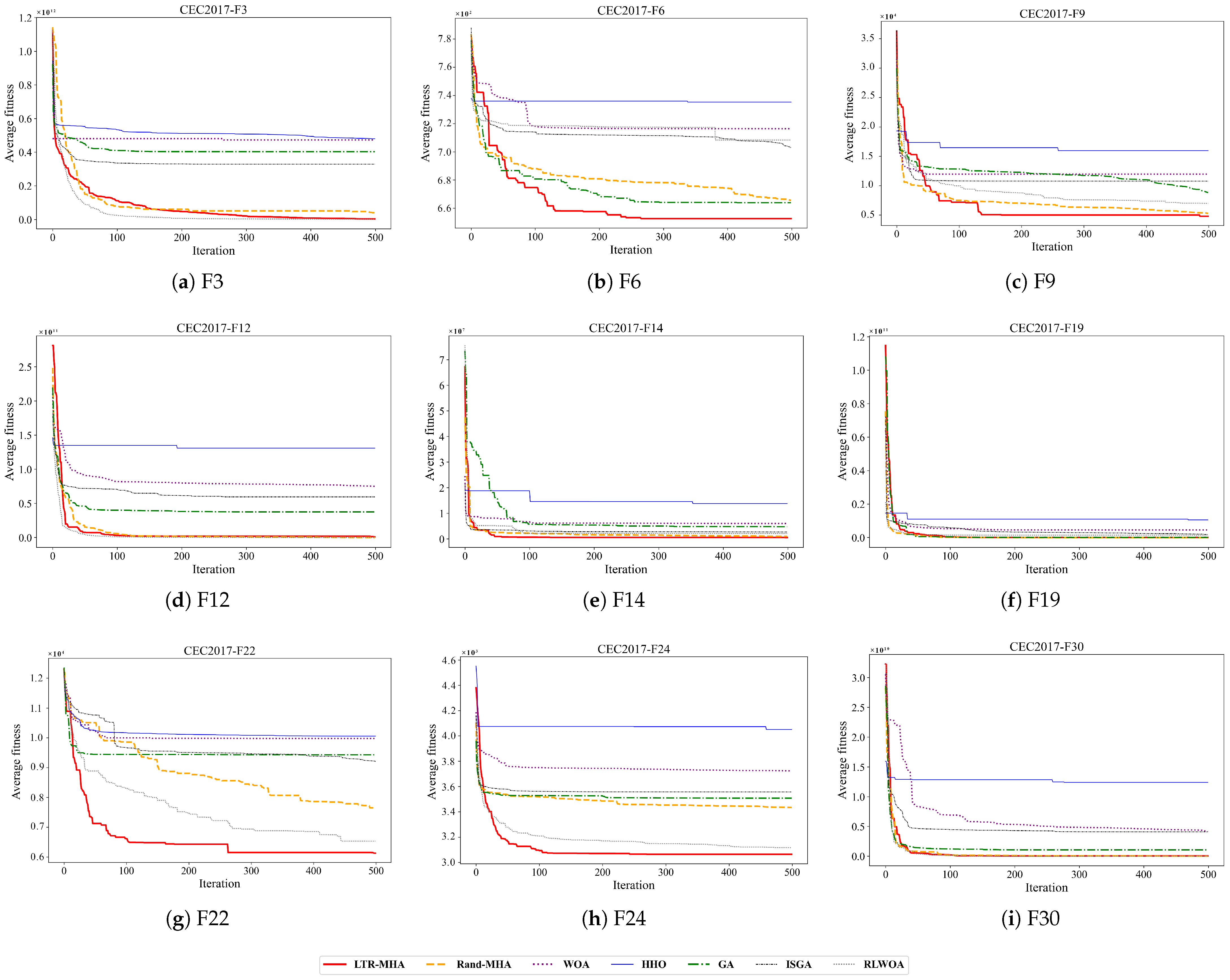
Figure 3 shows the average fitness convergence curves of five algorithms on nine typical functions (F3, F6, F9, F12, F14, F19, F22, F24, and F30) from the CEC2017 benchmark, with a dimensional setting of . Overall, the proposed LTR-MHA demonstrates the best final fitness values on most test functions, with its advantages being particularly evident on multimodal and composition functions (e.g., F6, F22, and F24), approaching the optimal region within just 100 iterations, whereas the other algorithms generally converge more slowly and are more prone to local optima. Although the Rand-MHA, with its random update strategy, surpasses traditional metaheuristic algorithms on certain functions (e.g., F3, F9, F14, and F24), its overall performance still lags behind the LTR-MHA and exhibits greater variability. Among the three conventional algorithms, the GA performs the best. The ISGA yields convergence behavior similar to the GA across most functions. The RLWOA converges rapidly on a majority of the tested functions, achieving final fitness values that are comparable to or only marginally lower than those of the LTR-MHA. HHO, despite occasionally achieving a rapid decline in the early iterations, suffers from premature convergence and stagnates in the later stages, resulting in noticeably poorer final solutions. These findings demonstrate that the multi-strategy fusion update mechanism learned by the LTR-MHA enables stable and efficient optimization across various types of complex search spaces.
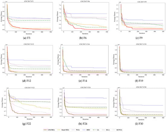
Figure 3.
Convergence curves for the functions with D = 30.
Table 8 presents the average runtime of the five algorithms on the CEC2017 test functions. The results indicate that the WOA consistently exhibits the lowest computational overhead across all test functions, with an average runtime ranging from 0.4 to 0.96 s. The GA follows closely, requiring approximately 0.7 to 1.5 s. Due to its more complex internal search strategies, HHO incurs a longer runtime of 1.4 to 8.9 s. The Rand-MHA, which involves randomly selecting and executing multiple update operations in each iteration, experiences a further increase in average runtime. The ISGA takes about 4 to 7 s per run, which reflects its additional clustering and adaptive migration techniques. The RLWOA holds the highest overhead among compared methods, with runtimes ranging from 56 to 60 s due to its online reinforcement learning-based parameter adjustment. The LTR-MHA, requiring feature generation and online prediction via the model at each iteration, introduces additional computational complexity, resulting in the longest runtime among the compared algorithms. This difference arises from the algorithmic design of the LTR-MHA. In each iteration, for every individual in the population, the LTR-MHA constructs candidate update strategies. Each candidate is represented by a feature vector composed of 10 components (as shown in Equation (19)). These m feature vectors are then passed into the trained predictive model to compute scores and select the most promising strategy. As a result, the per-iteration time complexity of the LTR-MHA is approximately , where n is the population size, is the feature dimension, is the model’s prediction time, and D is the problem dimension. This is significantly higher than other metaheuristics that apply a single, fixed rule per individual per iteration. In conclusion, while the LTR-MHA clearly outperforms in convergence speed and solution precision, its increased computational cost requires a trade-off with time efficiency in practical applications.
Table 8.
Average runtime comparison of LTR-MHA and baseline algorithms (in seconds).
Notably, the development time of automated methods and manually designed approaches is generally difficult to compare directly, as such information is typically not disclosed in published studies. Furthermore, although the proposed algorithm incurs additional computational time in both the training and testing steps, the primary goal of this research is not to discover the optimal approach but rather to explore an approach capable of automatically generating highly generalizable and state-of-the-art search strategies. In the long term, this additional computational overhead is justified by the ability to efficiently solve a broad range of problem instances.
The Wilcoxon rank-sum test was used at a significance level of 0.05 to determine whether the LTR-MHA’s optimization results outperformed the compared algorithms significantly. Table 9 presents the statistical analysis results of the LTR-MHA against the other algorithms under the 30-dimension setting. In the table, the symbols ‘+’, ‘=’, and ‘−’ demonstrate that the LTR-MHA performs significantly better than, similarly to, and significantly worse than the compared algorithm. As shown in Table 9, the LTR-MHA predominantly achieves the ‘+’ symbol across most cases, indicating that its performance on the CEC2017 benchmark optimization tasks is significantly superior to that of the other algorithms.
Table 9.
Results of Wilcoxon rank-sum test.
In summary, the LTR-MHA shows significant advantages in solution precision, convergence speed, and statistical significance. Across tests on unimodal, simple multimodal, hybrid, and composite functions, the LTR-MHA consistently yields the lowest average fitness values in most scenarios while maintaining the lowest or second-lowest standard deviations. Moreover, the LTR-MHA is able to rapidly approach the optimal regions, particularly in simple multimodal and composite functions. Although the model prediction process leads to longer runtimes, this additional computational cost is offset in the long term by the algorithm’s ability to efficiently solve a wide range of problem instances. In contrast, traditional metaheuristic algorithms exhibit acceptable performance in specific functions or lower-dimensional problems but suffer significant degradation in high-dimensional, complex environments. Therefore, by leveraging a multi-strategy fusion mechanism, the LTR-MHA effectively addresses complex optimization problems, though the trade-off between computational cost and performance should be carefully considered in practical applications based on specific problem requirements.
6. Conclusions
To address the limitations of flexibility and adaptability in traditional metaheuristic algorithms when dealing with diverse optimization problems, as well as their tendency to get trapped in local optima, this paper proposes the LTR-MHA, an automated algorithm generation method based on Learning to Rank. This approach analyzes the historical search processes of the GA, WOA, and HHO to extract key features, including the iteration stage, core algorithm parameters, and diversity metrics, for constructing the training dataset. A predictive model is then trained using the Random Forest algorithm. During the optimization process, the LTR-MHA dynamically evaluates the potential benefit scores of candidate update actions and intelligently selects the optimal update strategy. This allows the method to significantly improve search efficiency, minimize premature convergence, and improve the quality of the solution.
Experimental validation via the CEC2017 benchmark test suite demonstrates that the LTR-MHA exhibits clear advantages across unimodal, simple multimodal, hybrid, and composition function tests. Compared with single algorithms and random combination strategies, the LTR-MHA consistently yields the lowest average and the best fitness values in nearly all test scenarios while maintaining strong stability. In particular, for multimodal and high-dimensional problems, the LTR-MHA effectively accelerates convergence through its multi-strategy integration mechanism. Although the model prediction introduces additional computational overhead, considering the overall balance between algorithm performance and computational cost, the LTR-MHA still delivers a favorable cost/performance ratio in practical applications.
Future research will further explore the search characteristics of different metaheuristic algorithms, investigate the optimal number of algorithm combinations, and develop more rational combination strategies. Additionally, we will be made to incorporate other artificial intelligence techniques or optimization algorithms to improve model prediction efficiency and reduce computational overhead, ultimately achieving a more efficient real-time algorithm selection strategy. The LTR-MHA methodology will next be compared to existing state-of-the-art approaches and applied to more challenging circumstances to ensure its generalizability and practical relevance.
Author Contributions
X.X.: Data Curation, Software, Writing—Original Draft. T.S.: Methodology, Conceptualization, Investigation, Writing—Review and Editing. J.X.: Resources, Validation. All authors have read and agreed to the published version of the manuscript.
Funding
This research was funded by the Zhejiang Provincial Natural Science Foundation of China (Grant No. LY22F020019), the Public-Welfare Technology Application Research of Zhejiang Province in China (Grant No. LGG22F020032), the Zhejiang Science and Technology Plan Project (Grant No. 61972359), and the National Natural Science Foundation of China (Grant No. 62132014).
Data Availability Statement
Data will be made available on request.
Conflicts of Interest
The authors declare no conflicts of interest.
References
- Yi, W.; Qu, R.; Jiao, L.; Niu, B. Automated design of metaheuristics using reinforcement learning within a novel general search framework. IEEE Trans. Evol. Comput. 2022, 27, 1072–1084. [Google Scholar] [CrossRef]
- Yi, W.; Qu, R. Automated design of search algorithms based on reinforcement learning. Inf. Sci. 2023, 649, 119639. [Google Scholar] [CrossRef]
- Wolpert, D.H.; Macready, W.G. No free lunch theorems for optimization. IEEE Trans. Evol. Comput. 1997, 1, 67–82. [Google Scholar] [CrossRef]
- Kareem, S.W.; Ali, K.W.; Askar, S.; Xoshaba, F.S.; Hawezi, R. Metaheuristic algorithms in optimization and its application: A review. JAREE 2022, 6, 7–12. [Google Scholar] [CrossRef]
- Wang, S.; Lo, D.; Jiang, L.; Lau, H.C. Search-based fault localization. In Proceedings of the 26th IEEE/ACM International Conference on Automated Software Engineering, Lawrence, KS, USA, 6–10 November 2011; pp. 556–559. [Google Scholar]
- Gavvala, S.K.; Jatoth, C.; Gangadharan, G.R.; Buyya, R. QoS-aware cloud service composition using eagle strategy. Future Gener. Comput. Syst. 2019, 90, 273–290. [Google Scholar] [CrossRef]
- Abraham, O.L.; Ngadi, M.A. A comprehensive review of dwarf mongoose optimization algorithm with emerging trends and future research directions. Decis. Anal. J. 2025, 14, 100551. [Google Scholar] [CrossRef]
- Bian, H.; Li, C.; Liu, Y.; Tong, Y.; Bing, S.; Chen, J.; Zhang, Z. Improved snow geese algorithm for engineering applications and clustering optimization. Sci. Rep. 2025, 15, 4506. [Google Scholar] [CrossRef]
- Ryser-Welch, P.; Miller, J.F. A review of hyper-heuristic frameworks. In Proceedings of the Evo20 Workshop, AISB, London, UK, 1–4 April 2014. [Google Scholar]
- Talbi, E.-G. Machine learning into metaheuristics: A survey and taxonomy. ACM Comput. Surv. 2021, 54, 1–32. [Google Scholar] [CrossRef]
- Becerra-Rozas, M.; Lemus-Romani, J.; Crawford, B.; Soto, R.; Cisternas-Caneo, F.; Embry, A.T.; Molina, M.A.; Tapia, D.; Castillo, M.; Misra, S. Reinforcement learning based whale optimizer. In Proceedings of the International Conference on Computational Science and Its Applications, Cagliari, Italy, 13–16 September 2021; pp. 205–219. [Google Scholar]
- Li, K.; Lai, G.; Yao, X. Interactive evolutionary multiobjective optimization via learning to rank. IEEE Trans. Evol. Comput. 2023, 27, 749–763. [Google Scholar] [CrossRef]
- Seyyedabbasi, A. A reinforcement learning-based metaheuristic algorithm for solving global optimization problems. Adv. Eng. Softw. 2023, 178, 103411. [Google Scholar] [CrossRef]
- Talbi, E.-G. A unified taxonomy of hybrid metaheuristics with mathematical programming, constraint programming and machine learning. In Hybrid Metaheuristics; Springer: Berlin/Heidelberg, Germany, 2013; pp. 3–76. [Google Scholar]
- Jin, H.; Yao, X.; Chen, Y. Correlation-aware QoS modeling and manufacturing cloud service composition. J. Intell. Manuf. 2017, 28, 1947–1960. [Google Scholar] [CrossRef]
- Jin, H.; Lv, S.; Yang, Z.; Liu, Y. Eagle strategy using uniform mutation and modified whale optimization algorithm for QoS-aware cloud service composition. Appl. Soft Comput. 2022, 114, 108053. [Google Scholar] [CrossRef]
- Lu, Y.; Yi, C.; Li, J.; Li, W. An Enhanced Opposition-Based Golden-Sine Whale Optimization Algorithm. In Proceedings of the International Conference on Cognitive Computing, Shenzhen, China, 17–18 December 2023; pp. 60–74. [Google Scholar]
- Semenikhin, S.V.; Denisova, L.A. Learning to rank based on modified genetic algorithm. In Proceedings of the 2016 Dynamics of Systems, Mechanisms and Machines (Dynamics), Omsk, Russia, 15–17 November 2016; pp. 1–5. [Google Scholar]
- Oliva, D.; Martins, M.S.R.; Hinojosa, S.; Elaziz, M.A.; dos Santos, P.V.; da Cruz, G.; Mousavirad, S.J. A hyper-heuristic guided by a probabilistic graphical model for single-objective real-parameter optimization. Int. J. Mach. Learn. Cybern. 2022, 13, 3743–3772. [Google Scholar] [CrossRef]
- Kallestad, J.; Hasibi, R.; Hemmati, A.; Sørensen, K. A general deep reinforcement learning hyperheuristic framework for solving combinatorial optimization problems. Eur. J. Oper. Res. 2023, 309, 446–468. [Google Scholar] [CrossRef]
- Hsieh, F.-S. Creating Effective Self-Adaptive Differential Evolution Algorithms to Solve the Discount-Guaranteed Ridesharing Problem Based on a Saying. Appl. Sci. 2025, 15, 3144. [Google Scholar] [CrossRef]
- Hsieh, F.-S. Applying “Two Heads Are Better Than One” Human Intelligence to Develop Self-Adaptive Algorithms for Ridesharing Recommendation Systems. Electronics 2024, 13, 2241. [Google Scholar] [CrossRef]
- Xu, T.; Chen, C. DBO-AWOA: An Adaptive Whale Optimization Algorithm for Global Optimization and UAV 3D Path Planning. Sensors 2025, 25, 2336. [Google Scholar] [CrossRef]
- Norat, R.; Wu, A.S.; Liu, X. Genetic Algorithms with Self-Adaptation for Predictive Classification of Medicare Standardized Payments for Physical Therapists. Expert Syst. Appl. 2023, 218, 119529. [Google Scholar] [CrossRef]
- Wu, G.; Mallipeddi, R.; Suganthan, P.N. Problem Definitions and Evaluation Criteria for the CEC 2017 Competition on Constrained Real-Parameter Optimization; Technical Report; Nanyang Technological University: Singapore, 2017; Available online: https://www.researchgate.net/publication/317228117_Problem_Definitions_and_Evaluation_Criteria_for_the_CEC_2017_Competition_and_Special_Session_on_Constrained_Single_Objective_Real-Parameter_Optimization (accessed on 26 May 2025).
- Mirjalili, S.; Lewis, A. The whale optimization algorithm. Adv. Eng. Softw. 2016, 95, 51–67. [Google Scholar] [CrossRef]
- Heidari, A.A.; Mirjalili, S.; Faris, H.; Aljarah, I.; Mafarja, M.; Chen, H. Harris hawks optimization: Algorithm and applications. Future Gener. Comput. Syst. 2019, 97, 849–872. [Google Scholar] [CrossRef]
- Holland, J.H. Genetic algorithms. Sci. Am. 1992, 267, 66–73. [Google Scholar] [CrossRef]
- Burges, C.; Shaked, T.; Renshaw, E.; Lazier, A.; Deeds, M.; Hamilton, N.; Hullender, G. Learning to rank using gradient descent. In Proceedings of the 22nd International Conference on Machine Learning, Bonn, Germany, 7–11 August 2005; pp. 89–96. [Google Scholar]
- Li, P.; Wu, Q.; Burges, C. McRank: Learning-to-rank using multiple classification and gradient boosting. In Proceedings of the 20th International Conference on Neural Information Processing Systems, Vancouver, BC, Canada, 3–6 December 2007; p. 904. [Google Scholar]
- Crammer, K.; Singer, Y. Pranking with ranking. In Advances in Neural Information Processing Systems; MIT Press: Cambridge, MA, USA, 2001; Volume 14. [Google Scholar]
- Freund, Y.; Iyer, R.; Schapire, R.E.; Singer, Y. An efficient boosting algorithm for combining preferences. J. Mach. Learn. Res. 2003, 4, 933–969. [Google Scholar]
- Cao, Z.; Qin, T.; Liu, T.-Y.; Tsai, M.-F.; Li, H. Learning to rank: From pairwise approach to listwise approach. In Proceedings of the 24th International Conference on Machine Learning, Corvallis, OR, USA, 20–24 June 2007; pp. 129–136. [Google Scholar]
- Morales-Castañeda, B.; Zaldivar, D.; Cuevas, E.; Fausto, F.; Rodríguez, A. A better balance in metaheuristic algorithms: Does it exist? Swarm Evol. Comput. 2020, 54, 100671. [Google Scholar] [CrossRef]
- Fausto, F.; Reyna-Orta, A.; Cuevas, E.; Andrade, Á.G.; Perez-Cisneros, M. From ants to whales: Metaheuristics for all tastes. Artif. Intell. Rev. 2020, 53, 753–810. [Google Scholar] [CrossRef]
- Kriegel, H.-P.; Schubert, E.; Zimek, A. The (black) art of runtime evaluation: Are we comparing algorithms or implementations? Knowl. Inf. Syst. 2017, 52, 341–378. [Google Scholar] [CrossRef]
- Plevris, V.; Solorzano, G. A collection of 30 multidimensional functions for global optimization benchmarking. Data 2022, 7, 46. [Google Scholar] [CrossRef]
- Piotrowski, A.P.; Napiorkowski, J.J.; Piotrowska, A.E. Choice of benchmark optimization problems does matter. Swarm Evol. Comput. 2023, 83, 101378. [Google Scholar] [CrossRef]
Disclaimer/Publisher’s Note: The statements, opinions and data contained in all publications are solely those of the individual author(s) and contributor(s) and not of MDPI and/or the editor(s). MDPI and/or the editor(s) disclaim responsibility for any injury to people or property resulting from any ideas, methods, instructions or products referred to in the content. |
© 2025 by the authors. Licensee MDPI, Basel, Switzerland. This article is an open access article distributed under the terms and conditions of the Creative Commons Attribution (CC BY) license (https://creativecommons.org/licenses/by/4.0/).