Phymastichus–Hypothenemus Algorithm for Minimizing and Determining the Number of Pinned Nodes in Pinning Control of Complex Networks

Abstract

Pinning control is a key strategy for stabilizing complex networks through a limited set of nodes. However, determining the optimal number and location of pinned nodes under dynamic and structural constraints remains a computational challenge. This work proposes an improved version of the Phymastichus–Hypothenemus Algorithm—Minimized and Determinated (PHA-MD) to solve multi-constraint, hybrid optimization problems in pinning control without requiring a predefined number of control nodes. Inspired by the parasitic behavior of Phymastichus coffea on Hypothenemus hampei, the algorithm models each agent as a parasitoid capable of propagating influence across a network, inheriting node importance and dynamically expanding search dimensions through its “offspring.” Unlike its original formulation, PHA-MD integrates variable-length encoding and V-stability assessment to autonomously identify a minimal yet effective pinning set. The method was evaluated on benchmark network topologies and compared against state-of-the-art heuristic algorithms. The results show that PHA-MD consistently achieves asymptotic stability using fewer pinned nodes while maintaining energy efficiency and convergence robustness. These findings highlight the potential of biologically inspired, dimension-adaptive algorithms in solving high-dimensional, combinatorial control problems in complex dynamical systems.

1. Introduction

Recently, research on the analysis and control of complex networks has advanced rapidly [1]. The presence of complex networks in nature and society has sparked significant interest in this field [2], as they are integral to various systems in our daily lives [3]. For instance, the organization and function of a cell result from complex interactions between genes, proteins, and other molecules [4]; the brain comprises a vast network of interconnected neurons [5]; social systems can be represented by graphs illustrating interactions among individuals [6]; ecosystems consist of species whose interdependencies can be mapped into food webs [7]; and large networked infrastructures, such as power grids and transportation networks, can be represented by graphs describing interactions among components [8,9].

In complex networks, a key challenge is ensuring control and stability while minimizing resource consumption. This requires selecting a subset of nodes, known as pinning nodes, to control the entire network. Pinning control achieves global stabilization by intervening in these selected nodes. The optimal selection of these nodes is crucial, with various centrality metrics, like Degree Centrality [10], Betweenness Centrality [11], and Closeness Centrality [12], proposed in the literature. These metrics offer different advantages depending on the network’s structure and dynamics [3,13,14].

Recent advances in complex network control have led to more sophisticated algorithms designed to handle the growing complexity of modern networks. Techniques such as adaptive control [15], robust control [16], and sliding mode control [17] have been developed to improve stability and robustness under various uncertainties. However, these methods often struggle with the optimal selection of pinning nodes, especially in large networks with vast combinations of nodes.

Existing methods are limited by their reliance on fixed-dimension approaches and their difficulty adapting to dynamic network environments. These algorithms often require prior knowledge of the network’s structure, which may not always be available, and can become computationally expensive as the network grows, making them impractical for real-time use.

The PHA-MD algorithm proposed in this work addresses these limitations by offering a novel approach to pinning control. Inspired by the parasitic relationship between the Phymastichus coffea wasp and the Hypothenemus hampei coffee borer, PHA-MD prioritizes the network’s asymptotic stability while optimizing pinning node selection. Unlike its predecessor [18,19], PHA-MD autonomously determines the number of pinning nodes, avoiding the issues associated with fixed-dimension algorithms. This innovation allows PHA-MD to dynamically adapt to network changes, ensuring stability even in complex scenarios.

PHA-MD also leverages the V-stability tool [20] to ensure stability during optimization. Comparative simulations demonstrate PHA-MD’s superior performance compared to several heuristic optimization algorithms, particularly in achieving network stability with fewer pinned nodes and efficient energy use.

The performance of PHA-MD is compared with other heuristic optimization algorithms, such as Ant Lion Optimizer (ALO) [21], Teaching–Learning-Based Optimization (TLBO) [22], Grey Wolf Optimizer (GWO) [23], Animal Migration Optimization (AMO) [24], Particle Swarm Optimization (PSO) [25], Artificial Bee Colony (ABC) [26], Gaining–Sharing Knowledge Based Algorithm (GSK) [27], Biogeography-Based Optimization (BBO) [28], Whale Optimization Algorithm (WOA) [29], Ant Colony Optimization (ACO) [30], Osprey Optimization Algorithm (OOA) [31], Mayfly Algorithm (MA) [32], Archimedes Optimization Algorithm (AOA) [33], Coronavirus Herd Immunity Optimizer (CHIO) [34], and Driving Training-Based Optimization (DTBO) [35].

These algorithms were selected for several reasons. They represent a wide range of optimization techniques, from bio-inspired methods like ALO [21] and PSO [25] to recent innovations such as CHIO [34] and OOA [31]. This diversity allows for a comprehensive comparison across different strategies. Many of these algorithms have shown high performance in solving complex optimization problems, making them robust benchmarks for evaluating PHA-MD. Their popularity in the research community ensures that the comparison results are relevant and easily interpretable.

The selected algorithms also cover different optimization mechanisms, including swarm intelligence (PSO, WOA [29]), natural evolution (Genetic Algorithm (GA) [36]), intensive local search (GWO [23]), and reinforcement learning (Q-Learning based algorithms [37]). Comparing PHA-MD with these approaches helps its competitiveness with the latest developments in heuristic optimization.

In summary, the selection of these algorithms provides a rigorous benchmarking framework, allowing for a thorough assessment of PHA-MD’s capabilities, particularly in solving the permutation problem in node selection and ensuring the network’s asymptotic stability. Additionally, PHA-MD’s ability to handle multi-constraint optimization problems makes it versatile and effective in various applications.

The rest of this paper is organized as follows. Section 2 provides an overview of complex network pinning control, detailing the V-stability tool and other essential mathematical preliminaries. This section also defines the optimization problem, focusing on minimizing the energy consumed by control actions at the pinning nodes and the number of pinning nodes required for network stability. In Section 3, the biological foundation of the PHA-MD algorithm is described, highlighting its unique characteristics and mechanisms. Section 4 presents a comprehensive simulation study of the proposed PHA-MD algorithm across various complex network topologies, including a detailed comparison with other heuristic optimization algorithms. Finally, Section 5 discusses the conclusions and potential future directions of the research.

2. Problem Statement

The optimization problem in complex networks is formulated to achieve two primary objectives:

(i)

Minimizing the energy consumed by the control actions at the pinning nodes: this objective focuses on reducing the overall energy required to stabilize the network through targeted interventions at selected nodes.

(ii)

Minimizing the number of pinning nodes required to achieve network stability: this objective aims to reduce the number of nodes that need to be pinned to maintain the stability of the entire network, thereby optimizing resource usage.

These objectives define the optimization problem as follows. Let $M\equiv Q(\Theta ,G,K)$ denote the closed-loop matrix built from the node passivity degrees $\Theta$, the coupling matrix G, and the diagonal gain matrix K; let $\lambda \left\{·\right\}$ denote the spectrum (set of eigenvalues); and let $R_e\left\{·\right\}$ denote the real-part operator applied to those eigenvalues. Then

$$\begin{array}{cc}\mathrm{minimize}\hfill & \left\{f\right(\mathcal{U}),\mathrm{card}(\mathcal{U}\left)\right\}\hfill \\ \mathrm{subject}\mathrm{to}\hfill & \mathcal{U}\subseteq \{1,\dots ,N_n\},\hfill \\ \hfill & max\left\{R_e\left\{\lambda \left\{M\right\}\right\}\right\}<0,\hfill \end{array}$$

(1)

where $\mathcal{U}$ is the index set of pinning nodes and $\mathrm{card}\left(\mathcal{U}\right)$ is its cardinality. The control law for node $n_i$ is ${\mathbf{u}}_i=-k_i{\mathbf{x}}_i$, with ${\mathbf{x}}_i={(x_{i,1},x_{i,2},\dots ,x_{i,N_s})}^T\in {\mathbb{R}}^{N_s}$ and $k_i\ge 0$ the i-th diagonal entry of K, defined as

$$K_{i,i}=\left\{\begin{array}{cc}{k}_i,\hfill & i\in \mathcal{U},\hfill \\ 0,\hfill & i\notin \mathcal{U}.\hfill \end{array}\right.$$

The inequality $max{R}_e\left\{\lambda \left\{M\right\}\right\}<0$ expresses exponential stability.

Specifically, the optimization problem involves the construction of the control gain matrix K. The goal is to find the optimal set of pinning nodes that achieves efficient network control. In this context, the construction of the control gain matrix K is crucial. The matrix K determines the effectiveness of the pinning control strategy, directly impacting the stability and efficiency of the network. Ensuring an optimal configuration of K is essential for achieving network stability with minimal resource consumption. Thus, the following describes the relevance of the matrix K in the pinning control of complex networks, and its impact on the stability of the network.

Consider the following Network (2) of $N_n$ nodes with linear diffusive couplings and an $N_s$-dimensional dynamical system [38]:

$${\dot{\mathbf{x}}}_i=f_i\left({\mathbf{x}}_i\right)+\sum _{\begin{array}{c}j=1,j\ne i\end{array}}^{N_n}{c}_{ij}{a}_{ij}\Gamma \left({\mathbf{x}}_j-{\mathbf{x}}_i\right),$$

(2)

where $f_i:{\mathbb{R}}^{N_s}\to {\mathbb{R}}^{N_s}$ denotes the self-dynamics of node $n_i$, i.e., the intrinsic vector field that governs its evolution in isolation (all couplings and controls set to zero). The constants $c_{ij}$ are the coupling strengths between $n_i$ and $n_j$, $\Gamma \in {\mathbb{R}}^{N_s\times N_s}$ specifies how state components are coupled for each connected pair $({\mathbf{x}}_j,{\mathbf{x}}_i)$, and the connection matrix $A=\left[a_{ij}\right]\in {\mathbb{R}}^{N_n\times N_n}$ encodes the network topology: if there is a connection between $n_i$ and $n_j$ for $i\ne j$, then $a_{ij}=a_{ji}=1$; otherwise $a_{ij}=a_{ji}=0$ for $i\ne j$. The diagonal elements are defined by $a_{ii}=-{\sum }_{\begin{array}{c}j=1\\ j\ne i\end{array}}^{N_n}-d_i$, where $d_i$ is the degree of node $n_i$. A small subset of nodes in the network is subjected to local feedback as part of the pinning control, and these are called pinning nodes [39]. Assuming the diffusive condition

$$c_{ii}{a}_{ii}+\sum _{\begin{array}{c}j=1\\ j\ne i\end{array}}^{N_n}{c}_{ij}{a}_{ij}=0,i=1,2,\dots ,N_n,$$

(3)

Network (2) can be rewritten in a compact controlled form as

$${\dot{\mathbf{x}}}_i=f_i\left({\mathbf{x}}_i\right)+\sum _{j=1}^{N_n}{c}_{ij}{a}_{ij}\Gamma {\mathbf{x}}_j+B_i{\mathbf{u}}_i,$$

(4)

where $B_i\in {\mathbb{R}}^{N_s\times N_s}$ is the input (actuation) matrix that maps the control vector ${\mathbf{u}}_i\in {\mathbb{R}}^{N_s}$ into the state derivatives of node $n_i$. In the context of pinning control, $B_i$ specifies which state components are directly actuated (full or partial channels). Typical choices are $B_i=I_{N_s}$ (full–state actuation) or $B_i=\mathrm{diag}\left(b_i\right)$ with $b_i\in {\{0,1\}}^{N_s}$ (selected coordinates), where $I_{N_s}$ denotes the $N_s\times N_s$ identity matrix (ones on the diagonal and zeros elsewhere). Unless otherwise stated, we adopt $B_i=I_{N_s}$ in the simulations.

The control input is defined nodewise as

$${\mathbf{u}}_i\left({\mathbf{x}}_i\right)=\left\{\begin{array}{cc}-k_i{\mathbf{x}}_i,\hfill & i\in \mathcal{U},\hfill \\ 0,\hfill & i\notin \mathcal{U},\hfill \end{array}\right.$$

(5)

where $\mathcal{U}$ is the set of pinning nodes with $1\le \mathrm{card}\left(\mathcal{U}\right)\le N_n$ [40]. Hence, the self-dynamics of the controlled nodes becomes

$${\dot{\mathbf{x}}}_i=f_i\left({\mathbf{x}}_i\right)-k_i{B}_i{\mathbf{x}}_i,i\in \mathcal{U}.$$

(6)

To demonstrate network stability and to calculate the lower bound $N_{{\lambda }^{+}}$ for the number of pinned nodes, consider a continuously differentiable Lyapunov function $V\left({\mathbf{x}}_i\right):D\subseteq {\mathbb{R}}^{N_s}\mapsto {\mathbb{R}}_{+}$, satisfying $V\left(\overline{\mathbf{x}}\right)=0$ with $\overline{\mathbf{x}}\in D$, such that for the self-dynamics (6), there is a scalar ${\theta }_i$ and $k_i$ guaranteeing

$$\begin{array}{cc}{\displaystyle \frac{\partial V\left({\mathbf{x}}_i\right)}{\partial {\mathbf{x}}_i}}(f_i\left({\mathbf{x}}_i\right)-k_{i}B{\mathbf{x}}_i+{\theta }_i\Gamma {\mathbf{x}}_i+k_i\Gamma {\mathbf{x}}_i)<0\hfill & \\ & \hfill \forall {\mathbf{x}}_i\in D_i\subseteq D,{\mathbf{x}}_i\ne 0,\end{array}$$

(7)

where

$${\displaystyle D_i=\{{\mathbf{x}}_i:\parallel {\mathbf{x}}_i-{\overline{\mathbf{x}}}_i\parallel <\alpha \},\alpha >0,D=\bigcup _{i=1}^{N_n}{D}_i,}$$

and ${\theta }_i$ is the passivity degree of $f\left({\mathbf{x}}_i\right)$. Then, to determine whether Network (4) is synchronized at the equilibrium point $\overline{\mathbf{X}}={({\overline{\mathbf{x}}}_1^T,\dots ,{\overline{\mathbf{x}}}_{N_n}^T)}^T$, such that

$${\mathbf{x}}_1\left(t\right)={\mathbf{x}}_2\left(t\right)=\dots ={\mathbf{x}}_{N_n}\left(t\right)\to \overline{\mathbf{x}}\mathrm{as}t\to \infty ,$$

let us consider

$$V_N\left(\mathbf{X}\right)=\sum _{i=1}^{N_n}{\displaystyle \frac{1}{2}}{\mathbf{x}}_i^T\mathbf{P}{\mathbf{x}}_i,\mathbf{P}={\mathbf{P}}^T>0,$$

(8)

for the controlled Network (4); then

$$\begin{array}{cc}\hfill {\dot{V}}_N\left(\mathbf{X}\right)& =\sum _{i=1}^{N_n}{\mathbf{x}}_i^T\mathbf{P}\left(f_i\left({\mathbf{x}}_i\right)+\sum _{j=1}^{N_n}{c}_{ij}{a}_{ij}\Gamma {\mathbf{x}}_j-k_{i}B{\mathbf{x}}_i\right)\hfill \\ \hfill {\dot{V}}_N\left(\mathbf{X}\right)& <\sum _{i=1}^{N_n}{\mathbf{x}}_i^T\mathbf{P}\left({\theta }_i\Gamma {\mathbf{x}}_i+\sum _{j=1}^{N_n}{c}_{ij}{a}_{ij}\Gamma {\mathbf{x}}_j+k_i\Gamma {\mathbf{x}}_i\right)\hfill \end{array}$$

(9)

or, using the Kronecker product,

$${\dot{V}}_N\left(\mathbf{X}\right)<{\mathbf{X}}^T(-\Theta +G-K)\otimes \mathbf{P}\Gamma \mathbf{X},$$

(10)

where $c_{ij}{a}_{ij}$ are the entries of $G\in {\mathbb{R}}^{N_n\times N_n}$, $\Theta =$$\mathrm{diag}({\theta }_1$, ${\theta }_2$, …, ${\theta }_{N_n})$, $K=\mathrm{diag}(k_1,k_2,\dots ,$$k_{N_n})$, and $\mathbf{P}\Gamma \ge 0$. Then, according to [20], Network (2) is locally asymptotically stable around its equilibrium point if the closed-loop characteristic matrix

$$Q=-\Theta +G-K$$

(11)

is negative definite; then, the number of pinned nodes cannot be less than the number of positive eigenvalues $N_{{\lambda }^{+}}$ with $K={\left[0\right]}^{N_n\times N_n}$, such that, $\mathrm{card}\left(\mathcal{U}\right)>N_{{\lambda }^{+}}$. Thus, satisfying the above conditions, Network (2) is V-stable [20], demonstrating the importance of the K matrix to ensure stability in fixation control.

In (11), the importance of the K matrix for ensuring stability in the pinning control is evident. However, the energy consumed by the pinning nodes during the control process is a significant factor that impacts the overall efficiency of the network. Therefore, optimizing the energy consumption is essential to ensure that the network operates effectively without unnecessary expenditure of resources.

The objective function $f\left(\mathcal{U}\right)$ in (1) focuses on minimizing the energy consumed by the pinning nodes at a specific time $t_0$. This approach not only helps in achieving the desired control with minimal energy, but also ensures that the network remains stable and efficient. By concentrating on energy optimization, the control strategy can be made more sustainable and cost-effective, addressing both performance and resource utilization concerns in complex network systems.

The selected objective function for this problem is the energy consumed by the pinning nodes at time $t_0$, $E_{t_0}\left(\mathcal{U}\right)$, defined as

$$E_{t_0}\left(\mathcal{U}\right)={\displaystyle \frac{1}{2}}\sum _{i\in \mathcal{U}}\parallel k_i{\mathbf{x}}_i\left(t_0\right){\parallel }^2,$$

(12)

where $\mathcal{U}$ is the set of pinned nodes (only those that contribute to the sum; equivalently, summing over all i with $K_{ii}=0$ for $i\notin \mathcal{U}$ yields the same value).

Remark 1.

Considering V-stability and that energy is consumed only by the pinning nodes, the maximum energy occurs at time $t_0$ [20]. This allows the optimization to jointly minimize $E_{t_0}\left(\mathcal{U}\right)$ and $\mathit{card}\left(\mathcal{U}\right)$, ensuring efficient and stable control of the complex network.

3. PHA-MD Algorithm

The PHA-MD algorithm iteratively constructs the control gain matrix K, leveraging the adaptive nature of its agents. Each agent presents a unique and variable candidate solution in each iteration, inheriting information and discarding non-optimal nodes to improve the solution in successive generations. This approach enables the optimization of the pinning node set configuration $\mathcal{U}$, achieving a network controlled efficiently with the minimum number of pinning nodes and the lowest possible energy consumption. In summary, the PHA-MD algorithm excels in simultaneously optimizing the energy consumed and the cardinality of the set of pinning nodes, optimizing the control gain matrix K for complex networks.

3.1. Biological Basis

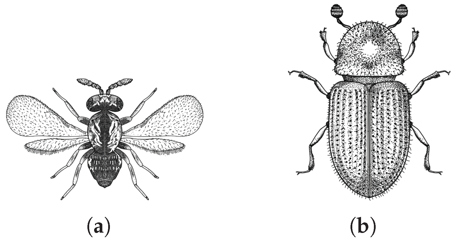
The proposed PHA-MD algorithm is inspired by the parasitic symbiotic relationship between the parasitoid wasp (Phymastichus coffea, LaSalle, Hymenoptera: Eulophidae, Figure 1a) and the coffee borer (Hypothenemus hampei, Ferrari, Coleoptera: Curculionidae: Scolytinae, Figure 1b). This symbiotic relationship is used as a biological control mechanism because the borer is considered the most harmful pest affecting the coffee crop due to its attack on the berry, producing weight loss, depreciation of the grain, and loss of quality due to the presence of impurities in the infected beans [41].

The life cycle of the wasp begins when P. coffea parasitizes H. hampei, depositing up to two eggs per host, typically one male and one female. From this point, the incubation process begins. Upon hatching, the larvae feed on the abdominal tissues of the host, the coffee borer, until they complete their metamorphosis. Once this stage is finished, the larvae emerge from the host as adult wasps [42].

The i-th symbiotic relationship ${\varphi }_i\left(t\right)$ between the i-th agents P. coffea and H. hampei at iteration t is represented as

$${\varphi }_i\left(t\right)=\{F_i\left(t\right),h_i\left(t\right),{\mathbf{p}}_i\left(t\right),{\mathbf{h}}_i\left(t\right)\},$$

(13)

where ${\mathbf{p}}_i\in {\mathbb{N}}^{j\in [1,N_n]}$ and ${\mathbf{h}}_i\in {\mathbb{R}}^{N_n}$ are the i-th agents P. coffea and H. hampei respectively, whose populations are defined as

$$\begin{array}{ccc}P\left(t\right)=\left\{\begin{array}{c}{\mathbf{p}}_1\left(t\right)\\ ⋮\\ {\mathbf{p}}_{N_a}\left(t\right)\end{array}\right\},& & H\left(t\right)=\left[\begin{array}{c}{\mathbf{h}}_1\left(t\right)\\ ⋮\\ {\mathbf{h}}_{N_a}\left(t\right)\end{array}\right]\end{array},$$

(14)

where $N_a$ is the number of agents for both populations. $F_i\left(t\right)$ is a penalty function, defined as

$$F_i\left(t\right)=E_{t_0}\left(\mathcal{U}\right)+{\alpha }_1{c}_i^{\left(1\right)}\left(t\right)+{\alpha }_2\Lambda \left({\mathbf{h}}_i\left(t\right)\right),$$

(15)

where ${\alpha }_1$ and ${\alpha }_2$ are penalty parameters, with the difference between them defining the importance between the second and third terms in (15); $c_i^{\left(1\right)}=\mathrm{card}\left({\mathbf{p}}_i\right)$ is the cardinality of the agent ${\mathbf{p}}_i\left(t\right)$; and $\Lambda \left({\mathbf{h}}_i\left(t\right)\right)$ is the maximum value between zero and the maximum real eigenvalue of matrix (11), defined as follows:

$$\Lambda \left({\mathbf{h}}_i\left(t\right)\right)={[max\left\{R_e\left\{\lambda \left\{Q(\Theta ,G,K_i)\right\}\right\}\right\}]}^{+},$$

(16)

where the elements $k_{i,j}$ of the main diagonal of the i-th control gains matrix $K_i$ are determined by the relationship of the agents ${\mathbf{p}}_i$ and ${\mathbf{h}}_i$, such that

$$k_{i,j}=\left\{\begin{array}{cc}{h}_{i,j}\hfill & j\in {\mathbf{p}}_i\hfill \\ 0\hfill & j\notin {\mathbf{p}}_i.\hfill \end{array}\right.$$

(17)

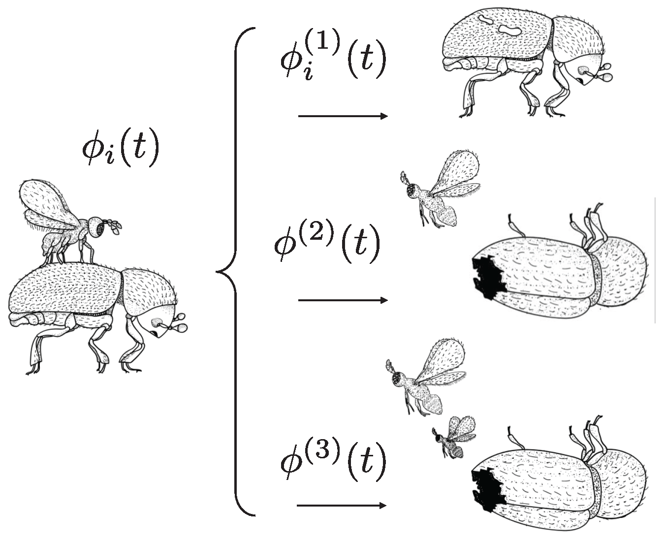
The symbiotic relationship $\varphi$ is classified in three possible favorable events for the P. coffea species (see Figure 2), which are as follows:

$${\varphi }_i^{\left(1\right)}\left(t\right)=\{F_i^{\left(1\right)}\left(t\right),{\Lambda }_i^{\left(1\right)}\left(t\right),{\mathbf{p}}_i^{\left(1\right)}\left(t\right),{\mathbf{h}}_i^{\left(1\right)}\left(t\right)\},$$

(18)

$${\varphi }^{\left(2\right)}\left(t\right)=\{F^{\left(2\right)}\left(t\right),{\Lambda }^{\left(2\right)}\left(t\right),{\mathbf{p}}^{\left(2\right)}\left(t\right),{\mathbf{h}}^{\left(2\right)}\left(t\right)\},$$

(19)

$${\varphi }^{\left(3\right)}\left(t\right)=\{F^{\left(3\right)}\left(t\right),{\Lambda }^{\left(3\right)}\left(t\right),{\mathbf{p}}^{\left(3\right)}\left(t\right),{\mathbf{h}}^{\left(3\right)}\left(t\right)\},$$

(20)

where ${\varphi }_i^{\left(1\right)}\left(t\right)$ is the favorable parasitization event, when the wasp parasites the beetle; ${\varphi }^{\left(2\right)}\left(t\right)$ implies the birth of only a female; and ${\varphi }^{\left(3\right)}\left(t\right)$ corresponds to the birth of a female and a male. Note that types 2 and 3 affect the entire population; however, type 1 is particular for each agent, and this is reflected in the subscript i for this type of symbiotic relationship. A single male fertilizes numerous females; however, it requires a female to bore the host abdomen in order to emerge, and therefore, the birth of a female and a male is the ideal scenario for the P. coffea species [42].

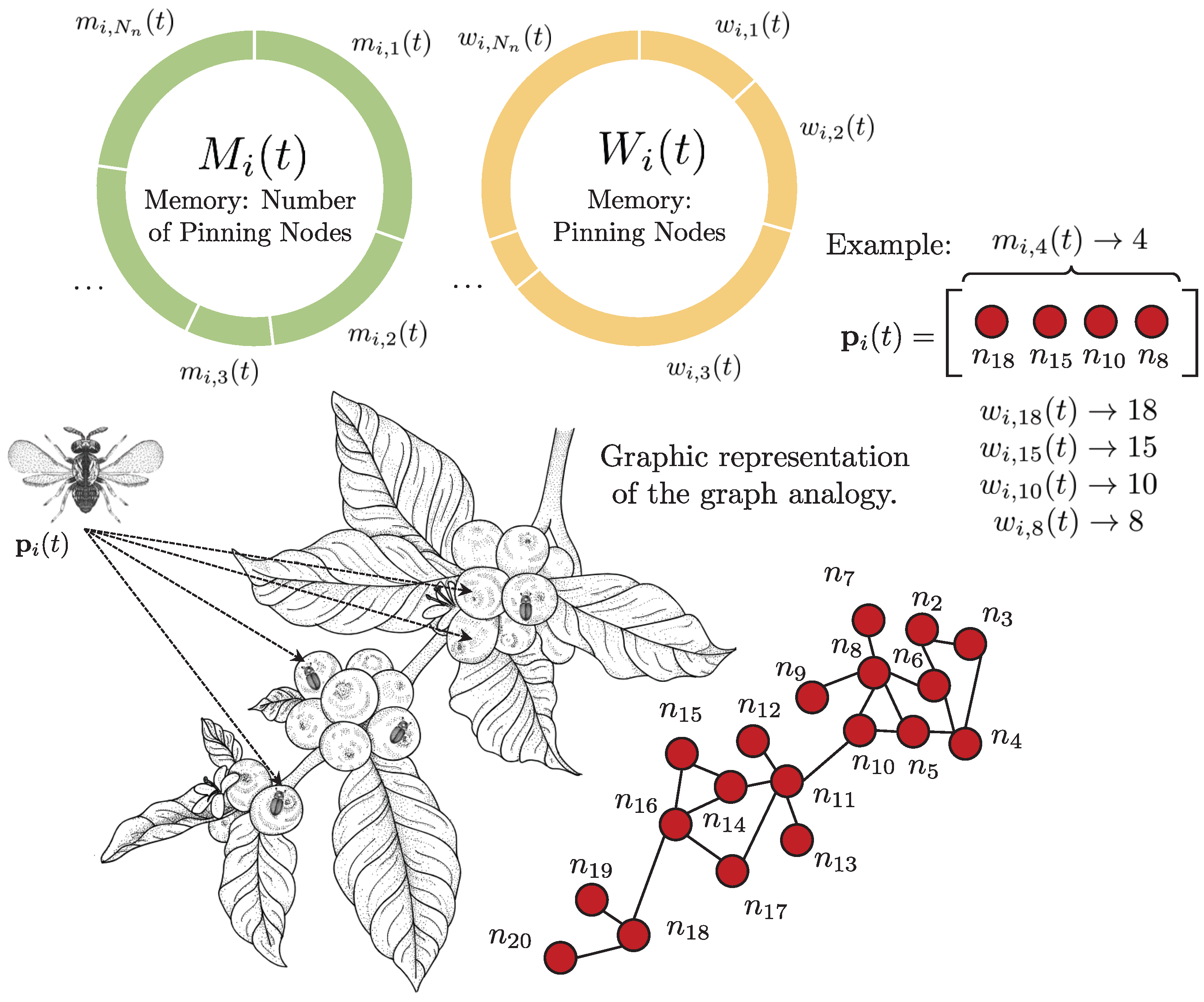
The concept of Memory Inheritance justifies the relevance of these events. This attribute implies that each i-th wasp can pass down two types of memories, ${\mathbf{m}}_i\in {\mathbb{N}}^{N_n}$ and ${\mathbf{w}}_i\in {\mathbb{R}}^{N_n}$, to its future generations. Since the coffee tree can be modeled as a graph, whose berries are equivalent to nodes, $\mathbf{m}$ and $\mathbf{w}$ are, respectively, “how many nodes to select” and “which nodes to select”.

The example in Figure 3 shows the decision of the i-th agent ${\mathbf{p}}_i\left(t\right)$ to visit four nodes, selecting $n_{18}$, $n_{15}$, $n_{10}$, and $n_8$. The elements $m_{i,j}$ and $w_{i,j}$ of each memory are selected by the roulette method. Note that in case of $m_{i,j}\left(t\right)\ne j$ or $w_{i,j}\left(t\right)\ne i$, if the element is selected, it returns the index it represents, and not its occurrence value. In the following sections, the process of modifying the frequency of occurrence is explained.

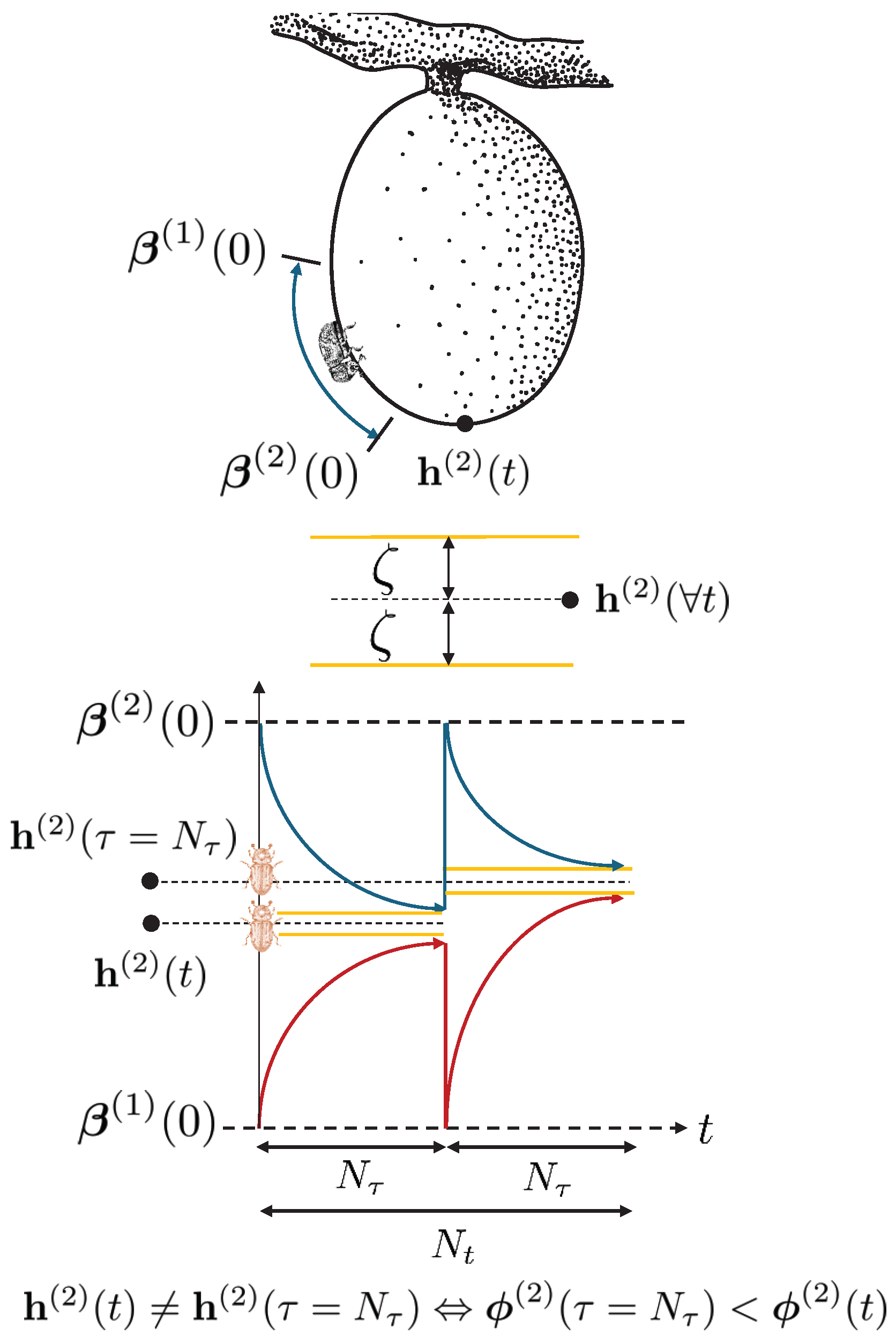
Another attribute of biological inspiration is the behavior of H. hampei. In nature, the beetle drills into coffee berries at or near the apex, which is the softest area of the coffee bean [43] (Figure 4). Similar to how the gravity, shape, relief, or orientation of the berry influence its movement, the borer functions guide H. hampei towards the optimal regions identified by the group of beetles, without direct interference. These functions reduce the search space in favor of the symbiotic relationship ${\varphi }^{\left(2\right)}$, because the beetles that manage to bore into the fruit will be able to feed, thereby increasing the probability that at least one P. coffea individual will be born. The borer functions are defined as

$$\begin{array}{cc}\hfill & {\mathit{\beta }}^{\left(1\right)}={\mathbf{h}}^{\left(2\right)}-\zeta \left|{\mathbf{h}}^{\left(2\right)}\right|+\left({\mathit{\beta }}^{\left(1\right)}\left(0\right)-{\mathbf{h}}^{\left(2\right)}+\zeta \left|{\mathbf{h}}^{\left(2\right)}\right|\right)e^{\left(\frac{-\gamma \tau }{N_{\tau }}\right)},\hfill \end{array}$$

(21)

$${\mathit{\beta }}^{\left(2\right)}={\mathbf{h}}^{\left(2\right)}+\zeta \left|{\mathbf{h}}^{\left(2\right)}\right|-\left({\mathbf{h}}^{\left(2\right)}-{\mathit{\beta }}^{\left(2\right)}\left(0\right)+\zeta \left|{\mathbf{h}}^{\left(2\right)}\right|\right)e^{\left(\frac{-\gamma \tau }{N_{\tau }}\right)},$$

(22)

where ${\mathit{\beta }}^{\left(1\right)}$ and ${\mathit{\beta }}^{\left(2\right)}$ are the lower and upper borer functions, respectively; ${\beta }_j^{\left(1\right)}\le h_{i,j}\le {\beta }_j^{\left(2\right)}\forall j\in [1,N_n]$, $\left|·\right|$ denotes the absolute value; $\zeta$ is the compression parameter, which prevents the limits ${\mathit{\beta }}^{\left(2\right)}$ and ${\mathit{\beta }}^{\left(1\right)}$ from converging to ${\mathbf{h}}^{\left(2\right)}$; $N_{\tau }$ is the maximum interaction number per epoch; $\gamma$ is an iteration coefficient; and ${\mathit{\beta }}^{\left(1\right)}\left(0\right)$ and ${\mathit{\beta }}^{\left(2\right)}\left(0\right)$ are, respectively, the initial upper and lower bounds. It is important to mention that the borer functions limit the values of each dimension j; however, they can be specific for each i-th agent H. hampei. It should be understood that with the notation of (21) and (22), the entire population H is delimited equally.

3.2. Attribute Updating

This section describes the creation of new generations for each type of agent based on updating parameters such as symbiotic relationships, updating subtypes, and optimizing inheritance memories. The subtypes of symbiotic relationships are updated as follows:

$${\varphi }_i^{\left(1\right)}\left(t\right)=\left\{\begin{array}{cc}{\varphi }_i\left(t\right)\hfill & \mathbf{if}t=1\vee \tau =1\hfill \\ {\varphi }_i\left(t\right)\hfill & \mathbf{if}t>1\wedge \tau >1\wedge F_i\left(t\right)<F_i^{\left(1\right)}(t-1)\hfill \\ {\varphi }_i^{\left(1\right)}(t-1)\hfill & \mathbf{else},\hfill \end{array}\right.$$

(23)

$${\varphi }^{\left(2\right)}\left(t\right)=\left\{\begin{array}{cc}{\varphi }_{min}^{\left(1\right)}\left(t\right)\hfill & \mathbf{if}t=1\vee \tau =1\hfill \\ {\varphi }_{min}^{\left(1\right)}\left(t\right)\hfill & \mathbf{if}t>1\wedge \tau >1\wedge F_{min}^{\left(1\right)}\left(t\right)<F^{\left(2\right)}(t-1)\hfill \\ {\varphi }^{\left(2\right)}(t-1)\hfill & \mathbf{else},\hfill \end{array}\right.$$

(24)

$${\varphi }^{\left(3\right)}\left(t\right)=\left\{\begin{array}{cc}{\varphi }^{\left(2\right)}\left(t\right)\hfill & \mathbf{if}\tau =N_{\tau }\wedge \mathcal{B}\left(t\right)=\varnothing \wedge {\mathbf{h}}^{\left(2\right)}\left(t\right)=0\hfill \\ {\varphi }^{\left(2\right)}\left(t\right)\hfill & \mathbf{if}\tau =N_{\tau }\wedge \mathcal{B}\left(t\right)\ne \varnothing \wedge {\mathbf{h}}^{\left(2\right)}\left(t\right)=0\wedge c^{\left(2\right)}\left(t\right)<c^{\left(3\right)}(t-1)\hfill \\ {\varphi }^{\left(2\right)}\left(t\right)\hfill & \mathbf{if}\tau =N_{\tau }\wedge \mathcal{B}\left(t\right)\ne \varnothing \wedge {\mathbf{h}}^{\left(2\right)}\left(t\right)=0\wedge c^2\left(t\right)=c^3(t-1)\hfill \\ \hfill & \wedge F^{\left(2\right)}\left(t\right)<F^{\left(3\right)}(t-1)\hfill \\ {\varphi }^{\left(3\right)}(t-1)\hfill & \mathbf{else},\hfill \end{array}\right.$$

(25)

where $\tau$ is the epoch trigger, which increases by one with each iteration t. When $\tau =N_{\tau }$, a new epoch starts, whose first generation has its initial conditions reset, including the epoch trigger (Figure 4), $F_{min}^{\left(1\right)}\left(t\right)={min}_{i\in \left[1,N_a\right]}\left\{F_i^{\left(1\right)}\left(t\right)\right\}$.

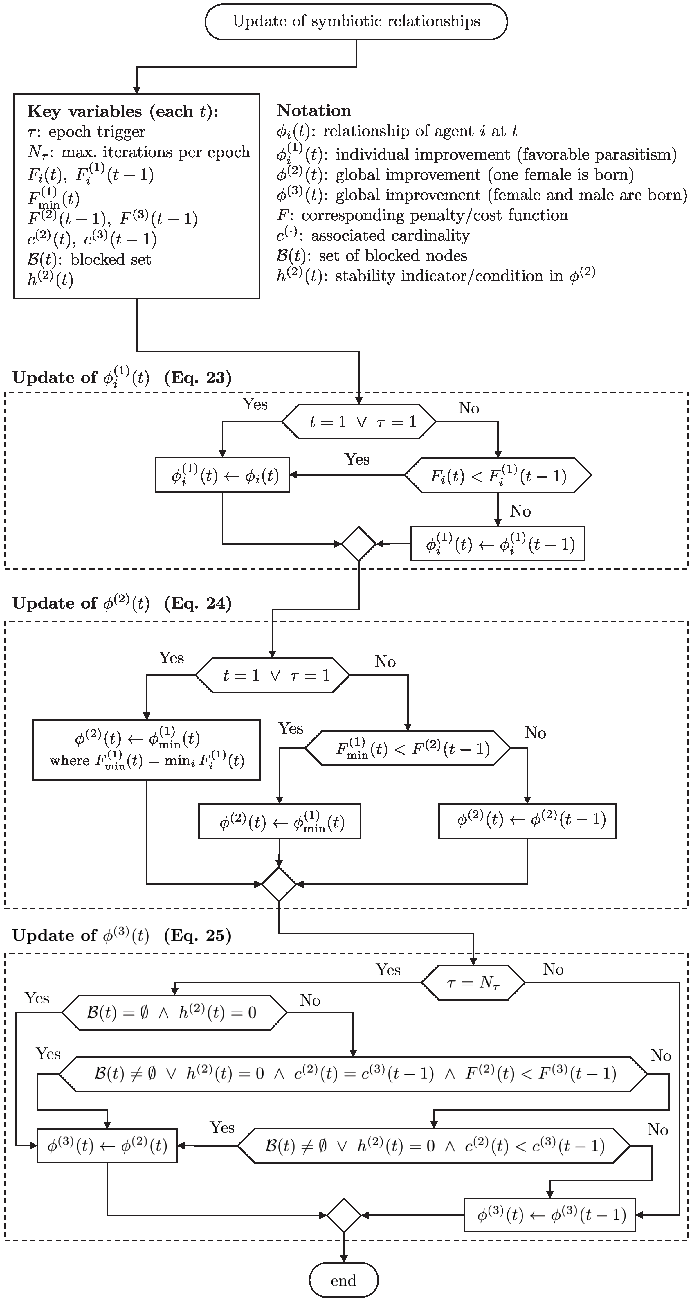
Figure 5 details how PHA-MD updates the three symbiotic subtypes at each iteration and at the end of every epoch. First, each agent evaluates its candidate and updates the per-agent best ${\varphi }_i^{\left(1\right)}\left(t\right)$ whenever its current cost $F_i\left(t\right)$ improves (Equation (23)). Next, the algorithm promotes the population-wide best ${\varphi }^{\left(2\right)}\left(t\right)$ using the minimum among $\left\{F_i^{\left(1\right)}\left(t\right)\right\}$ (Equation (24)). When the epoch boundary is reached ($\tau =N_{\tau }$), the blocking stage is invoked; based on stability ($h^{\left(2\right)}=0$), cardinality, and cost, ${\varphi }^{\left(2\right)}\left(t\right)$ may be adopted as the epoch-level best ${\varphi }^{\left(3\right)}\left(t\right)$ (Equation (25)). If the stated conditions are not met, the corresponding records are preserved (“else” branches in Equations (23)–(25)). While the flow focuses on $\varphi$-updates, it is coordinated with the blocking-set dynamics $\mathcal{B}\left(t\right)$ (Equations (26) and (27)) that are executed at epoch end.

In the PHA-MD algorithm, a new feature has been introduced compared to its previous version, a node-blocking stage. This stage involves the identification and blocking of nodes, with the set of blocked nodes denoted as $\mathcal{B}\left(t\right)$. During each epoch, if and only if $h^{\left(1\right)}\left(t\right)=0$, a node will be selected for blocking. This action increases the cardinality of the set $\mathcal{B}\left(t\right)$ by one. The set $B\left(t\right)$ captures the nodes that are currently blocked at time t, reflecting the evolving state of the algorithm as it progresses through each epoch. The set of blocked nodes is defined as

$$\mathcal{B}\left(t\right)=\left\{\begin{array}{cc}\varnothing \hfill & \mathbf{if}t<N_{\tau }\hfill \\ b\left(t\right)\hfill & \mathbf{if}\tau =N_{\tau }\wedge b\left(t\right)=\varnothing \wedge h^{\left(2\right)}\left(t\right)=0\hfill \\ \mathcal{B}(t-1)\cup b\hfill & \mathbf{if}\tau =N_{\tau }\wedge \mathcal{B}\left(t\right)\ne \varnothing \wedge h^{\left(2\right)}\left(t\right)=0\wedge N_n-c^{\left(\mathcal{B}\right)}>N_{{\lambda }^{+}}\hfill \\ {\mathcal{B}}_{max}\left(t\right)\hfill & \mathbf{if}\tau =N_{\tau }\wedge \mathcal{B}\left(t\right)\ne \varnothing \wedge h^{\left(2\right)}\left(t\right)\ne 0\hfill \\ \mathcal{B}(t-1)\hfill & \mathbf{else},\hfill \end{array}\right.$$

(26)

where $b\left(t\right)$ is a blocked node, and ${\mathcal{B}}_{max}\left(t\right)$ is the best set of blocked nodes, such that

$${\mathcal{B}}_{max}\left(t\right)=\left\{\begin{array}{cc}\varnothing \hfill & \mathbf{if}t<N_{\tau }\hfill \\ \mathcal{B}(t-1)\hfill & \mathbf{if}\tau =N_{\tau }\wedge \mathcal{B}\left(t\right)=\varnothing \wedge h^{\left(2\right)}\left(t\right)=0\hfill \\ \mathcal{B}(t-1)\hfill & \mathbf{if}\tau =N_{\tau }\wedge \mathcal{B}\left(t\right)\ne \varnothing \wedge h^{\left(2\right)}\left(t\right)=0\wedge c^{\left(\mathcal{B}\right)}\ge c^{\left({\mathcal{B}}_{max}\right)}\hfill \\ {\mathcal{B}}_{max}(t-1)\hfill & \mathbf{else},\hfill \end{array}\right.$$

(27)

with $c^{\left(\mathcal{B}\right)}=\mathrm{card}\left(\mathcal{B}\right)$ and $c^{\left({\mathcal{B}}_{max}\right)}=\mathrm{card}\left({\mathcal{B}}_{max}\right)$. The i-th node will be blocked when its number of visits implies the minimum number of successes achieved, thus

$$b\left(t\right)=\underset{i\in \left[1,N_n\right]}{max}\left\{\sum _{j=1}^{N_a}{\displaystyle \frac{v_{i,j}\left(t\right)}{w_{i,j}\left(t\right)}}\right\},$$

(28)

where $v_{i,j}\left(t\right)$ represents the number of visits made by the i-th agent of P. coffea at the j-th node. A visit by this agent is considered successful if it leads to performance improvement. The memory vector ${\mathbf{w}}_i\left(t\right)\in {\mathbb{R}}^{1\times N_n}$ increases its j-th dimension by 1 to signify successful visits.

In this context, $v_{i,j}\left(t\right)$ accounts for both successful and unsuccessful visits, while $w_{i,j}\left(t\right)$ specifically tracks successful visits by incrementing its j-th dimension when the i-th agent enhances its performance after visiting the j-th node. As shown in Figure 3, the first type of memory that P. coffea agents inherit from their offspring is $M\in {\mathbb{R}}^{N_a\times N_n}$. This memory represents “how many nodes to select”, that is, the cardinality of each agent, and its elements $m_{i,j}\left(t\right)$ are updated in the following way:

$$m_{i,j}(t+1)=\left\{\begin{array}{cc}1\forall i\hfill & \mathbf{if}t=1\wedge j>N_{{\lambda }^{+}}\hfill \\ 0\forall i\hfill & \mathbf{if}t=1\wedge j\le N_{{\lambda }^{+}}\hfill \\ m_{i,j}\left(t\right)+1\hfill & \mathbf{if}{F}_i^{\left(1\right)}\left(t\right)<F_i^{\left(1\right)}(t-1)\wedge j=c^{\left(1\right)}\left(t\right)\hfill \\ 0\forall i\hfill & \mathbf{if}{\mathbf{h}}_i^{\left(1\right)}\left(t\right)=0\wedge j>c^{\left(1\right)}\left(t\right)\hfill \\ 1\forall i\hfill & \mathbf{if}\tau =N_{\tau }\wedge j\in [N_n-c^{\left(\mathcal{B}\right)}-1,N_n-c^{\left(\mathcal{B}\right)}]\hfill \\ 0\forall i\hfill & \mathbf{if}\tau =N_{\tau }\wedge j\notin [N_n-c^{\left(\mathcal{B}\right)}-1,N_n-c^{\left(\mathcal{B}\right)}]\hfill \\ m_{i,j}\left(t\right)\hfill & \mathbf{else},\hfill \end{array}\right.$$

(29)

where $c^{\left(1\right)}\left(t\right)=\mathrm{card}\left({\mathbf{p}}_i^{\left(1\right)}\left(t\right)\right)$. The second type of memory that P. coffea agents inherit from their offspring is $W\in {\mathbb{R}}^{N_a\times N_n}$. This memory represents “which nodes to select”, and its elements $w_{i,j}\left(t\right)$ are updated in the following way:

$$w_{i,j}(t+1)=\left\{\begin{array}{cc}1\hfill & \mathbf{if}t=1\hfill \\ w_{i,j}\left(t\right)+1\hfill & \mathbf{if}{F}_i^{\left(1\right)}\left(t\right)<F_i^{\left(1\right)}(t-1)\wedge j\in {\mathbf{p}}_i^{\left(1\right)}\left(t\right)\hfill \\ w_{i,j}\left(t\right)+1\hfill & \mathbf{if}{F}^{\left(2\right)}\left(t\right)<F^{\left(2\right)}(t-1)\wedge i\in \mathcal{R}\left(t\right)\wedge j\in {\mathbf{p}}^{\left(2\right)}\left(t\right)\hfill \\ 0\forall i\hfill & \mathbf{if}\tau =N_{\tau }\wedge j\in \mathcal{B}\left(t\right)\hfill \\ 1\forall i\hfill & \mathbf{if}\tau =N_{\tau }\wedge j\notin \mathcal{B}\left(t\right)\hfill \\ w_{i,j}\left(t\right)\hfill & \mathbf{else},\hfill \end{array}\right.$$

(30)

where $\mathcal{R}\left(t\right)$ is a set of uniformly distributed random nodes (without repetition) with random cardinality.

3.3. Saturated Sigmoid Switch Functions

Saturated sigmoids are employed as compact binary comparators (switches) with explicit tie handling through a small $ϵ>0$. The parameter $ϵ$ is taken as a fixed tolerance (machine epsilon, eps) and is used to disambiguate equalities [44]. Let $x=(a-b)$ denote the comparison residual. The ideal steep-slope limit is indicated by “$·\infty$” (in code, a large gain $g\gg 1$ is used).

$$S_1\left(x\right)={\displaystyle \frac{1}{1+e^{(x+ϵ)·\infty }}}=\left\{\begin{array}{cc}1,\hfill & x<0,\hfill \\ 0,\hfill & x>0,\hfill \\ 0,\hfill & x=0,\hfill \end{array}\right.\text{“}<\text{”}\mathrm{switch}.$$

(31)

$$S_2\left(x\right)=1-{\displaystyle \frac{1}{1+e^{(x-ϵ)·\infty }}}=\left\{\begin{array}{cc}1,\hfill & x>0,\hfill \\ 0,\hfill & x<0,\hfill \\ 0,\hfill & x=0,\hfill \end{array}\right.\text{“}>\text{”}\mathrm{switch}.$$

(32)

$$S_3\left(x\right)={\displaystyle \frac{1}{1+e^{(x-ϵ)·\infty }}}=\left\{\begin{array}{cc}1,\hfill & x\le 0,\hfill \\ 0,\hfill & x>0,\hfill \end{array}\right.\text{“}\le \text{”}\mathrm{switch}.$$

(33)

$$S_4\left(x\right)=1-{\displaystyle \frac{1}{1+e^{(x+ϵ)·\infty }}}=\left\{\begin{array}{cc}1,\hfill & x\ge 0,\hfill \\ 0,\hfill & x<0,\hfill \end{array}\right.\text{“}\ge \text{”}\mathrm{switch}.$$

(34)

Non-constancy of the switches in the proposed rules. The value of x depends on random draws and evolving state/memory variables, so both activation and deactivation are produced:

• In the cardinality rule (Equation (35)), $S_3({\mu }_1-z_j)$ compares a uniform draw ${\mu }_1\in [0,1]$ with cumulative weights $z_j\in [0,1]$; across j, both cases $x<0$ and $x>0$ are obtained, so $S_3$ toggles. The quantity ${\sum }_q{S}_2\left(w_{i,q}\left(t\right)\right)$ counts strictly positive success weights $w_{i,q}\left(t\right)$, and $S_2$ is activated only when $w_{i,q}\left(t\right)>0$.
• In node selection (Equation (36)), $S_3({\mu }_2-z_j)$ operates analogously with a fresh ${\mu }_2\in [0,1]$ and cumulative weights derived from ${\mathbf{w}}_i\left(t\right)$, yielding both $x\le 0$ and $x>0$.
• In the clipping function (Equation (39)), $S_3({\beta }_j^{\left(2\right)}-x)$ and $S_4({\beta }_j^{\left(1\right)}-x)$ compare the current value x with the moving upper and lower bounds ${\beta }_j^{\left(2\right)}$ and ${\beta }_j^{\left(1\right)}$; depending on the outcome, x is passed through or snapped to the nearest bound.

The $ϵ$ offsets enforce a consistent tie policy: equality is included in $S_3$ (≤) and $S_4$ (≥) and excluded in $S_1$ and $S_2$. This policy is applied consistently in all the referenced rules.

3.4. Offspring: Phymastichus

This subsection delves into the process governing the generation of new offspring of P. coffea agents. As previously discussed, PHA–MD introduces the capability to block nodes, reducing the pool of available nodes. This attribute materially influences the decision-making of each P. coffea agent through the memory M. Situations may arise where the number of available nodes is fewer than the destinations desired by an agent. To avoid this condition, the cardinality of each agent ${\mathbf{p}}_i\left(t\right)$ is defined as

$$\begin{array}{cc}\hfill c_i\left(t\right)& =min\left\{\underset{j\in [1,N_n]}{min}{\displaystyle \frac{n_j}{S_3\left({\mu }_1-z_j\right)}},\sum S_2\left({\mathbf{w}}_i\left(t\right)\right)\right\},\hfill \\ \hfill {\mathbf{z}}^{\left(M\right)}& =\left[z_1,\dots ,z_{N_n}\right],z_k=\sum _{j=1}^k{\displaystyle \frac{m_{i,j}\left(t\right)}{\sum {\mathbf{m}}_i\left(t\right)}},\hfill \\ \hfill \mathbf{n}& =\left[1,\dots ,N_n\right].\hfill \end{array}$$

(35)

where $S_2\left(·\right)$ and $S_3\left(·\right)$ are the saturated sigmoid switch functions defined in Section 3.3, and ${\mu }_1\in [0,1]$ is a uniformly distributed random number. Once $c_i\left(t\right)$ is selected, the set of pinning nodes is defined (Figure 3) so that the j-th node visited by agent ${\mathbf{p}}_i\left(t\right)$ is

$$\begin{array}{cc}\hfill p_{i,j}\left(t\right)& =\underset{j\in [1,c_i\left(t\right)]}{min}{\displaystyle \frac{n_j}{S_3\left({\mu }_2-z_j\right)}},\hfill \\ \hfill {\mathbf{z}}^{\left(W\right)}& =\left[z_1,\dots ,z_{N_n}\right],z_k=\sum _{j=1}^k{\displaystyle \frac{{\omega }_j}{\sum \mathit{\omega }}},\hfill \\ \hfill \mathit{\omega }& ={\mathbf{w}}_i\left(t\right),\mathbf{n}=\left[1,\dots ,N_n\right].\hfill \end{array}$$

(36)

where $S_3\left(·\right)$ is defined in Section 3.3 and ${\mu }_2\in [0,1]$ is uniformly distributed. If node $n_j$ is selected, its corresponding $w_{i,j}\left(t\right)$ during iteration t is set to 0 so that $n_j$ is not re-selected by the same agent. The auxiliary vector $\mathit{\omega }$ is used for this purpose, allowing temporary modification without altering the original ${\mathbf{w}}_i$.

3.5. Offspring: Hypothenemus

In this subsection, the generation process of the offspring in the population $H\left(t\right)$ is described. The population $H\left(t\right)$ evolves under random perturbations and position increments, and is given by

$$h_{i,j}(t+1)=\left\{\begin{array}{cc}{\beta }_j^{\left(1\right)}\left(0\right)+\left({\beta }_j^{\left(2\right)}\left(0\right)-{\beta }_j^{\left(1\right)}\left(0\right)\right){\mu }_3,\hfill & \mathbf{if}t=1\vee \tau =1,\hfill \\ o\left(h_{i,j}\left(t\right)+{\rho }_3{\Delta }_{i,j}\left(t\right)\right),\hfill & \mathbf{else},\hfill \end{array}\right.$$

(37)

where ${\mu }_3\in [0,1]$ is uniformly distributed. The position increment of the i-th individual is

$${\Delta }_{i,j}(t+1)=\left\{\begin{array}{cc}0,\hfill & \mathbf{if}t=1\vee \tau =1,\hfill \\ {\Delta }_{i,j}\left(t\right)+{\rho }_1{\mu }_4\left(h_{i,j}^{\left(1\right)}\left(t\right)-h_{i,j}\left(t\right)\right)+{\rho }_2{\mu }_5\left(h_j^{\left(2\right)}\left(t\right)-h_{i,j}\left(t\right)\right),\hfill & \mathbf{else},\hfill \end{array}\right.$$

(38)

where ${\rho }_1$ is the local-influence constant (two-female births), ${\rho }_2$ is the global-influence constant (female–male births), ${\rho }_3$ is an inertial constant, and $({\mu }_4,{\mu }_5)\in {[0,1]}^2$ is uniformly distributed.

The clipping function $o\left(x\right)$ prevents H. hampei agents from exceeding the search space bounds:

$$o\left(x\right)=x{S}_3\left({\beta }_j^{\left(1\right)}-x\right)S_4\left({\beta }_j^{\left(2\right)}-x\right)+S_4\left({\beta }_j^{\left(1\right)}-x\right){\beta }_j^{\left(1\right)}+S_3\left({\beta }_j^{\left(2\right)}-x\right){\beta }_j^{\left(2\right)},$$

(39)

where $S_3\left(·\right)$ and $S_4\left(·\right)$ are the saturated sigmoid switch functions defined in Section 3.3. In this way, values inside the interval $[{\beta }_j^{\left(1\right)},{\beta }_j^{\left(2\right)}]$ are preserved, whereas values attempting to cross a bound are snapped to the closest limit. This mechanism ensures that the population remains within the feasible search space while adapting to the evolving influence cues.

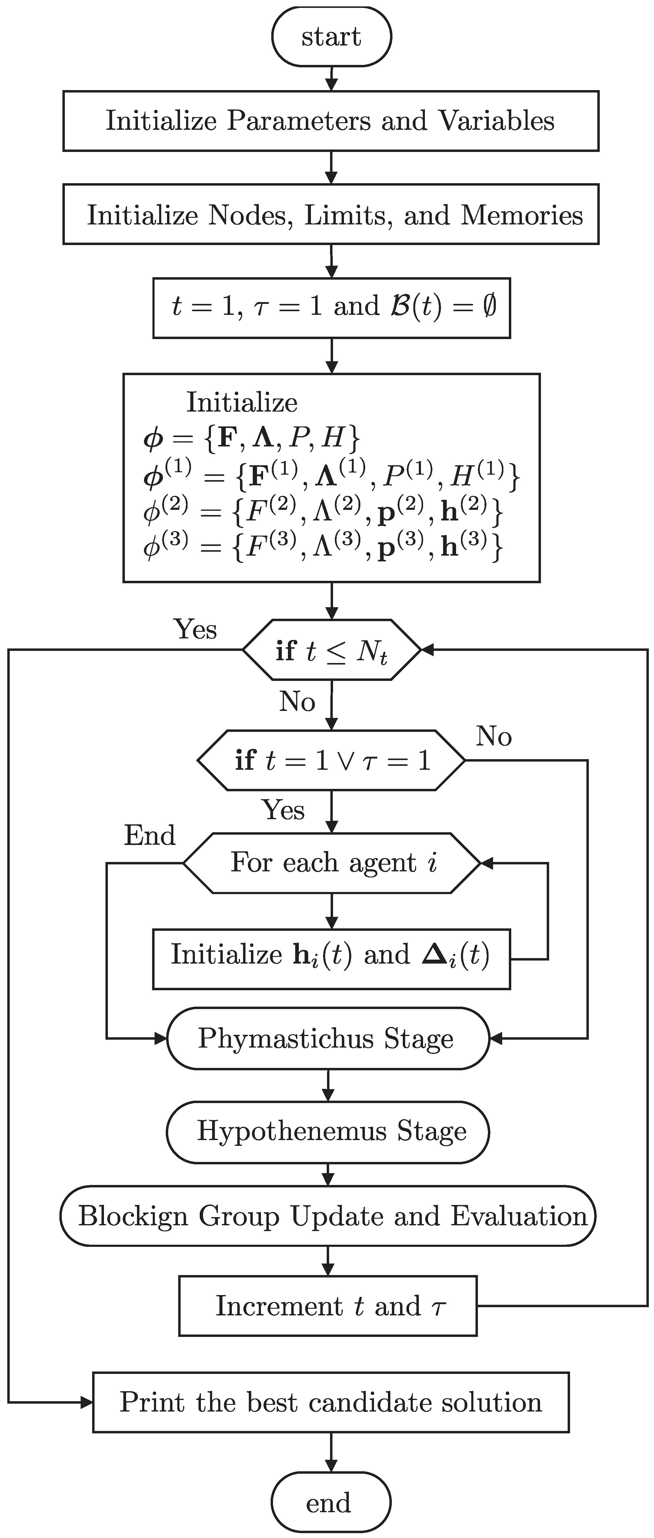
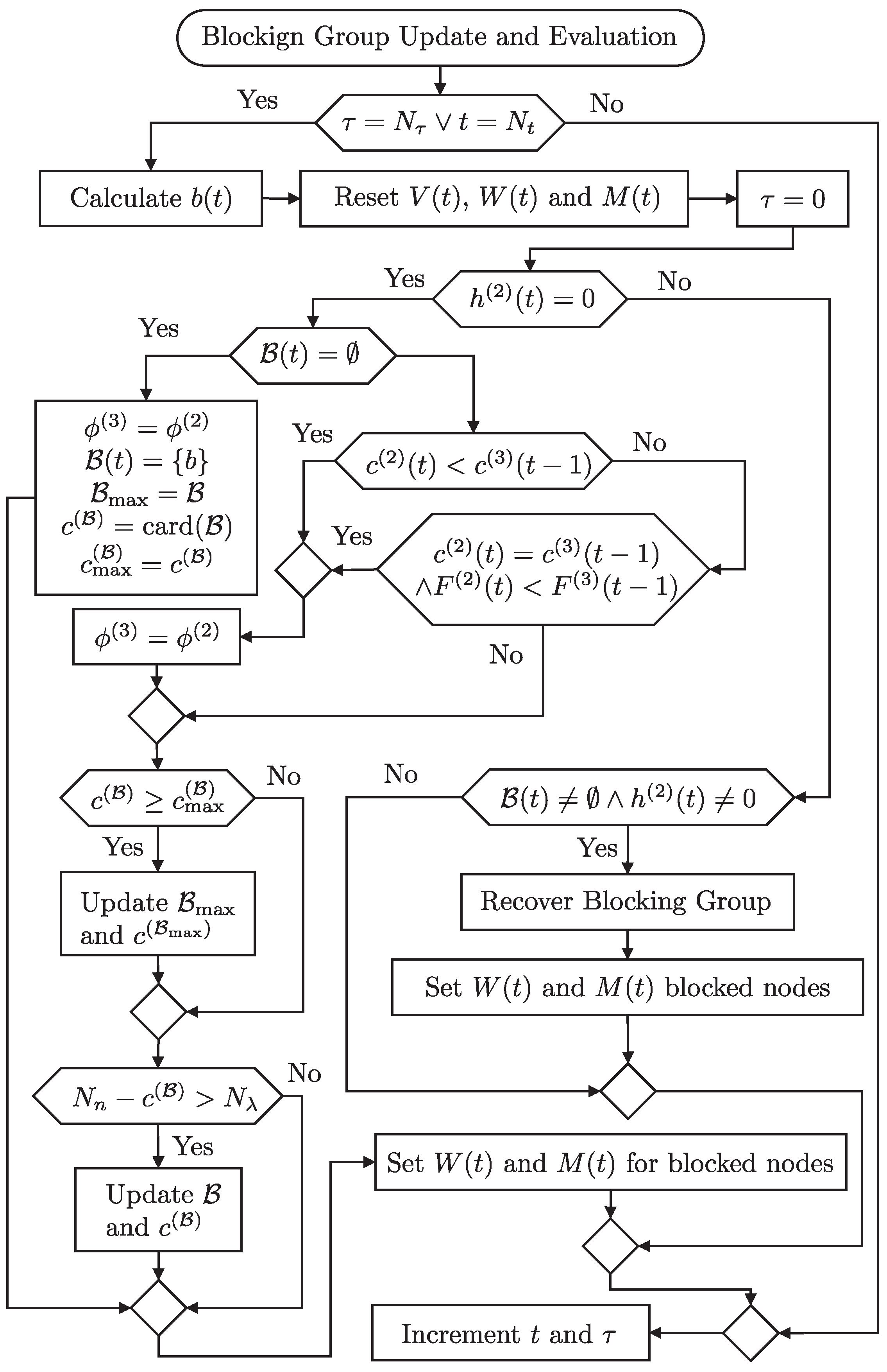
3.6. Flowchart Analysis of the PHA-MD Algorithm

Figure 6 sketches the overall control flow of PHA-MD. It highlights, at a high level, the cycle that repeats across iterations and epochs: (i) initialization at the start of each epoch; (ii) agent-driven updates—Phymastichus constructs the candidate pinning set via the inheritance memories, while Hypothenemus refines the continuous gains through the borer and clipping functions; and (iii) the epoch-end blocking step, where visits and successes are evaluated to update the blocking set. The diagram intentionally omits low-level details to emphasize data flow and stage interactions. For completeness, Algorithm 1 provides the corresponding pseudocode, aligned with Section 3, which can be read in parallel with the equations to recover the full procedural detail.

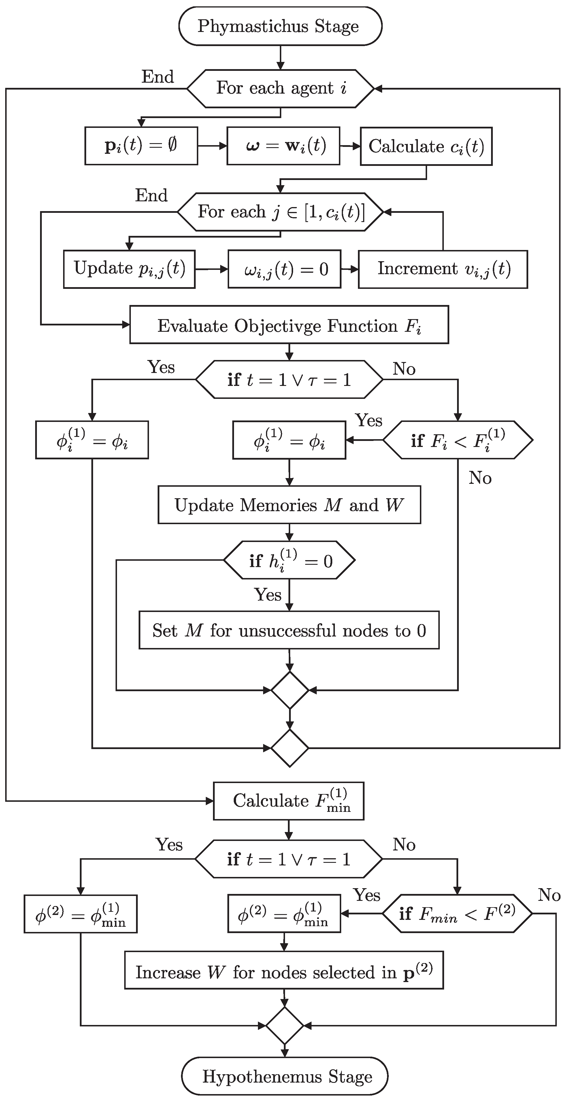
The steps that describe the Phymastichus Agent Behavior stage are as follows. “Initialization”: Each agent initializes with a random set of potential pinning. “Node Selection”: Using cumulative probabilities, the agent selects nodes to visit based on the success memories ($W\left(t\right)$) and counts ($M\left(t\right)$). “Objective Function Evaluation”: The selected nodes are evaluated using the objective function to determine their effectiveness in controlling the network. “Memory Update”: The agent updates its success memories and counts based on the evaluation results (Figure 7).

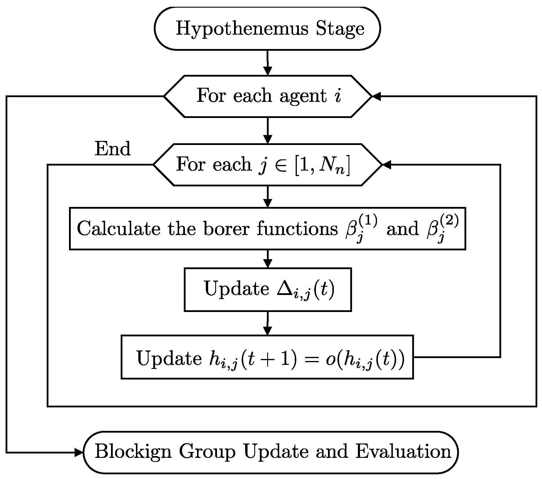
The steps that describe the Hypothenemus Agent Behavior stage are as follows. “Parameter Adjustment”: The agents adjust their parameters (${\mathit{\beta }}^{\left(2\right)}$ and ${\mathit{\beta }}^{\left(1\right)}$) using the sigmoid functions based on the iteration count. “Delta Update”: Each agent updates its delta values, incorporating local and global influences. “Node Evaluation”: Nodes are evaluated using the clipping function to ensure they remain within the bounds of ${\mathit{\beta }}^{\left(1\right)}$ and ${\mathit{\beta }}^{\left(2\right)}$. “Update Influence”: The agents update the network influence values based on their evaluations (Figure 8).

The steps that describe the Update and Evaluation of the Blocking Group stage are as follows. “Epoch Check”: The algorithm checks if the current epoch or iteration limit has been reached. “Node Blocking”: Nodes are blocked based on their visitation and success rates. “Reset Counters”: Visitation and success memories are reset for the next iteration. “Stability Check”: The algorithm checks the stability of the network and updates the best blocking group if stability is achieved. In summary, these flowcharts provide a visual representation of the PHA-MD algorithm’s structure and operations, offering insights into the systematic and iterative processes that underlie its effectiveness in optimizing pinning control for complex networks (Figure 9).

Algorithm 1 PHA-MD

Data:  $N_n,N_t,N_{\tau },N_{{\lambda }^{+}},N_a$, bounds ${\mathit{\beta }}^{\left(1\right)}\left(0\right)={\mathbf{l}}_0$, ${\mathit{\beta }}^{\left(2\right)}\left(0\right)={\mathbf{u}}_0$, $\zeta$, $({\rho }_1,{\rho }_2,{\rho }_3)$ Result:  ${\varphi }^{\left(2\right)}$ (global best), ${\varphi }^{\left(3\right)}$ (best under blocking), $\mathcal{B}$, ${\mathcal{B}}_{max}$ 1: Init:  $t\leftarrow 1,\tau \leftarrow 1,\mathcal{B}\leftarrow \varnothing ,{\mathcal{B}}_{max}\leftarrow \varnothing$ 2: $W\leftarrow {\mathbf{1}}_{N_a\times N_n}$,   $M\leftarrow {\mathbf{1}}_{N_a\times N_n}$ with $M(:,1:N_{{\lambda }^{+}})\leftarrow 0$,   $V\leftarrow \mathbf{0}$ 3: Records: $\varphi$ (current), ${\varphi }^{\left(1\right)}$ (per-agent best), ${\varphi }^{\left(2\right)}$ (global best), ${\varphi }^{\left(3\right)}$ (blocked best) 4: while  $t\le N_t$  do 5:     if $t=1$ or $\tau =1$ then                                ▹ epoch start 6:         Initialize H within $[{\mathbf{l}}_0,{\mathbf{u}}_0]$ as in Equation (37); set $\Delta \leftarrow \mathbf{0}$ 7:     end if 8:     for $i=1$ to $N_a$ do                    ▹ Phymastichus: node selection via memories 9:         Compute $Z_M=\mathrm{cumsum}\left(M(i,:)/\sum M(i,:)\right)$ 10:         $c_i\leftarrow$CardinalityBy Equation (35) using $Z_M$, $S_2$, $S_3$ 11:         $\omega \leftarrow W(i,:)$                        ▹ temporary copy to avoid reselection 12:         ${\mathbf{p}}_i\leftarrow \varnothing$ 13:         for $j=1$ to $c_i$ do 14:            $Z_W=\mathrm{cumsum}\left(\omega /\sum \omega \right)$ 15:            Select $p\leftarrow$SelectNodeBy Equation (36) using $Z_W$, $S_3$; set $\omega \left(p\right)\leftarrow 0$ ▹ no reselection 16:            ${\mathbf{p}}_i\leftarrow {\mathbf{p}}_i\cup \left\{p\right\}$;   $V(i,p)\leftarrow V(i,p)+1$ 17:         end for 18:         Evaluate $F_i,h_i$ by Equation (15); form ${\varphi }_i\left(t\right)$ (Equation (13)) 19:         Update ${\varphi }_i^{\left(1\right)}$ by Equation (23); if improved then $W(i,{\mathbf{p}}_i)+=\mathbf{1}$, $M(i,|{\mathbf{p}}_i\left|\right)+=1$ 20:         if $h_i=0$ then                              ▹ stable at current size 21:            $M(:,|{\mathbf{p}}_i|+1:N_n)\leftarrow 0$                         ▹ prune larger cardinalities 22:         end if 23:     end for 24:     Update ${\varphi }^{\left(2\right)}$ by Equation (24) using $F_{min}^{\left(1\right)}\left(t\right)$ and argmin k 25:     Broadcast ${\varphi }^{\left(2\right)}.H\leftarrow \left({\varphi }^{\left(1\right)}.H\mathrm{at}\mathrm{row}k\right)$ replicated to $N_a$ rows 26:     if ${\varphi }^{\left(2\right)}$ improved this stepthen                   ▹ as in code: only if $f_{min}$ improves 27:         Draw random subset $R\subset \{1,\dots ,N_a\}$; set $W(R,{\varphi }^{\left(2\right)}.\mathbf{p})\leftarrow W(R,{\varphi }^{\left(2\right)}.\mathbf{p})+1$ 28:     end if 29:     Hypothenemus: borer & clipping 30:     Update lower/upper bounds ${\mathit{\beta }}^{\left(1\right)},{\mathit{\beta }}^{\left(2\right)}$ by Equations (21) (lower), (22) (upper) using ${\varphi }^{\left(2\right)}.H,\zeta ,{\mathbf{l}}_0,{\mathbf{u}}_0$ 31:     $\Delta \leftarrow \Delta +{\rho }_1\mathrm{rand}\circ ({\varphi }^{\left(1\right)}.H-H)+{\rho }_2\mathrm{rand}\circ ({\varphi }^{\left(2\right)}.H-H)$                ▹ Equation (38) 32:     $H\leftarrow o\left(H+{\rho }_3\Delta ,{\mathit{\beta }}^{\left(1\right)},{\mathit{\beta }}^{\left(2\right)}\right)$                        ▹ Equation (39) with $S_3,S_4$ 33:     if $\tau =N_{\tau }$ or $t=N_t$ then                            ▹ blocking stage 34:         $b\leftarrow arg{max}_i{\sum }_j{\displaystyle \frac{V(j,i)}{W(j,i)}}$                           ▹ Equation (28) 35:         Reset epoch counters: $V\leftarrow 0,W\leftarrow \mathbf{1},M\leftarrow 0,\tau \leftarrow 0$ 36:         if ${\varphi }^{\left(2\right)}.h=0$ then                             ▹ stability at epoch end 37:            if $\mathcal{B}=\varnothing$ then 38:                ${\varphi }^{\left(3\right)}\leftarrow {\varphi }^{\left(2\right)}$;   $\mathcal{B}\leftarrow \left\{b\right\}$;   ${\mathcal{B}}_{max}\leftarrow \mathcal{B}$ 39:            else 40:                If $|{\varphi }^{\left(2\right)}.\mathbf{p}|<|{\varphi }^{\left(3\right)}.\mathbf{p}|$ or (tie & $F^{\left(2\right)}<F^{\left(3\right)}$): ${\varphi }^{\left(3\right)}\leftarrow {\varphi }^{\left(2\right)}$ 41:                If $\left|\mathcal{B}\right|\ge |{\mathcal{B}}_{max}|$: ${\mathcal{B}}_{max}\leftarrow \mathcal{B}$ 42:                if $N_n-\left|\mathcal{B}\right|>N_{{\lambda }^{+}}$ then 43:                    $\mathcal{B}\leftarrow \mathrm{unique}(\mathcal{B}\cup \{b\left\}\right)$ 44:                end if 45:            end if 46:            $W(:,\mathcal{B})\leftarrow 0$;   $M(:,N_n-|\mathcal{B}|-1:N_n-|\mathcal{B}\left|\right)\leftarrow 1$ 47:         else if $\mathcal{B}\ne \varnothing$ and ${\varphi }^{\left(2\right)}.h\ne 0$ then                  ▹ recover best blocking if no stability 48:            $\mathcal{B}\leftarrow {\mathcal{B}}_{max}$;   $W(:,\mathcal{B})\leftarrow 0$;   $M(:,N_n-|\mathcal{B}|-1:N_n-|\mathcal{B}\left|\right)\leftarrow 1$ 49:         end if 50:     end if 51:     $t\leftarrow t+1$;   $\tau \leftarrow \tau +1$ 52: end while 53: return  ${\varphi }^{\left(2\right)},{\varphi }^{\left(3\right)},\mathcal{B},{\mathcal{B}}_{max}$

3.7. Spatial Complexity Analysis

The spatial complexity of the proposed algorithm is determined by analyzing the memory usage in relation to the input parameters, specifically the number of agents $N_a$ and the number of nodes $N_n$ in the complex network. The key data structures contributing to memory consumption include matrices and cell arrays that are dynamically allocated during the algorithm’s execution.

The primary matrices W, M, V, and $\varphi$, as well as the matrices ${\mathit{\beta }}^{\left(1\right)}$ and ${\mathit{\beta }}^{\left(2\right)}$, each have a size of $N_a\times N_n$. Each of these matrices contributes $O(N_a\times N_n)$ to the spatial complexity. Since there are six such matrices, their combined complexity is $O(6\times N_a\times N_n)$.

The cell array $\mathbf{p}$, where each cell contains a vector of selected nodes, also contributes to the spatial complexity. In the worst case, the memory required is $O(N_a\times N_n)$. Additional vectors, such as F, h, and their counterparts in ${\varphi }^{\left(1\right)}$, ${\varphi }^{\left(2\right)}$, and ${\varphi }^{\left(3\right)}$, have a size of $N_a$, contributing $O(6\times N_a)$ in total. When combined, the total spatial complexity is

$$S\left(n\right)=O(6\times N_a\times N_n)+O(N_a\times N_n)+O(6\times N_a).$$

(40)

Given that the term $O(N_a\times N_n)$ dominates, the spatial complexity can be simplified to $S\left(n\right)=O(N_a\times N_n)$. This indicates that the memory usage of the algorithm increases linearly with both the number of agents and the number of nodes in the complex network, demonstrating the algorithm’s spatial efficiency.

4. Simulation Study

It is important to note that the proposed PHA-MD algorithm features variable dimensions across its agents, with each agent having a different number of dimensions. This characteristic initially precluded a direct comparison with other algorithms, such as ALO [21], TLBO [22], GWO [23], AMO [24], PSO [25], ABC [26], GSK [27], BBO [28], WOA [29], ACO [30], OOA [31], MA [32], AOA [33], CHIO [34], and DTBO [35]. These algorithms assume a fixed number of dimensions throughout the optimization process, which is not compatible with the dynamic dimensionality of PHA-MD.

The optimization problem addressed by PHA-MD involves both combinatorial and continuous elements, further complicating the use of traditional algorithms. PHA-MD was specifically designed to handle the dynamic dimensionality needed to identify the minimum number of pinning nodes, a task that requires agents to propose different sets of nodes. This flexibility in dimension handling is not supported by the aforementioned algorithms, which rely on a fixed dimension setup. For instance, initializing agents with a predefined number of dimensions for both gain constants and potential pinning nodes imposes assumptions that may not be accurate.

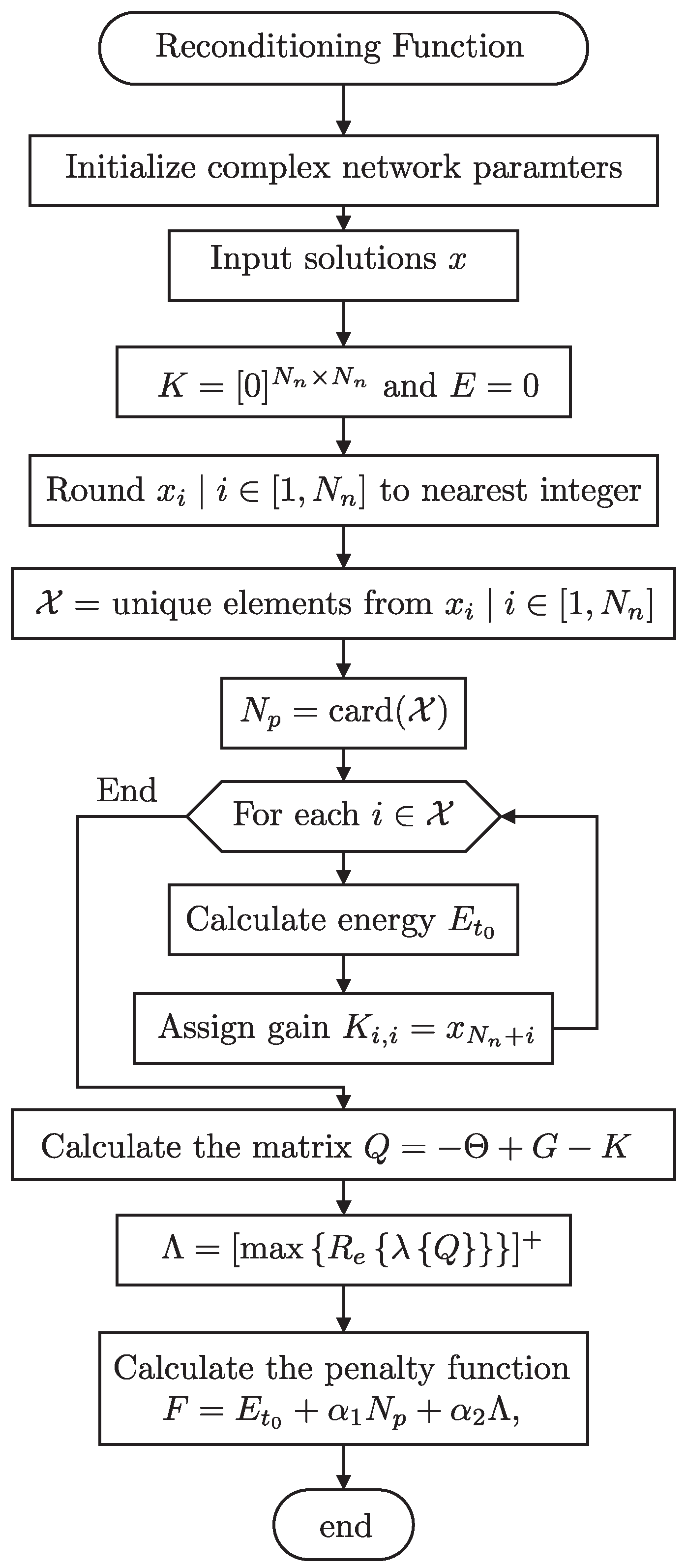
To allow a fair comparison, a reconditioning function was introduced. This function adjusts the dimensions by rounding them to the nearest integer corresponding to node indices in the matrix K and selecting unique elements. This approach standardizes the input, enabling fixed-dimension algorithms to adapt to the variable dimensionality required by PHA-MD.

All runs were performed on a single workstation under Ubuntu 22.04.3 LTS (64-bit) using MATLAB R2023b in double precision. Default multithreaded BLAS (Intel oneMKL) was enabled; GPU acceleration was not used. Randomness was controlled with MATLAB’s rng(’twister’,2024). The population size, iteration budget, and epoch length followed the values stated in Section 3, PHA-MD Algorithm, and the figure set Convergence curves for the Networks. The hardware and software stack is summarized in

Table 1. Hardware and software used for all computations.

Component	Specification
CPU	Intel Core i7-12700K (12 cores: 8P+4E, 20 threads, 3.6–5.0 GHz)
Memory	32 GB DDR4-3200
GPU	NVIDIA GeForce RTX 3060, 12 GB VRAM (not used)
Storage	1 TB NVMe SSD
Operating system	Ubuntu 22.04.3 LTS (64-bit), Linux kernel 5.15
MATLAB	R2023b (double precision)
Toolboxes	Optimization, Global Optimization; Parallel Computing (installed, disabled)
Math kernel	Intel oneMKL (default in MATLAB R2023b)
Threading	Default multithreaded linear algebra; no GPU acceleration
Random seed	rng(’twister’,2024)
Measurement	MATLAB tic/toc; single-process execution

.

Remark 2.

The number of runs required to obtain a representative solution cannot be specified a priori in a universal manner, since the selection of pinning nodes constitutes a combinatorial NP–hard problem. Consequently, the evaluation protocol is grounded in a theoretical feasibility criterion: under the V-stability of Xiang and Chen, the number of pinned nodes cannot be less than the number of non–negative eigenvalues of the characteristic matrix; thus, $N_{{\lambda }^{+}}$ is a natural lower bound. Operationally, each method was executed up to the point at which the baseline algorithms exhibited instability, whereas PHA–MD preserved feasible solutions. Accordingly, a finite iteration budget was adopted as the stopping criterion; its value was selected experimentally to reach a regime in which baseline methods typically displayed instability in their solutions, while PHA–MD continued to yield feasible trajectories. Stability therefore informs the choice of iteration budget, although simulations are not terminated upon the detection of instability itself.

Figure 10 illustrates the reconditioning function used in the simulation study. This function is essential for aligning fixed-dimension algorithms with the variable dimensionality necessary for pinning node selection in complex networks. The properties of the six complex networks analyzed are presented in

Table 2. Complex network data analyzed.

	Network 1	Network 2	Network 3	Network 4	Network 5	Network 6
$N_n$	10	20	30	40	50	60
$N_e$	18	93	224	383	653	876
$N_{{\lambda }^{+}}$	3	7	5	21	25	33
$\overline{cd}$	3.6	9.3	14.93	19.15	26.12	29.2
$min\left\{cd\right\}$	2	5	10	12	19	19
$max\left\{cd\right\}$	7	13	20	24	34	38
$\overline{c}$	10.92	5.78	9.53	−11.35	−6.90	−4.64
$I_c$	$[-4,30]$	$[-2,15]$	$[-2,20]$	$[-40,20]$	$[-24,10]$	$[-24,16]$
$\overline{\theta }$	6.69	6.31	45.93	−6.31	0.46	−7.69
$I_{\theta }$	$[-1,13]$	$[-10,15]$	$[-4,80]$	$[-23,8]$	$[-16,12]$	$[-56,35]$
${\overline{x}}_0$	$\left[\begin{array}{c}16.85\\ -10.73\\ -10.2\end{array}\right]$	$\left[\begin{array}{c}-22.13\\ 1.03\\ -12.59\end{array}\right]$	$\left[\begin{array}{c}-0.01\\ 2.02\end{array}\right]$	$\left[\begin{array}{c}2.02\\ 2.21\end{array}\right]$	$\left[\begin{array}{c}-2.33\\ -2.83\end{array}\right]$	$\left[\begin{array}{c}23.83\\ 26\\ 31.85\end{array}\right]$
$I_{x_0}$	$[-80,70]$	$[-90,55]$	$[-8,9]$	$[-2,7]$	$[-14,8]$	$[-23,80]$
$SS$	$\left[\begin{array}{c}10\\ 1\times {10}^{10}\end{array}\right]$	$\left[\begin{array}{c}1\times {10}^4\\ 2\times {10}^5\end{array}\right]$	$\left[\begin{array}{c}1\times {10}^2\\ 1\times {10}^7\end{array}\right]$	$\left[\begin{array}{c}1\times {10}^4\\ 1\times {10}^6\end{array}\right]$	$\left[\begin{array}{c}1\times {10}^5\\ 1\times {10}^7\end{array}\right]$	$\left[\begin{array}{c}1\times {10}^7\\ 1\times {10}^9\end{array}\right]$

. These properties include the number of edges ($N_e$), positive eigenvalues ($N_{{\lambda }^{+}}$), average connection degree ($\overline{cd}$), average coupling strength ($\overline{c}$), average passivity degree ($\overline{\theta }$), average initial conditions (${\overline{x}}_0$), and their respective distribution intervals ($I_{c,\theta ,x_0}$). Additionally, the search space ($SS$) defines the feasible region for selecting control gains during the optimization process.

The six synthetic networks were sampled uniformly within the intervals reported in Table 2 under two design criteria: (i) passivity degrees $\theta$ and coupling strengths $c_{ij}$ chosen to yield a nonzero count of positive eigenvalues $N_{{\lambda }^{+}}$ in the V-stability analysis, and (ii) a relatively large $N_{{\lambda }^{+}}$ compared to $N_n$, which increases the theoretical lower bound on the number of required pinning nodes. This produces challenging instances where stability is nontrivial and energy–cardinality trade-offs are visible. Although synthetic, these topologies are representative of interaction patterns commonly found in signed social influence graphs (trust/distrust) [45], neuronal microcircuits with mixed excitatory/inhibitory synapses [46], gene-regulatory subnetworks with activation/repression [47], distribution grids with grid-connected power-electronic converters exhibiting impedance interactions [48,49], and antagonistic ecological webs (predator–prey) [50]. Thus, “Network 1–6” should be read as topology classes that capture these motifs, rather than as single specific datasets.

The parameter settings used in the simulations for the various algorithms are summarized in

Table 3. The parameter settings for the algorithms used in the simulations.

Algorithm	Parameter	Value
ALO	Elite rate	0.1
	Ant rate	0.9
WOA	Convergence parameter (a)	[2, 0]
	r (random vector)	[0, 1]
	l (random number)	[−1, 1]
TLBO	$T_F$ (teaching factor)	$\left[\right(1+\mathrm{rand}\left)\right]$
	rand (random number)	[0, 1]
GWO	a (convergence parameter)	[2, 0]
	$\alpha$ (alternative parameter)	$2-2(g/{\max }_g)$
AMO	Animals in each group	5
PSO	$\mathit{\omega }$ (inertia weight)	0.6
	$c_1$, $c_2$ (cognitive and social constants)	2
ABC	Abandonment criteria	25
GSK	P (probability)	0.1
	$k_f$ (forward coeff)	0.5
	$k_r$ (return coeff)	0.9
	K (number of iters)	10
BBO	Habitat modification probability	1
	Immigration probability bounds per gene	[0, 1]
	Step size for numerical integration	1
	Max. immigration and migration rates	1
	Mutation probability	0.1
ACO	Initial pheromone value	1 × 10−6
	Pheromone update constant	20
	Exploration constant	1
	Global pheromone decay rate	0.9
	Local pheromone decay rate	0.5
	Pheromone sensitivity	1
	Visibility sensitivity	5
PHA	${\rho }_1$ (local influence coeff)	0.5
	${\rho }_2$ (global influence coeff)	0.6
	${\rho }_3$ (increment coeff)	0.7
	$\zeta$ (clustering tolerance)	0.02
	$\gamma$ (control gain)	10
OOA	Elite rate	0.2
	Infection rate	0.1
MA	Attraction rate	0.5
	Repulsion rate	0.3
AOA	Exploration rate	0.4
	Exploitation rate	0.6
CHIO	Infection probability	0.3
	Recovery probability	0.1
DTBO	Learning rate	0.1
	Feedback rate	0.2
All algorithms	Population size	50
	Number of iters	500

. For each baseline, hyperparameters were taken from the authors’ recommended operating conditions in their original sources; no per-benchmark retuning was performed to avoid overfitting to the synthetic networks. The population size and number of iterations were kept constant across all methods to enforce a common computational budget. A reconditioning wrapper was employed to standardize candidate representations so fixed-dimension heuristics could accept the variable-cardinality solutions produced by PHA–MD. Because the control objective was stability-first, candidates that failed the stability test are reported as unstable and are not considered acceptable low-energy optima. This protocol separates algorithmic design differences (fixed versus variable dimensionality with stability feedback) from hyperparameter tweaks and supports a fair comparison.

As mentioned, the performance of the proposed PHA-MD algorithm is compared with several other heuristic optimization algorithms across six different complex network topologies. These topologies were generated uniformly at random within the intervals specified in Table 2. The networks were designed to challenge current optimization algorithms and reveal scenarios where stability is difficult to achieve. The aim was to create increasingly complex networks to showcase the superior capability of the PHA-MD algorithm. If a network were encountered where even PHA-MD could not find stable solutions, the algorithm would need to be reconfigured to address these new challenges.

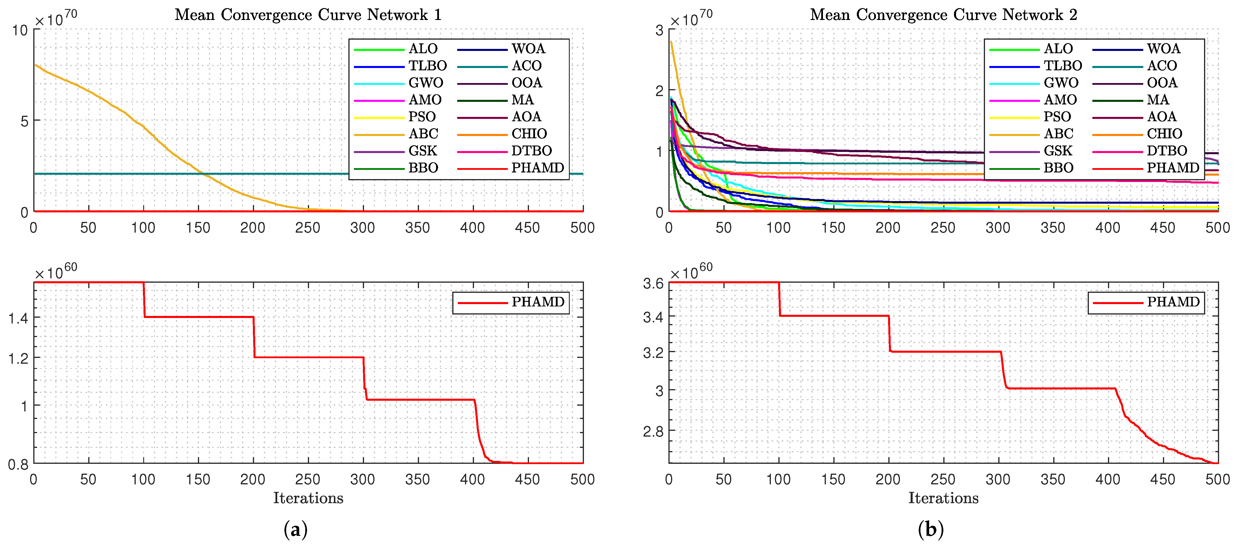
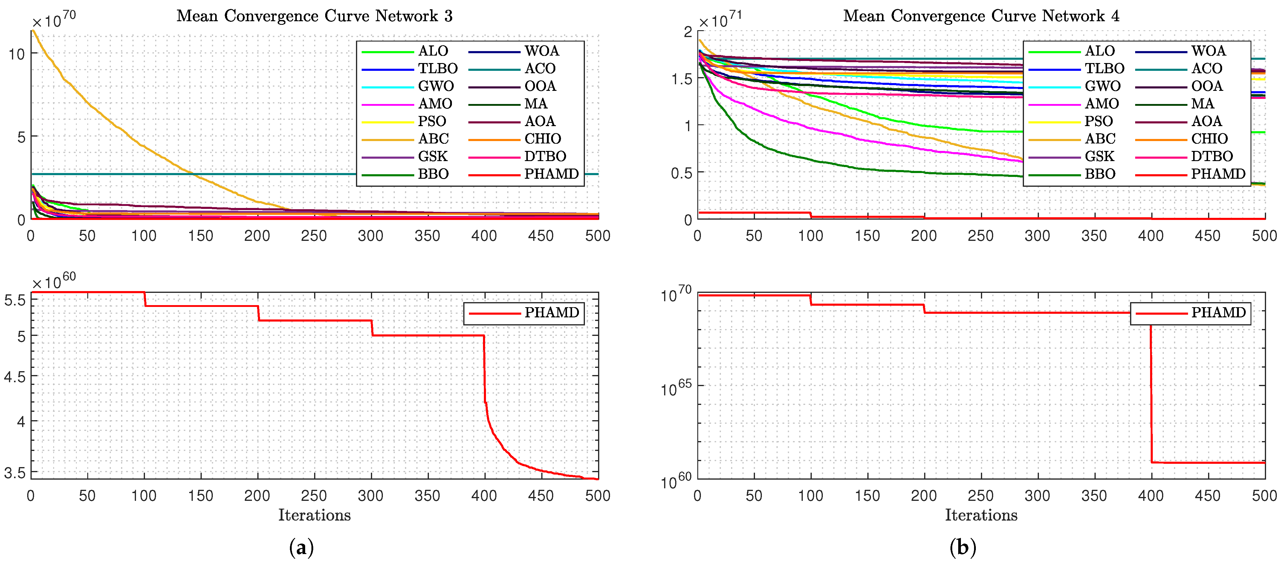
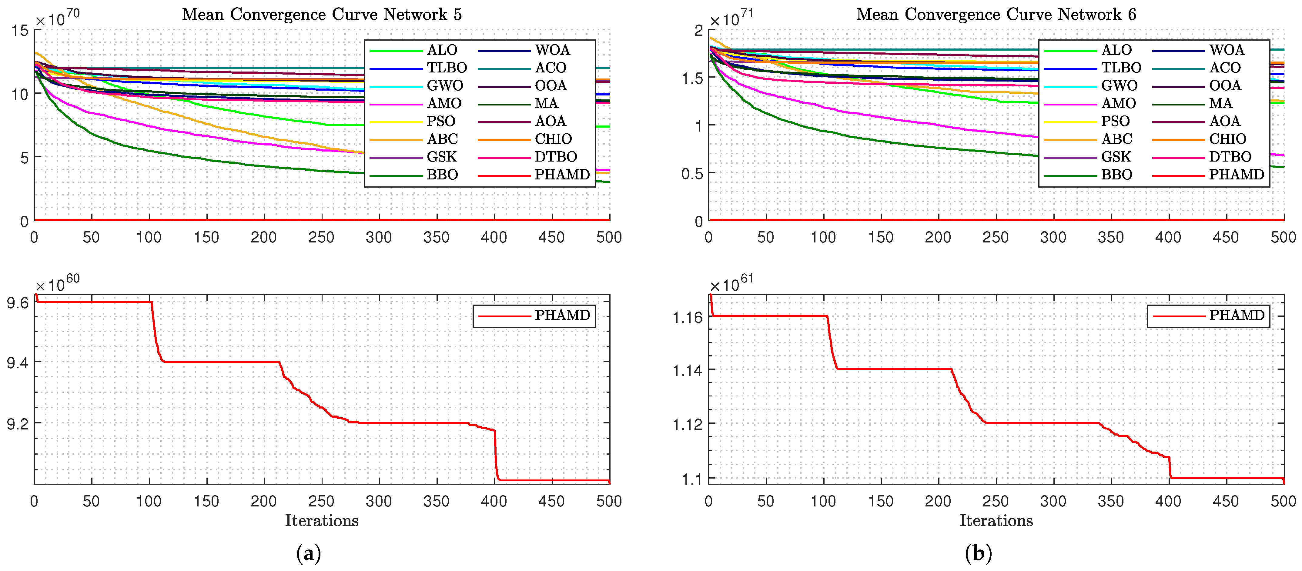
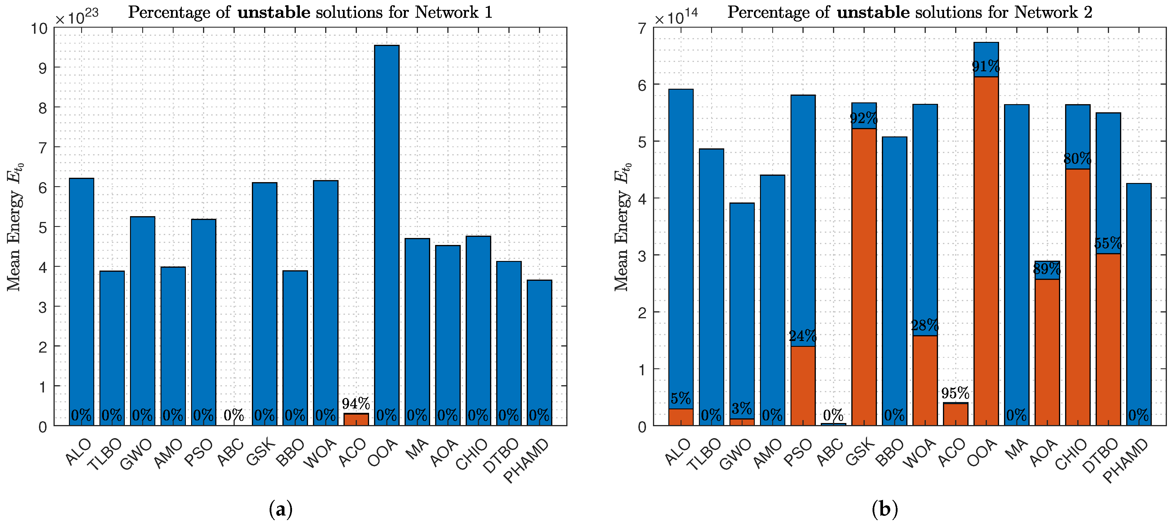
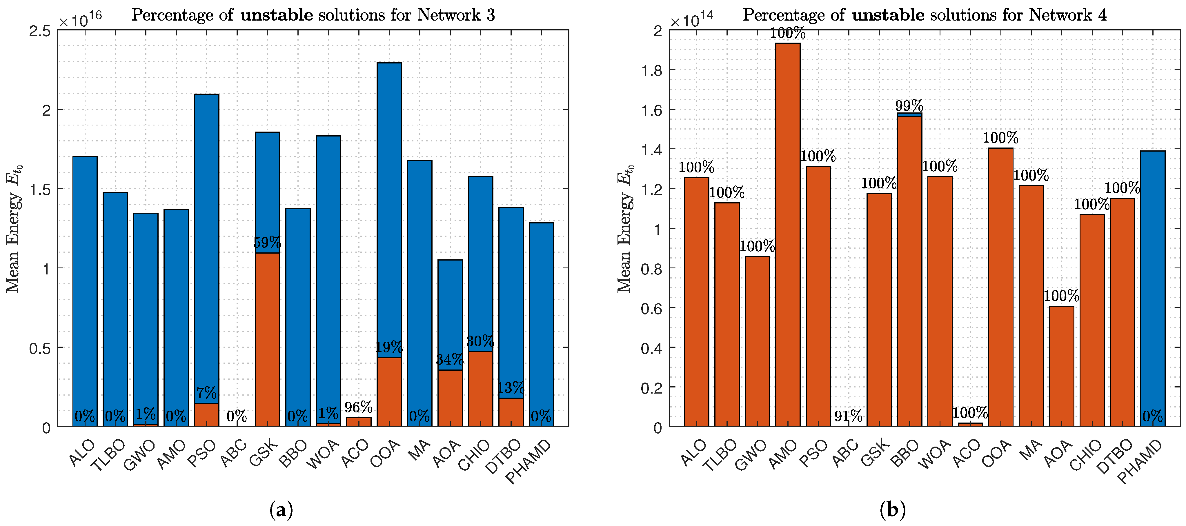
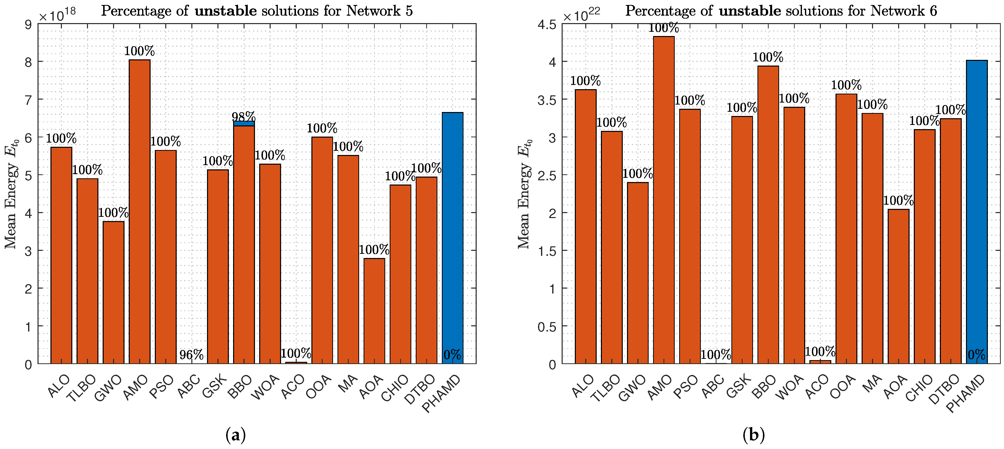
The simulation results include two sets of graphs. The first set (Figure 11, Figure 12 and Figure 13) presents the convergence curves for each network’s optimization, comparing the performance of the PHA-MD algorithm with that of other algorithms. The second set (Figure 14, Figure 15 and Figure 16) of graphs shows the optimization of energy $E_{t_0}$ against the percentage of unstable solutions, emphasizing solution stability.

In Figure 11a, the convergence behavior for Network 1 is depicted. Due to the scale, only the ABC algorithm is prominently visible, with others appearing unchanged. Figure 11b allows for a comparison across all algorithms, showing similar convergence except for in the case of GSK and ACO.

The PHA-MD algorithm reaches its minimum value earlier than others, demonstrating its efficiency. Figure 12a complicates comparisons due to the ABC algorithm’s scale, yet most algorithms show early convergence, with PHA-MD continuing to converge rapidly.

As shown in Figure 12b, the optimization process becomes more challenging due to Network 4’s size, with a clear gap between PHA-MD and the others, and only four out of five epochs observed due to unchanged candidate solutions. Figure 13a displays similar behavior, with drilling functions proving effective, and BBO and AMO following PHA-MD in performance. Finally, Figure 13b shows an even greater gap between PHA-MD and the other algorithms, highlighting PHA-MD’s superior performance in minimizing the cost function F.

In addition to the convergence curves, Figure 14, Figure 15 and Figure 16 present the optimization of energy $E_{t_0}$ against the percentage of unstable solutions. Blue bars represent the average energy consumption of each algorithm’s solutions, with percentages indicating the proportion of unstable solutions. Figure 14a shows that the ABC algorithm achieves the lowest energy consumption with 0% unstable solutions, while ACO, despite being energy-efficient, has 94% unstable solutions, highlighting the trade-off between energy efficiency and stability.

In Figure 14b, the ABC algorithm remains the most energy-efficient, but several algorithms, including ALO, GWO, PSO, WOA, GSK, and ACO, present unstable solutions, with ACO having the highest instability rate at 95%. Figure 15a shows a reduction in unstable solutions due to Network 3 having fewer states. By Figure 15b, nearly all algorithms exhibit 100% unstable solutions, despite Network 4 having the same number of states, indicating that complexity depends on more than just the number of states. Figure 16a shows some algorithms achieving stable solutions, while Figure 16b highlights that only PHA-MD provides stable solutions, underscoring its prioritization of stability over energy efficiency.

These results demonstrate the PHA-MD algorithm’s effectiveness in achieving rapid convergence and superior optimization compared to other algorithms. Its ability to handle variable dimensionality and combinatorial optimization makes it particularly suitable for pinning control in complex networks. The simulation results are summarized in

Table 4. Simulation results for different algorithms across six networks.

Algorithm	Measure	Network 1	Network 2	Network 3	Network 4	Network 5	Network 6
ALO	Avg. CF	5.1 $\times {10}^{60}$	6.8602 $\times {10}^{68}$	1.912 $\times {10}^{61}$	4.6041 $\times {10}^{71}$	3.6848 $\times {10}^{71}$	6.132 $\times {10}^{71}$
	Best CF	4 $\times {10}^{60}$	1.3 $\times {10}^{61}$	1.7 $\times {10}^{61}$	1.7079 $\times {10}^{71}$	1.6174 $\times {10}^{71}$	3.2368 $\times {10}^{71}$
	Avg. NP	5	15	19	33	40	46
	Best NP	4	13	17	30	35	40
	Avg. EC	6.2082 $\times {10}^{23}$	5.9117 $\times {10}^{14}$	1.7025 $\times {10}^{16}$	1.2553 $\times {10}^{14}$	5.7283 $\times {10}^{18}$	3.6252 $\times {10}^{22}$
	Best EC	1.1201 $\times {10}^{23}$	2.404 $\times {10}^{14}$	7.8747 $\times {10}^{15}$	3.7911 $\times {10}^{13}$	2.5242 $\times {10}^{18}$	2.3748 $\times {10}^{22}$
TLBO	Avg. CF	4 $\times {10}^{60}$	1.498 $\times {10}^{61}$	1.962 $\times {10}^{61}$	6.7339 $\times {10}^{71}$	4.942 $\times {10}^{71}$	7.6473 $\times {10}^{71}$
	Best CF	4 $\times {10}^{60}$	1.4 $\times {10}^{61}$	1.7 $\times {10}^{61}$	5.7775 $\times {10}^{71}$	3.6628 $\times {10}^{71}$	5.9984 $\times {10}^{71}$
	Avg. NP	4	15	20	31	37	43
	Best NP	4	14	17	27	33	37
	Avg. E	3.8762 $\times {10}^{23}$	4.8607 $\times {10}^{14}$	1.4766 $\times {10}^{16}$	1.1278 $\times {10}^{14}$	4.8949 $\times {10}^{18}$	3.0739 $\times {10}^{22}$
	Best E	4.5673 $\times {10}^{22}$	1.9126 $\times {10}^{14}$	8.0718 $\times {10}^{15}$	5.7146 $\times {10}^{13}$	2.0877 $\times {10}^{18}$	1.382 $\times {10}^{22}$
GWO	Avg. CF	4.75 $\times {10}^{60}$	2.4728 $\times {10}^{68}$	1.6844 $\times {10}^{67}$	6.434 $\times {10}^{71}$	4.6174 $\times {10}^{71}$	7.2403 $\times {10}^{71}$
	Best CF	4 $\times {10}^{60}$	1.2 $\times {10}^{61}$	1.8 $\times {10}^{61}$	3.745 $\times {10}^{71}$	2.6409 $\times {10}^{71}$	3.9817 $\times {10}^{71}$
	Avg. NP	5	15	20	30	37	43
	Best NP	4	12	18	26	33	37
	Avg. E	5.2435 $\times {10}^{23}$	3.9094 $\times {10}^{14}$	1.3449 $\times {10}^{16}$	8.5704 $\times {10}^{13}$	3.7608 $\times {10}^{18}$	2.3976 $\times {10}^{22}$
	Best E	8.0848 $\times {10}^{22}$	1.1117 $\times {10}^{14}$	2.5247 $\times {10}^{15}$	1.9739 $\times {10}^{13}$	1.0436 $\times {10}^{18}$	1.268 $\times {10}^{22}$
AMO	Avg. CF	4 $\times {10}^{60}$	1.282 $\times {10}^{61}$	1.653 $\times {10}^{61}$	1.8614 $\times {10}^{71}$	1.9714 $\times {10}^{71}$	3.3892 $\times {10}^{71}$
	Best CF	4 $\times {10}^{60}$	1.2 $\times {10}^{61}$	1.5 $\times {10}^{61}$	2.5401 $\times {10}^{70}$	1.624 $\times {10}^{70}$	2.0201 $\times {10}^{71}$
	Avg. NP	4	13	17	36	44	51
	Best NP	4	12	15	34	41	46
	Avg. E	3.979 $\times {10}^{23}$	4.4029 $\times {10}^{14}$	1.3695 $\times {10}^{16}$	1.9327 $\times {10}^{14}$	8.0387 $\times {10}^{18}$	4.3284 $\times {10}^{22}$
	Best E	5.5216 $\times {10}^{22}$	1.9064 $\times {10}^{14}$	7.1131 $\times {10}^{15}$	1.0368 $\times {10}^{14}$	5.0968 $\times {10}^{18}$	2.4297 $\times {10}^{22}$
PSO	Avg. CF	4.79 $\times {10}^{60}$	3.4255 $\times {10}^{69}$	1.4353 $\times {10}^{69}$	7.4066 $\times {10}^{71}$	5.4168 $\times {10}^{71}$	8.231 $\times {10}^{71}$
	Best CF	4 $\times {10}^{60}$	1.3 $\times {10}^{61}$	2 $\times {10}^{61}$	6.2805 $\times {10}^{71}$	4.7809 $\times {10}^{71}$	6.5008 $\times {10}^{71}$
	Avg. NP	5	15	22	29	35	41
	Best NP	4	13	20	24	31	35
	Avg. E	5.1762 $\times {10}^{23}$	5.8063 $\times {10}^{14}$	2.0949 $\times {10}^{16}$	1.3113 $\times {10}^{14}$	5.6448 $\times {10}^{18}$	3.3657 $\times {10}^{22}$
	Best E	4.7222 $\times {10}^{22}$	2.3678 $\times {10}^{14}$	8.6401 $\times {10}^{15}$	5.8626 $\times {10}^{13}$	3.1002 $\times {10}^{18}$	1.9188 $\times {10}^{22}$
ABC	Avg. CF	7.84 $\times {10}^{60}$	1.496 $\times {10}^{61}$	2.659 $\times {10}^{61}$	1.7899 $\times {10}^{71}$	1.8478 $\times {10}^{71}$	6.2455 $\times {10}^{71}$
	Best CF	6 $\times {10}^{60}$	1.3 $\times {10}^{61}$	2.4 $\times {10}^{61}$	3.7 $\times {10}^{61}$	4.7 $\times {10}^{61}$	3.7078 $\times {10}^{71}$
	Avg. NP	8	15	27	37	45	48
	Best NP	6	13	24	32	39	41
	Avg. E	6.0857 $\times {10}^{13}$	3.8347 $\times {10}^{12}$	2.0035 $\times {10}^7$	4.4134 $\times {10}^{10}$	1.9193 $\times {10}^{13}$	1.0839 $\times {10}^{19}$
	Best E	6.3576 $\times {10}^7$	3.3042 $\times {10}^{12}$	1.0895 $\times {10}^7$	3.7038 $\times {10}^{10}$	1.4898 $\times {10}^{13}$	8.7471 $\times {10}^{18}$
GSK	Avg. CF	5.7 $\times {10}^{60}$	4.7397 $\times {10}^{70}$	2.0125 $\times {10}^{70}$	7.9435 $\times {10}^{71}$	5.601 $\times {10}^{71}$	8.3242 $\times {10}^{71}$
	Best CF	4 $\times {10}^{60}$	1.6 $\times {10}^{61}$	1.9 $\times {10}^{61}$	6.2524 $\times {10}^{71}$	4.7282 $\times {10}^{71}$	7.0532 $\times {10}^{71}$
	Avg. NP	6	15	22	29	36	42
	Best NP	4	13	19	25	32	36
	Avg. E	6.0977 $\times {10}^{23}$	5.672 $\times {10}^{14}$	1.8551 $\times {10}^{16}$	1.1749 $\times {10}^{14}$	5.1288 $\times {10}^{18}$	3.27 $\times {10}^{22}$
	Best E	5.7557 $\times {10}^{22}$	1.4781 $\times {10}^{14}$	7.3913 $\times {10}^{15}$	5.3564 $\times {10}^{13}$	1.9935 $\times {10}^{18}$	2.2152 $\times {10}^{22}$
BBO	Avg. CF	4.27 $\times {10}^{60}$	1.441 $\times {10}^{61}$	1.733 $\times {10}^{61}$	1.8776 $\times {10}^{71}$	1.5097 $\times {10}^{71}$	2.7855 $\times {10}^{71}$
	Best CF	4 $\times {10}^{60}$	1.3 $\times {10}^{61}$	1.5 $\times {10}^{61}$	3.9 $\times {10}^{61}$	4.5 $\times {10}^{61}$	1.2984 $\times {10}^{70}$
	Avg. NP	4	14	17	36	45	52
	Best NP	4	13	15	31	41	45
	Avg. E	3.8848 $\times {10}^{23}$	5.0742 $\times {10}^{14}$	1.3723 $\times {10}^{16}$	1.5802 $\times {10}^{14}$	6.4197 $\times {10}^{18}$	3.9379 $\times {10}^{22}$
	Best E	6.4946 $\times {10}^{22}$	2.1085 $\times {10}^{14}$	4.5255 $\times {10}^{15}$	8.8315 $\times {10}^{13}$	3.9199 $\times {10}^{18}$	2.7205 $\times {10}^{22}$
WOA	Avg. CF	5.09 $\times {10}^{60}$	7.1636 $\times {10}^{69}$	1.1383 $\times {10}^{68}$	6.548 $\times {10}^{71}$	4.6704 $\times {10}^{71}$	7.2743 $\times {10}^{71}$
	Best CF	4 $\times {10}^{60}$	1.4 $\times {10}^{61}$	1.8 $\times {10}^{61}$	3.6658 $\times {10}^{71}$	3.512 $\times {10}^{71}$	5.6986 $\times {10}^{71}$
	Avg. NP	5	15	20	31	37	44
	Best NP	4	14	18	26	32	38
	Avg. E	6.1491 $\times {10}^{23}$	5.6463 $\times {10}^{14}$	1.8316 $\times {10}^{16}$	1.2598 $\times {10}^{14}$	5.2791 $\times {10}^{18}$	3.392 $\times {10}^{22}$
	Best E	4.7187 $\times {10}^{22}$	1.895 $\times {10}^{14}$	8.9749 $\times {10}^{15}$	4.7129 $\times {10}^{13}$	2.0887 $\times {10}^{18}$	1.7534 $\times {10}^{22}$
ACO	Avg. CF	4.5699 $\times {10}^{71}$	3.7148 $\times {10}^{71}$	9.3099 $\times {10}^{71}$	1.4033 $\times {10}^{72}$	1.0814 $\times {10}^{72}$	1.4512 $\times {10}^{72}$
	Best CF	8 $\times {10}^{60}$	1.5 $\times {10}^{61}$	2.2 $\times {10}^{61}$	1.2746 $\times {10}^{72}$	1.0048 $\times {10}^{72}$	1.2674 $\times {10}^{72}$
	Avg. NP	4	7	8	9	10	12
	Best NP	2	4	5	6	7	6
	Avg. E	3.0953 $\times {10}^{22}$	4.0813 $\times {10}^{13}$	5.9113 $\times {10}^{14}$	1.751 $\times {10}^{12}$	3.6959 $\times {10}^{16}$	4.261 $\times {10}^{20}$
	Best E	4.4537 $\times {10}^5$	1.1508 $\times {10}^{12}$	1.3255 $\times {10}^6$	1.957 $\times {10}^{10}$	1.7838 $\times {10}^{12}$	7.7962 $\times {10}^{18}$
OOA	Avg. CF	4.96 $\times {10}^{60}$	4.7818 $\times {10}^{70}$	5.1587 $\times {10}^{69}$	7.7914 $\times {10}^{71}$	5.4469 $\times {10}^{71}$	8.1832 $\times {10}^{71}$
	Best CF	4 $\times {10}^{60}$	1.5 $\times {10}^{61}$	1.9 $\times {10}^{61}$	6.0594 $\times {10}^{71}$	4.679 $\times {10}^{71}$	6.7698 $\times {10}^{71}$
	Avg. NP	5	15	21	29	36	42
	Best NP	4	13	19	25	32	37
	Avg. E	9.5457 $\times {10}^{23}$	6.7351 $\times {10}^{14}$	2.2913 $\times {10}^{16}$	1.4039 $\times {10}^{14}$	5.9964 $\times {10}^{18}$	3.5683 $\times {10}^{22}$
	Best E	2.0688 $\times {10}^{23}$	2.1862 $\times {10}^{14}$	1.129 $\times {10}^{16}$	7.4459 $\times {10}^{13}$	2.9095 $\times {10}^{18}$	1.8181 $\times {10}^{22}$
MA	Avg. CF	4.43 $\times {10}^{60}$	1.516 $\times {10}^{61}$	2 $\times {10}^{61}$	6.5542 $\times {10}^{71}$	4.7063 $\times {10}^{71}$	7.2175 $\times {10}^{71}$
	Best CF	4 $\times {10}^{60}$	1.3 $\times {10}^{61}$	1.8 $\times {10}^{61}$	5.0182 $\times {10}^{71}$	3.8797 $\times {10}^{71}$	5.8847 $\times {10}^{71}$
	Avg. NP	4	15	20	31	38	43
	Best NP	4	13	18	28	34	37
	Avg. E	4.697 $\times {10}^{23}$	5.641 $\times {10}^{14}$	1.6752 $\times {10}^{16}$	1.2139 $\times {10}^{14}$	5.5114 $\times {10}^{18}$	3.3116 $\times {10}^{22}$
	Best E	9.1966 $\times {10}^{22}$	2.7977 $\times {10}^{14}$	7.8853 $\times {10}^{15}$	3.1976 $\times {10}^{13}$	3.5254 $\times {10}^{18}$	2.0607 $\times {10}^{22}$
AOA	Avg. CF	4.69 $\times {10}^{60}$	3.3716 $\times {10}^{70}$	1.0224 $\times {10}^{70}$	7.8676 $\times {10}^{71}$	5.4175 $\times {10}^{71}$	8.0266 $\times {10}^{71}$
	Best CF	4 $\times {10}^{60}$	1.4 $\times {10}^{61}$	1.8 $\times {10}^{61}$	5.593 $\times {10}^{71}$	4.2144 $\times {10}^{71}$	6.4571 $\times {10}^{71}$
	Avg. NP	5	15	20	28	34	40
	Best NP	4	12	17	23	29	34
	Avg. E	4.5233 $\times {10}^{23}$	2.8891 $\times {10}^{14}$	1.05 $\times {10}^{16}$	6.0699 $\times {10}^{13}$	2.7815 $\times {10}^{18}$	2.0416 $\times {10}^{22}$
	Best E	1.2327 $\times {10}^{23}$	7.5247 $\times {10}^{13}$	4.099 $\times {10}^{15}$	1.6334 $\times {10}^{13}$	8.9783 $\times {10}^{17}$	7.737 $\times {10}^{21}$
CHIO	Avg. CF	4.7 $\times {10}^{60}$	3.0251 $\times {10}^{70}$	1.4891 $\times {10}^{70}$	7.7324 $\times {10}^{71}$	5.5317 $\times {10}^{71}$	8.2538 $\times {10}^{71}$
	Best CF	4 $\times {10}^{60}$	1.4 $\times {10}^{61}$	1.8 $\times {10}^{61}$	4.2028 $\times {10}^{71}$	4.3911 $\times {10}^{71}$	6.7268 $\times {10}^{71}$
	Avg. NP	5	15	21	29	36	42
	Best NP	4	13	18	24	29	35
	Avg. E	4.7572 $\times {10}^{23}$	5.6382 $\times {10}^{14}$	1.576 $\times {10}^{16}$	1.0685 $\times {10}^{14}$	4.7282 $\times {10}^{18}$	3.0955 $\times {10}^{22}$
	Best E	1.0896 $\times {10}^{23}$	2.081 $\times {10}^{14}$	8.5226 $\times {10}^{15}$	4.7669 $\times {10}^{13}$	2.0199 $\times {10}^{18}$	1.8926 $\times {10}^{22}$
DTBO	Avg. CF	4.43 $\times {10}^{60}$	2.3611 $\times {10}^{70}$	4.6668 $\times {10}^{69}$	6.4274 $\times {10}^{71}$	4.5929 $\times {10}^{71}$	6.933 $\times {10}^{71}$
	Best CF	4 $\times {10}^{60}$	1.3 $\times {10}^{61}$	1.7 $\times {10}^{61}$	3.1498 $\times {10}^{71}$	2.9082 $\times {10}^{71}$	4.7492 $\times {10}^{71}$
	Avg. NP	4	16	19	30	38	45
	Best NP	4	13	17	25	31	37
	Avg. E	4.1237 $\times {10}^{23}$	5.4967 $\times {10}^{14}$	1.3802 $\times {10}^{16}$	1.1513 $\times {10}^{14}$	4.9397 $\times {10}^{18}$	3.2404 $\times {10}^{22}$
	Best E	1.5942 $\times {10}^{23}$	2.6794 $\times {10}^{14}$	7.1215 $\times {10}^{15}$	6.0937 $\times {10}^{13}$	3.0635 $\times {10}^{18}$	2.1081 $\times {10}^{22}$
PHAMD	Avg. CF	4 $\times {10}^{60}$	1.324 $\times {10}^{61}$	1.716 $\times {10}^{61}$	3.636 $\times {10}^{61}$	4.502 $\times {10}^{61}$	5.489 $\times {10}^{61}$
	Best CF	4 $\times {10}^{60}$	1.2 $\times {10}^{61}$	1.5 $\times {10}^{61}$	3.6 $\times {10}^{61}$	4.4 $\times {10}^{61}$	5.3 $\times {10}^{61}$
	Avg. NP	4	13	17	36	45	53
	Best NP	4	12	15	36	44	50
	Avg. E	3.6528 $\times {10}^{23}$	4.2558 $\times {10}^{14}$	1.2833 $\times {10}^{16}$	1.3892 $\times {10}^{14}$	6.647 $\times {10}^{18}$	4.0136 $\times {10}^{22}$
	Best E	3.4829 $\times {10}^{22}$	1.4022 $\times {10}^{14}$	6.1203 $\times {10}^{15}$	8.0683 $\times {10}^{13}$	4.0684 $\times {10}^{18}$	2.7623 $\times {10}^{22}$

, which provides a comprehensive overview of each algorithm’s performance across the six networks.

The Average Cost Function (Avg. CF) represents the mean value of the cost function, indicating overall performance efficiency. The Best Cost Function Result (Best CF) shows the lowest cost function value achieved, reflecting the algorithm’s capability to find optimal solutions. The Best Number of Pinning Nodes (Best NP) and the Average Number of Pinning Nodes (Avg. NP) provide insight into the algorithm’s effectiveness in minimizing control nodes. Energy consumption is also evaluated, with the Best Energy Consumption (Best E) indicating the lowest energy usage, and the Average Energy Consumption (Avg. E) representing mean energy consumption.

To emphasize stability, values corresponding to unstable solutions are marked in red, indicating networks that did not achieve stability, while stable solutions are marked in black. This color-coding facilitates quick assessment of which algorithms balance energy efficiency with network stability. Overall, Table 4 underscores the PHA-MD algorithm’s superior performance, particularly in achieving stable solutions with efficient energy use and minimal pinning nodes.

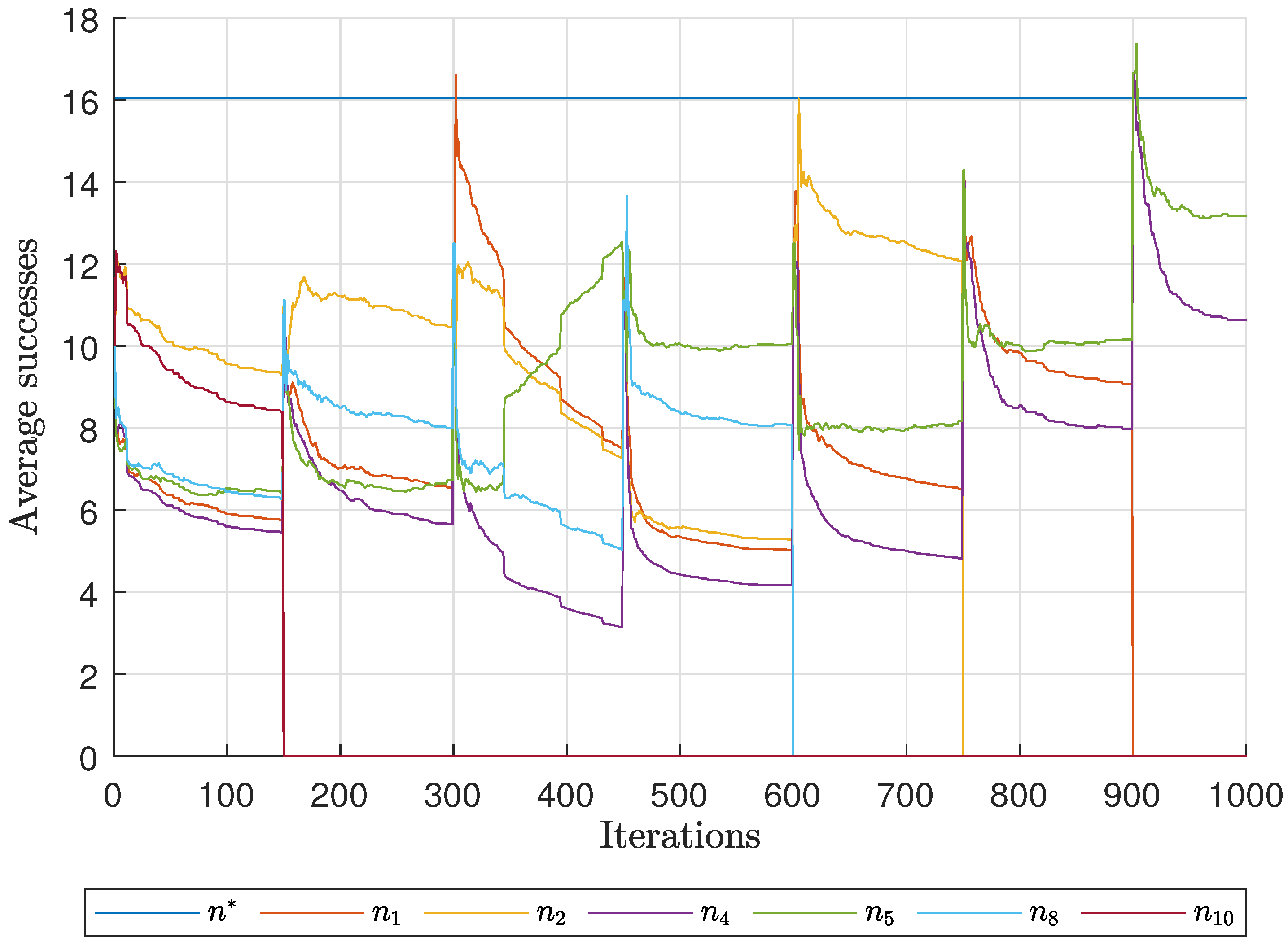
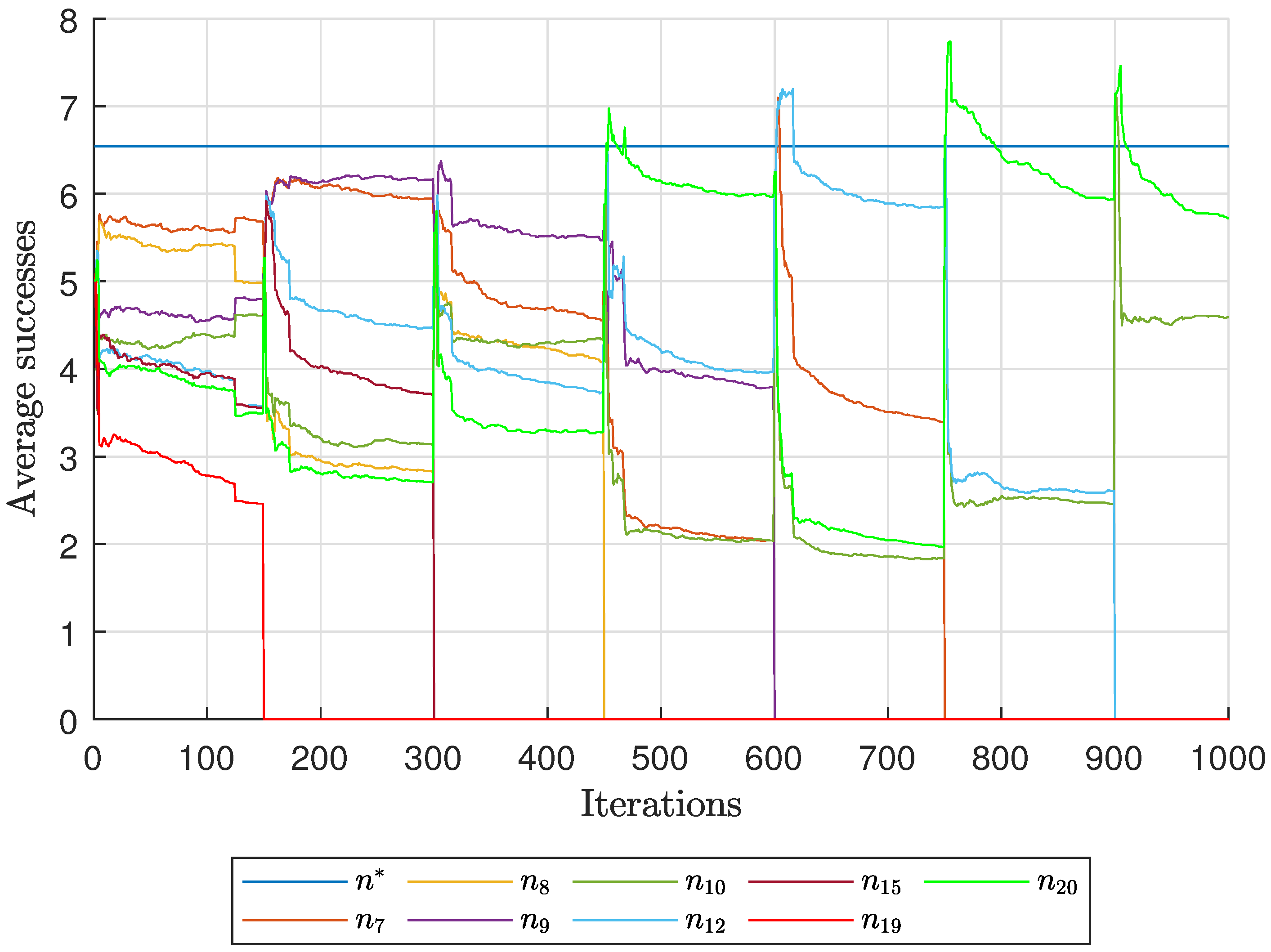
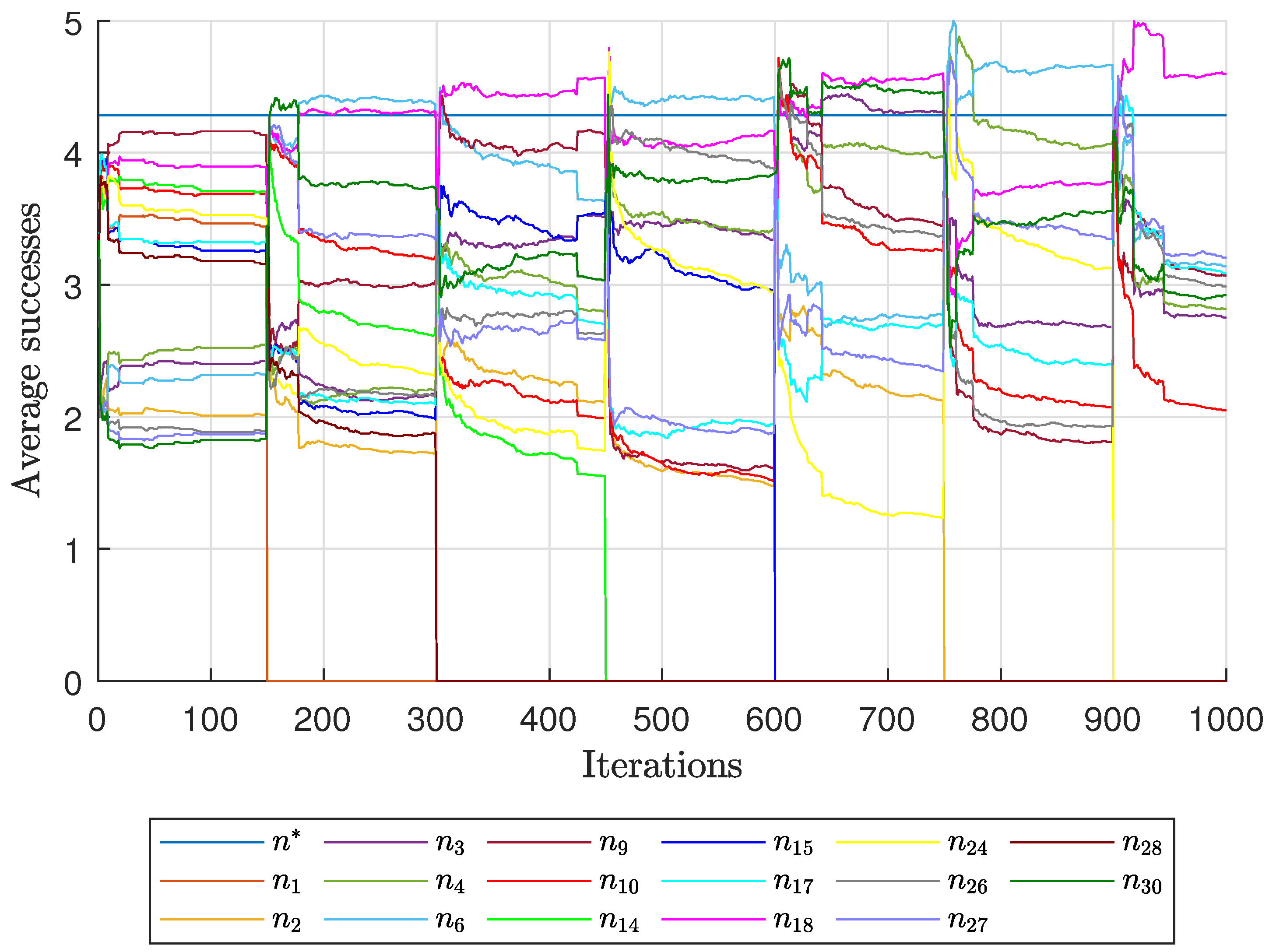
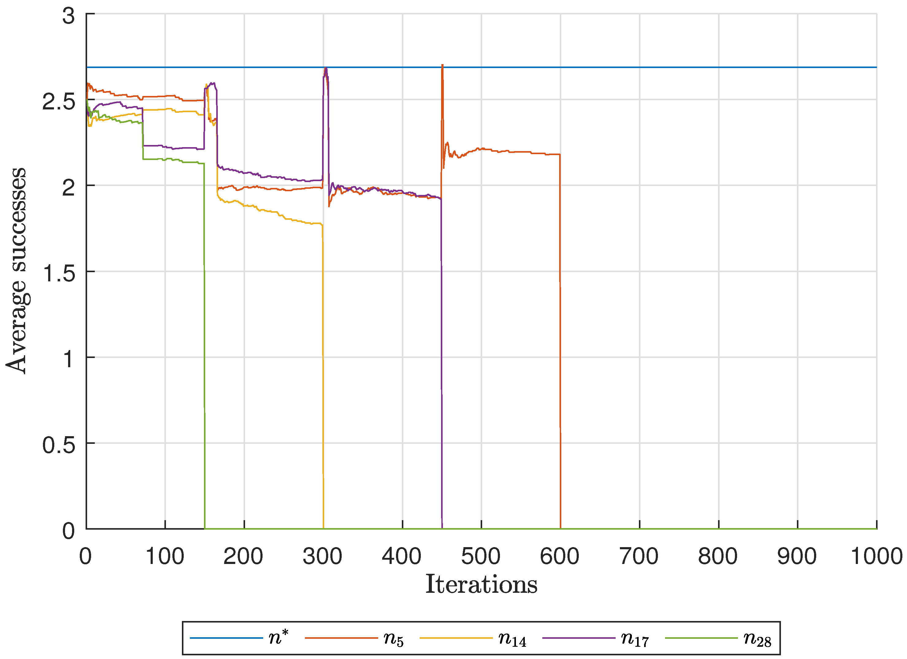
Diagnostic Visualization of the Node-Blocking Stage

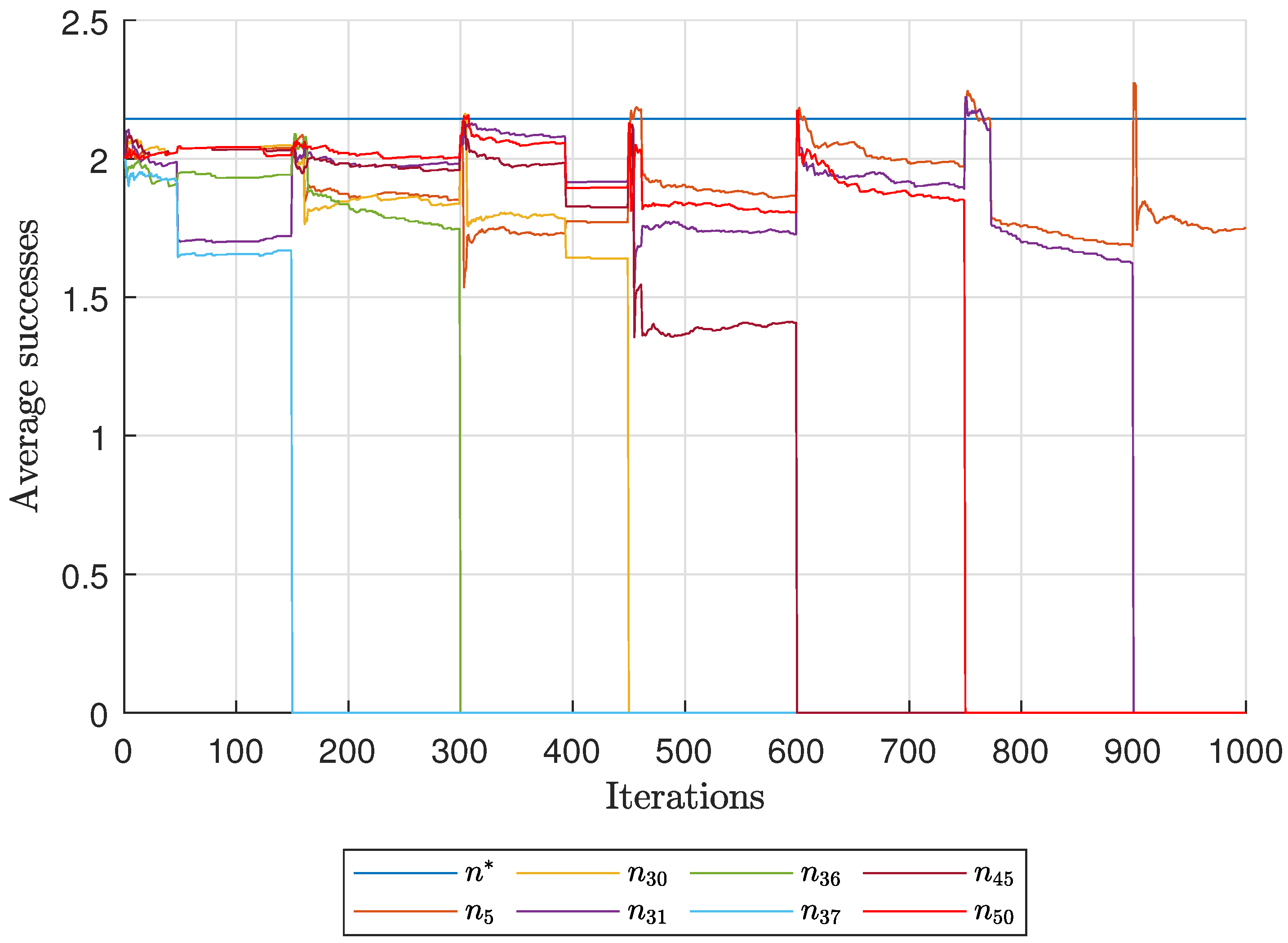
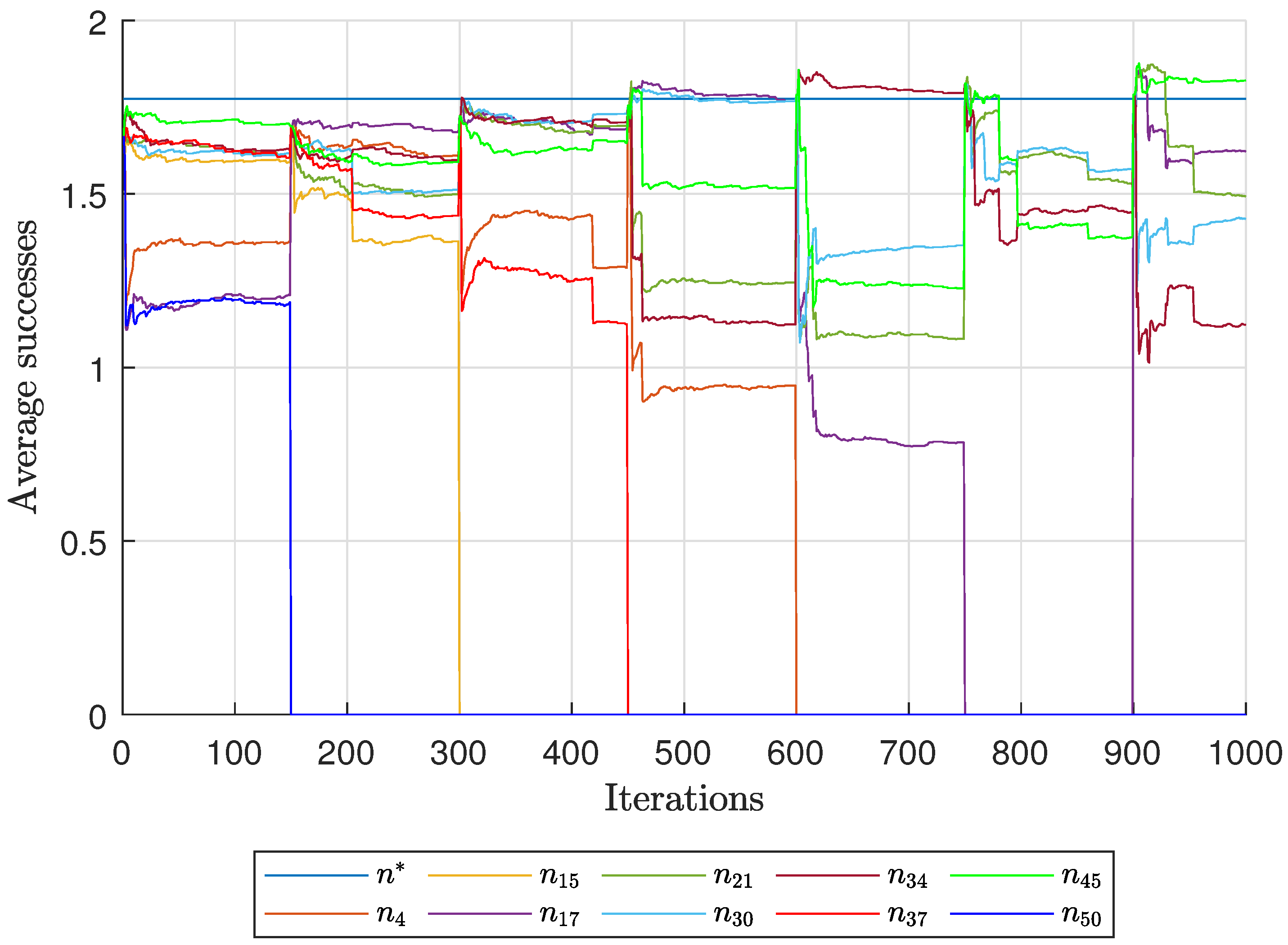
To illustrate the internal mechanics of the proposed blocking stage—biologically, how P. coffea wasps cease to visit unpromising nodes—we include the following diagnostic plots (Figure 17, Figure 18, Figure 19, Figure 20, Figure 21 and Figure 22). These figures are intended to explain how nodes are progressively blocked or excluded from the pinning set, rather than to provide additional performance benchmarks. For clarity, let $n^{*}$ denote the current average number of successful visits across the remaining (non-blocked) nodes; nodes below this running threshold are provisionally excluded from the pinning set, while blocked nodes become members of $\mathcal{B}\left(t\right)$. If stability is still not achieved after blocking or excluding a node, that node can be returned to the candidate pool, consistent with the update rules in Section 3.2.

As shown in Figure 17, the first network begins without any blocked nodes, but several nodes lie below the threshold. Figure 18 presents the corresponding behavior for Network 2, while Figure 19 illustrates a topology that requires fewer pinning nodes. Figure 20, Figure 21 and Figure 22 summarize the results for the remaining networks.

5. Conclusions

The proposed PHA-MD algorithm is an effective method for pinning control of complex networks, eliminating the need for prior information on the minimal number of pinned nodes. It is designed to solve multi-constraint optimization problems, focusing on optimal node selection with the minimal number of pinned nodes, while ensuring network stabilization through the V-stability tool.

A stability-first evaluation has been adopted. In the pinning control setting, feasibility (stability) is the primary objective; therefore, candidates that are energy-efficient but unstable are not considered valid solutions. Cross-method comparisons have been reported under equal population and iteration budgets and with explicit instability flags, so as not to conflate algorithmic merit with implementation details or with external enumeration required by fixed-dimension heuristics. Within this framing, PHA–MD consistently identified smaller, stable pinning sets and competitive energy levels across increasingly challenging network topologies.

A key advantage of PHA-MD is its ability to handle variable dimensions for its agents, unlike current algorithms that operate with fixed dimensions. This adaptability allows PHA-MD to address challenges related to permutations in pinning node selection, making it a robust and versatile solution for complex network control. Consequently, the hybrid nature of the optimization problem tackled by PHA-MD complicates direct comparisons with other collaborative behavior algorithms.

Future research could explore various weighting methodologies in penalty functions, analyze convergence times in border functions, and investigate more complex decision vector dynamics. These studies could further enhance the algorithm’s efficiency and applicability in more challenging scenarios, reinforcing its role as a leading solution in complex network control.