
Towards Full Forward On-Tiny-Device Learning: A Guided Search for a Randomly Initialized Neural Network


Abstract
1. Introduction
2. Problem Statement and Requirements
3. Related Works
3.1. Bayesian Optimization
3.2. Bayesian Optimization in Neural Architecture Search
3.3. Limits of Backpropagation
3.4. Extreme Learning Machines
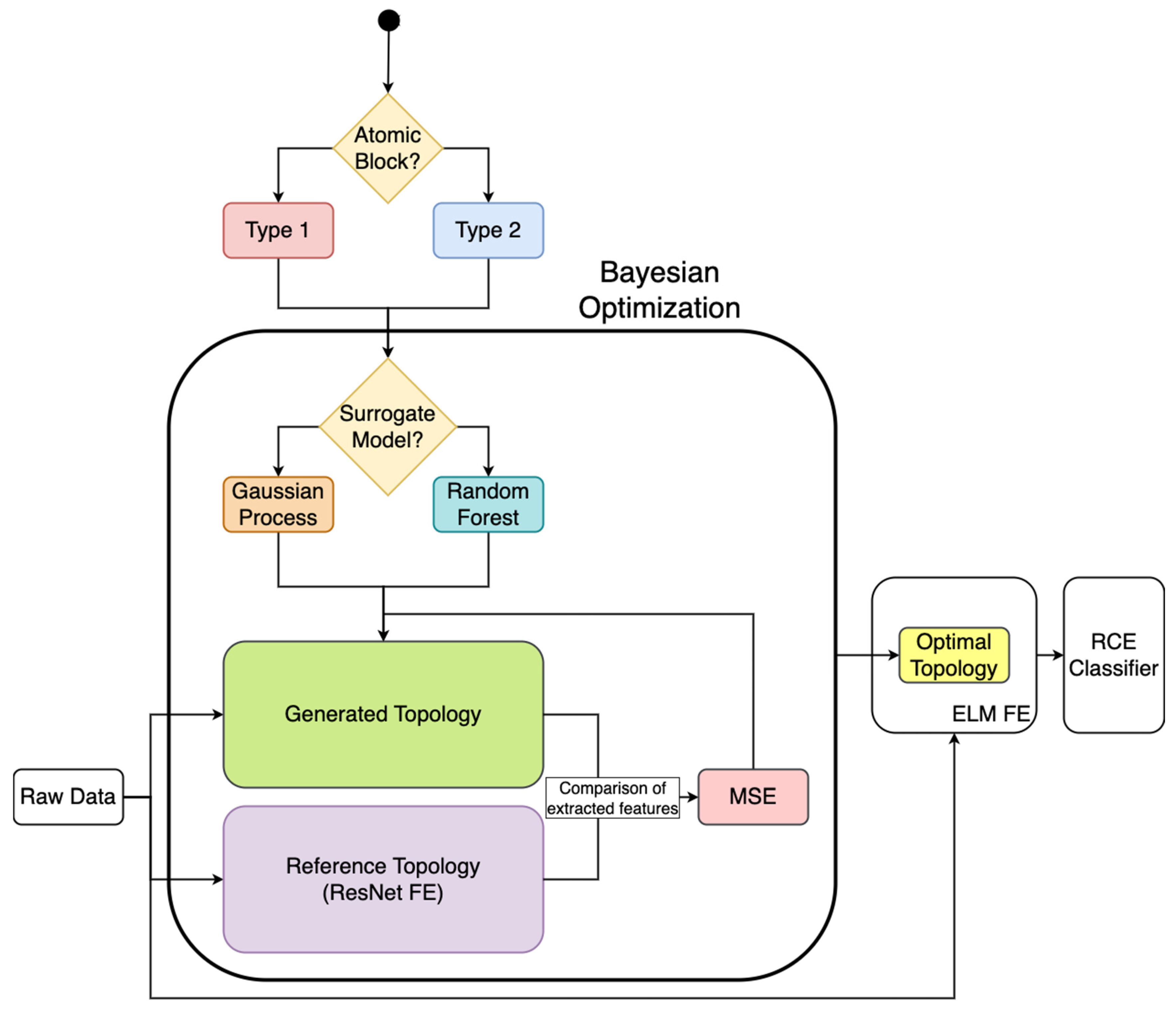
4. Materials and Methods
4.1. Datasets
4.2. Methodology
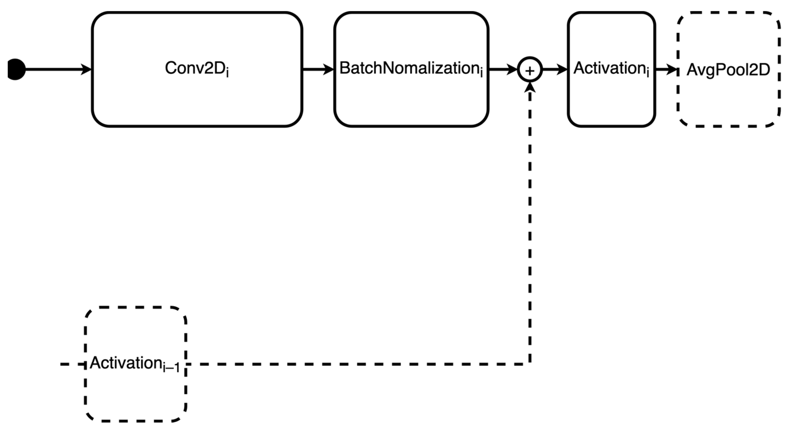
4.2.1. Definition of the Search Space
- Sum of residuals before activation layer: in this case, the topology does not include the possibility of summing the previous activation layer’s residual.
- Padding within the convolutional layers: for type 2 topologies, the ‘same’ padding is always applied.
4.2.2. Definition of the Search Strategy
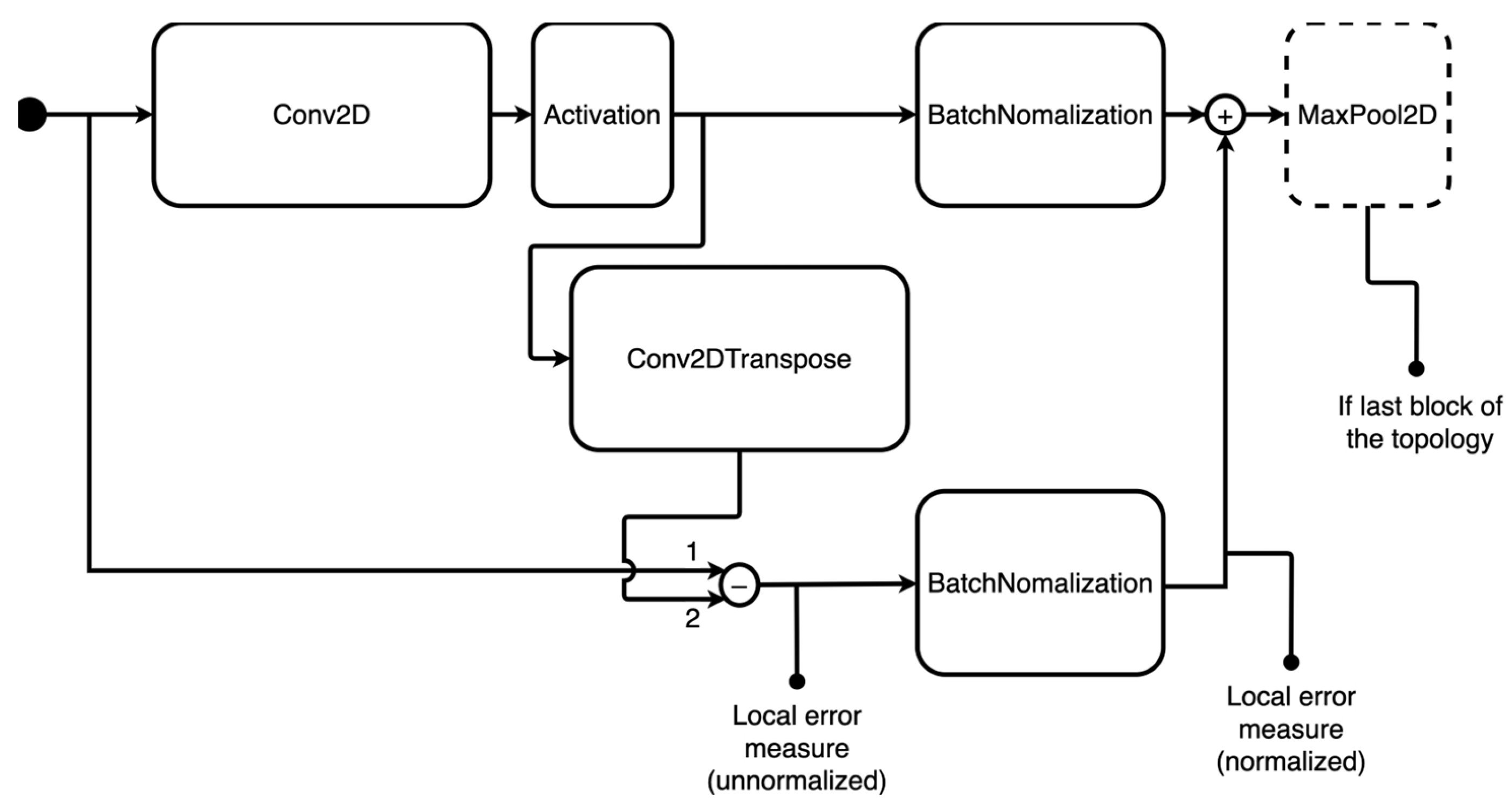
4.2.3. Definition of the Performance Estimation Strategy
5. Results
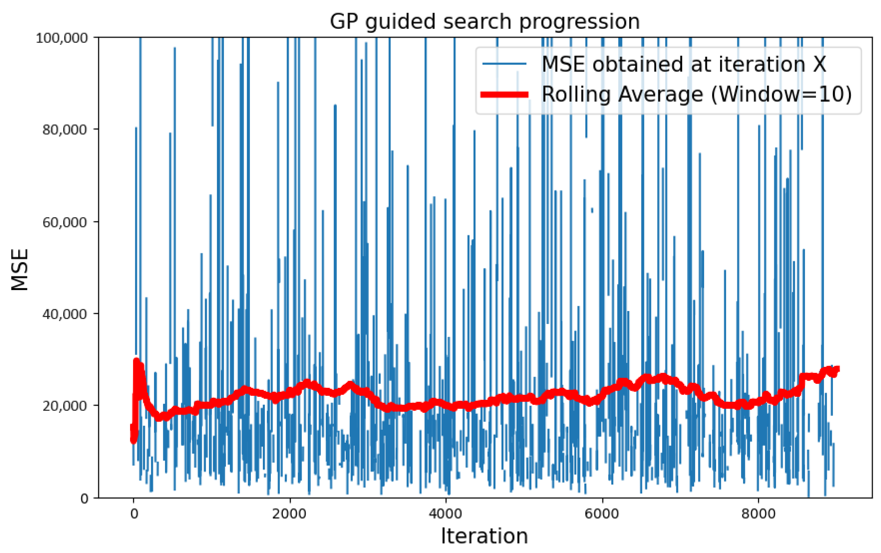
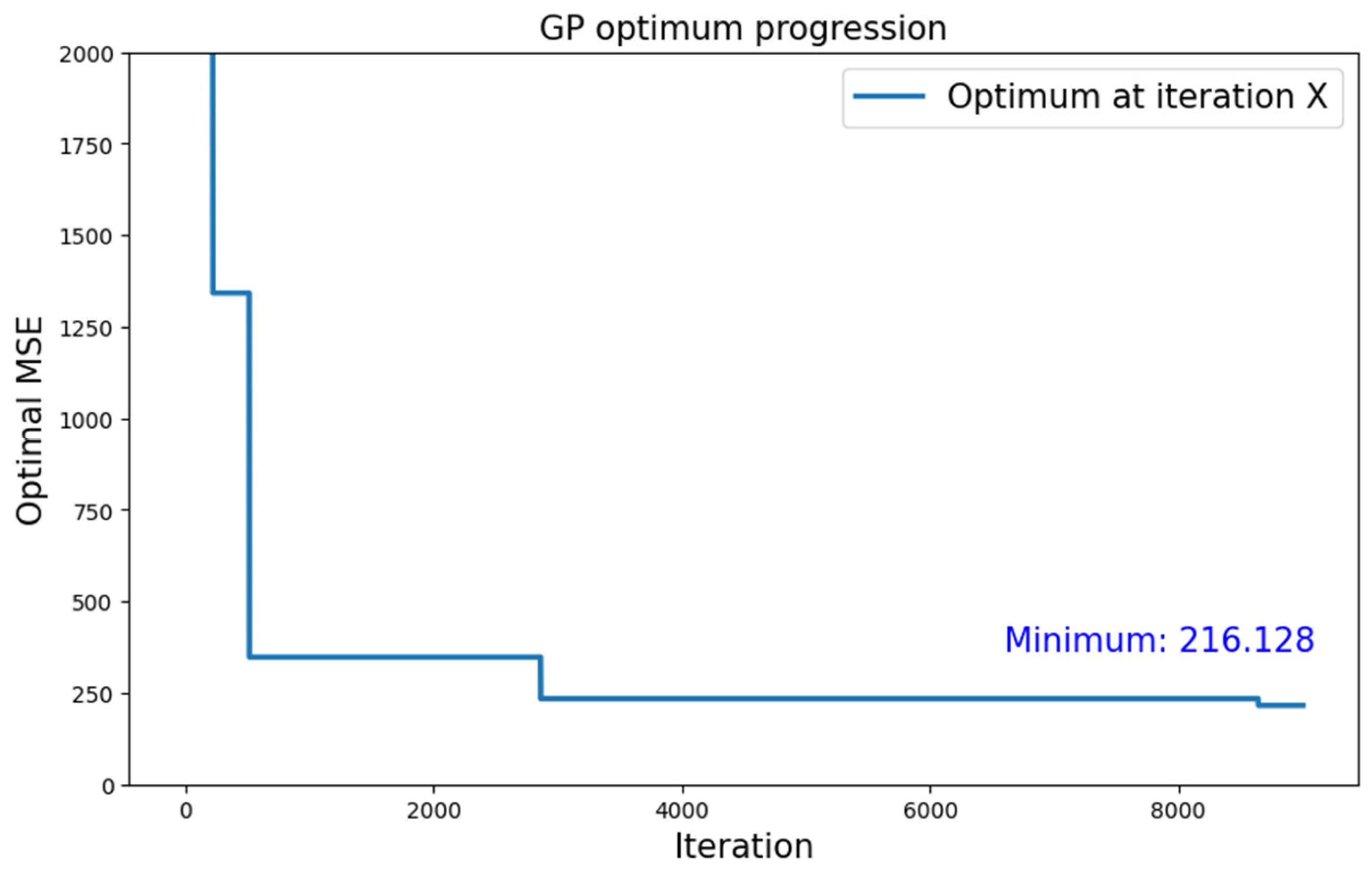
5.1. GP Surrogate Model with Type 1 Search Space
5.1.1. CIFAR-10 Dataset
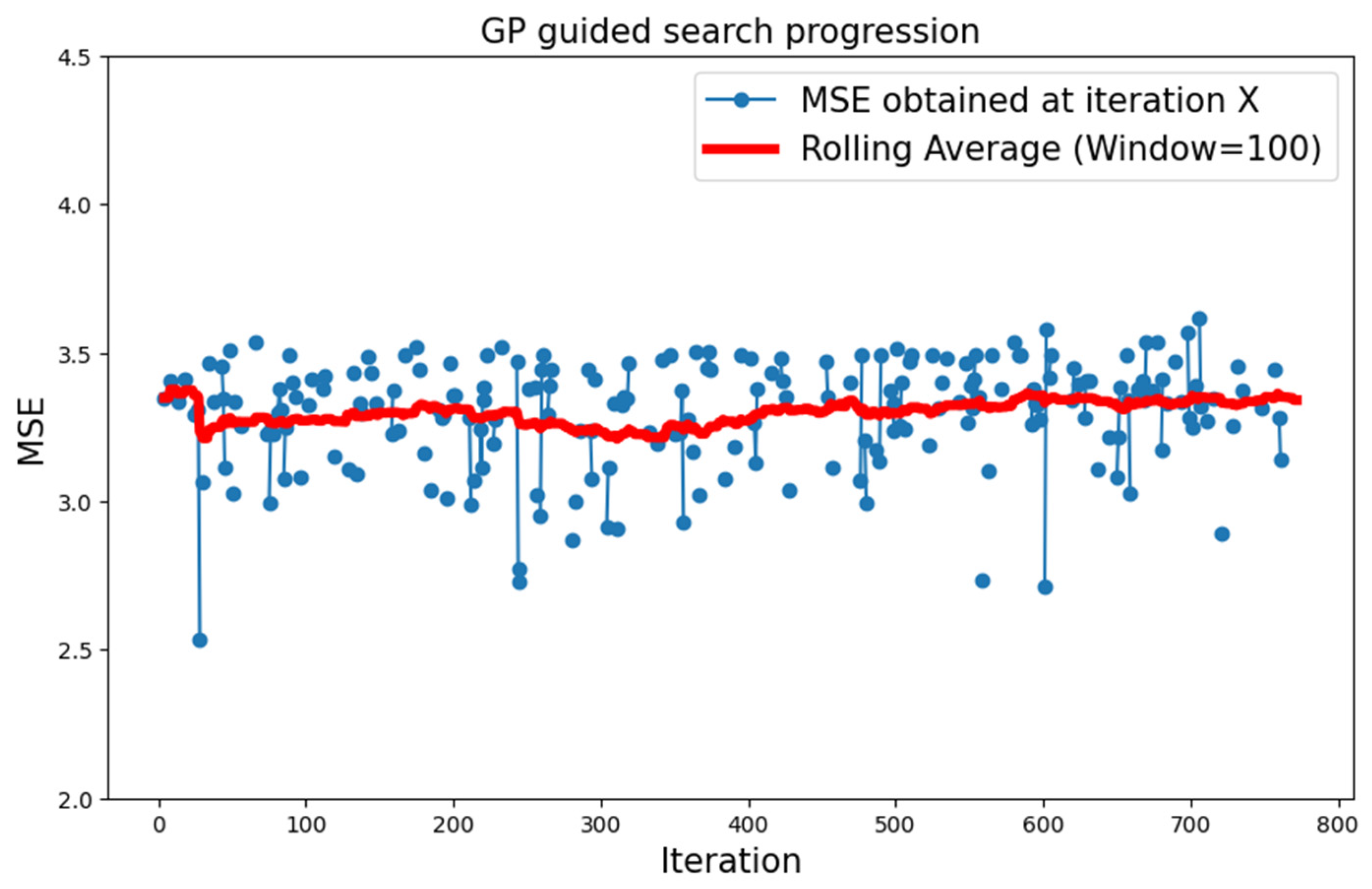
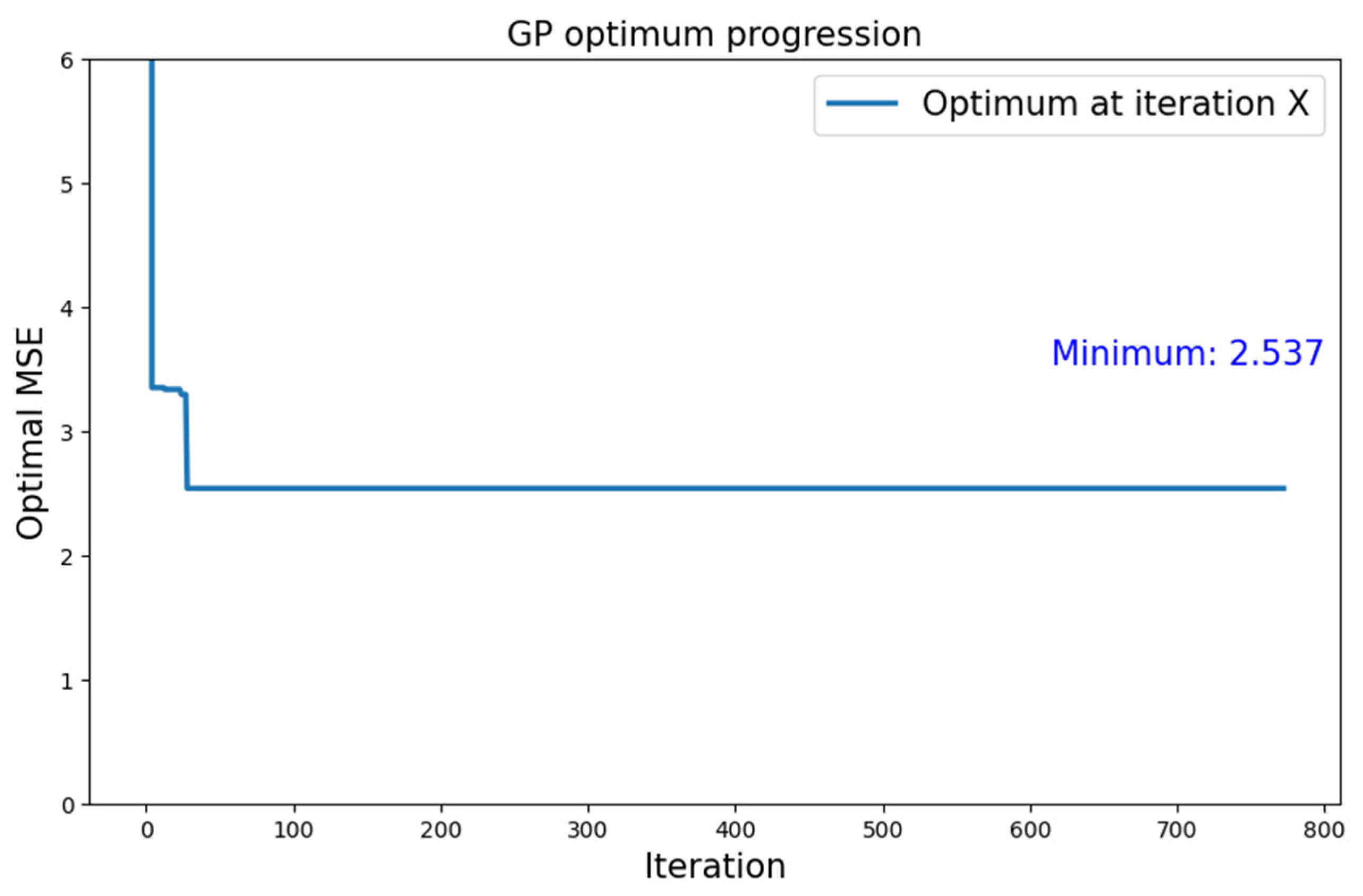
5.1.2. MNIST Dataset
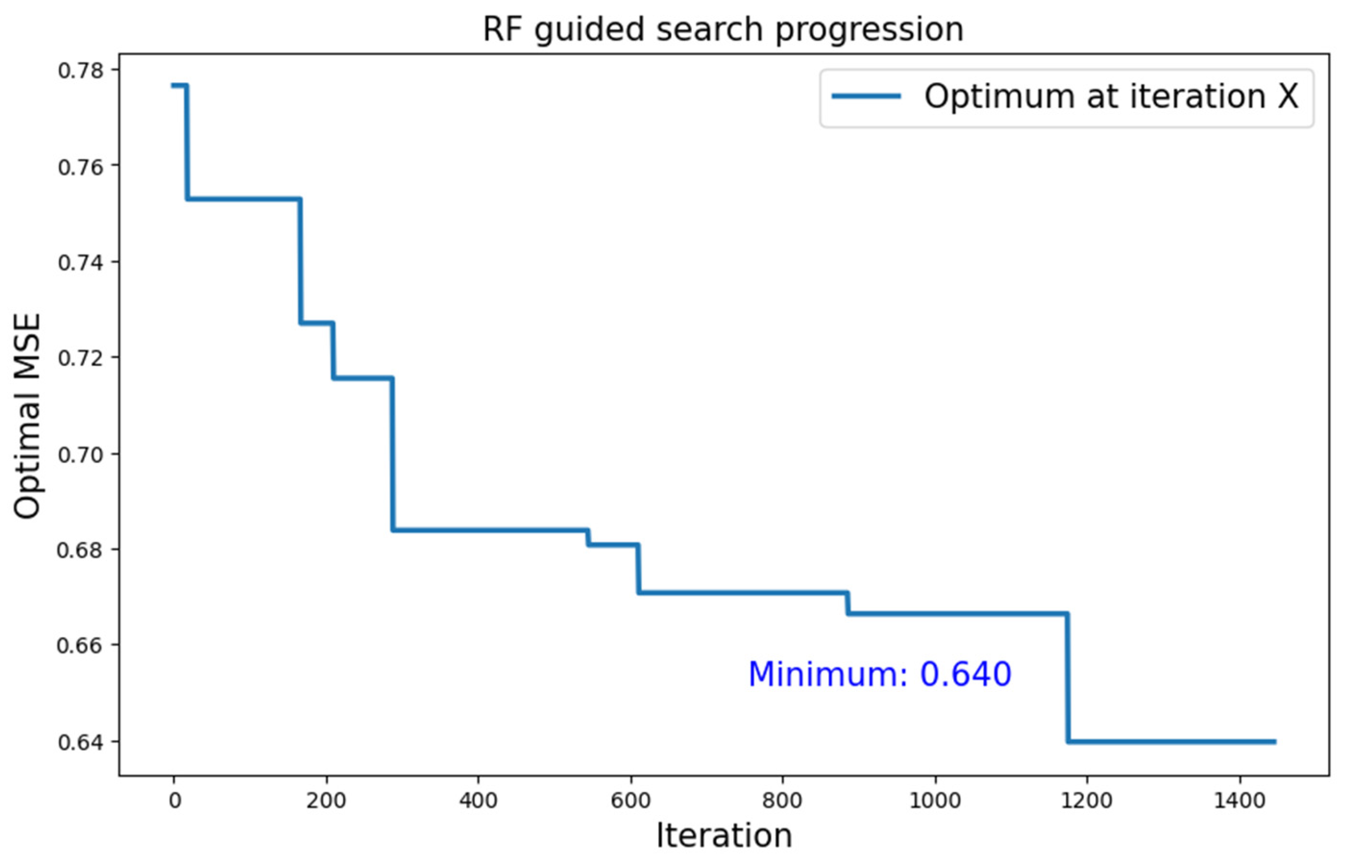
5.2. RF Surrogate Model with Type 1 Search Space
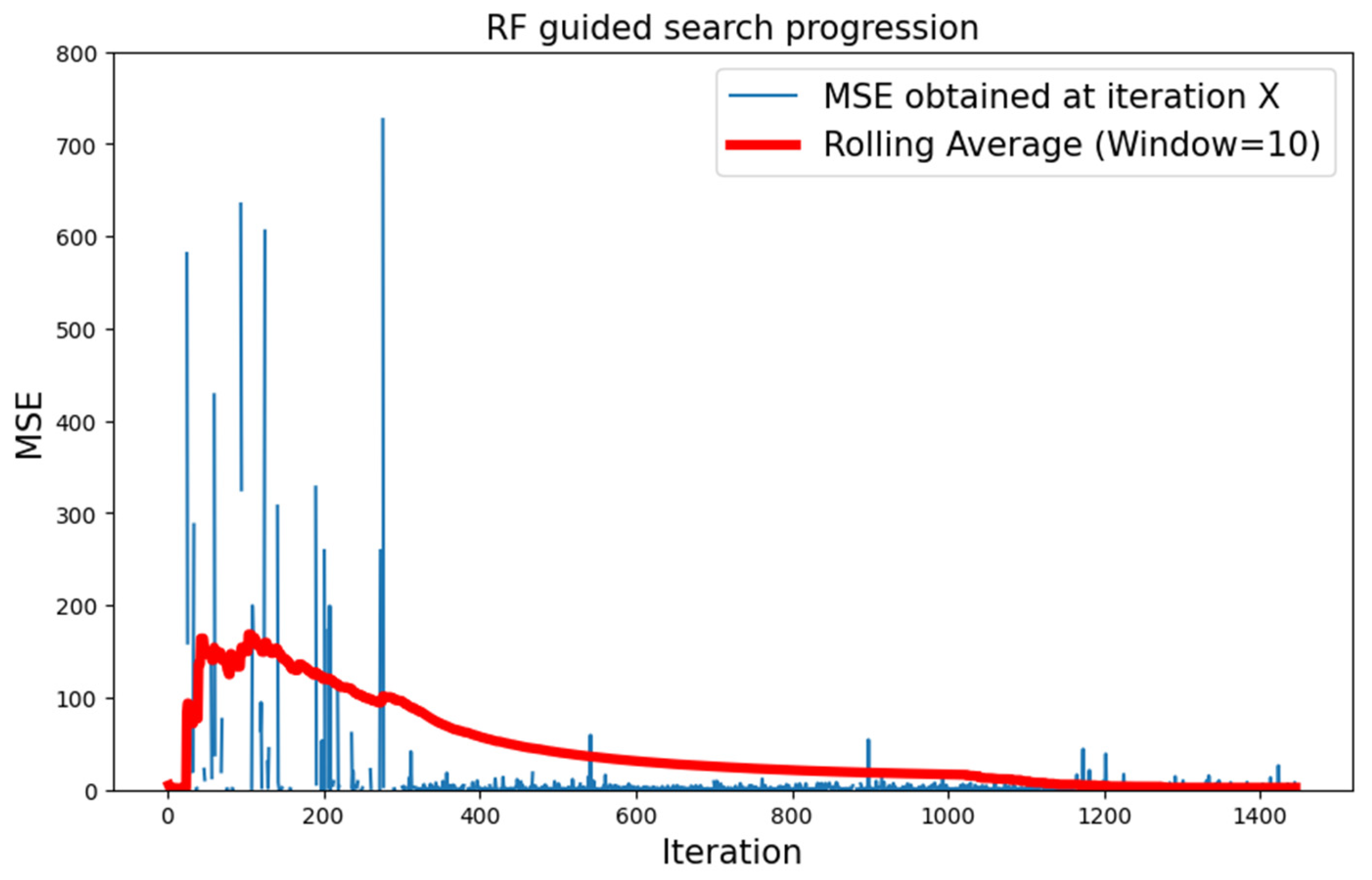
5.2.1. CIFAR-10 Dataset
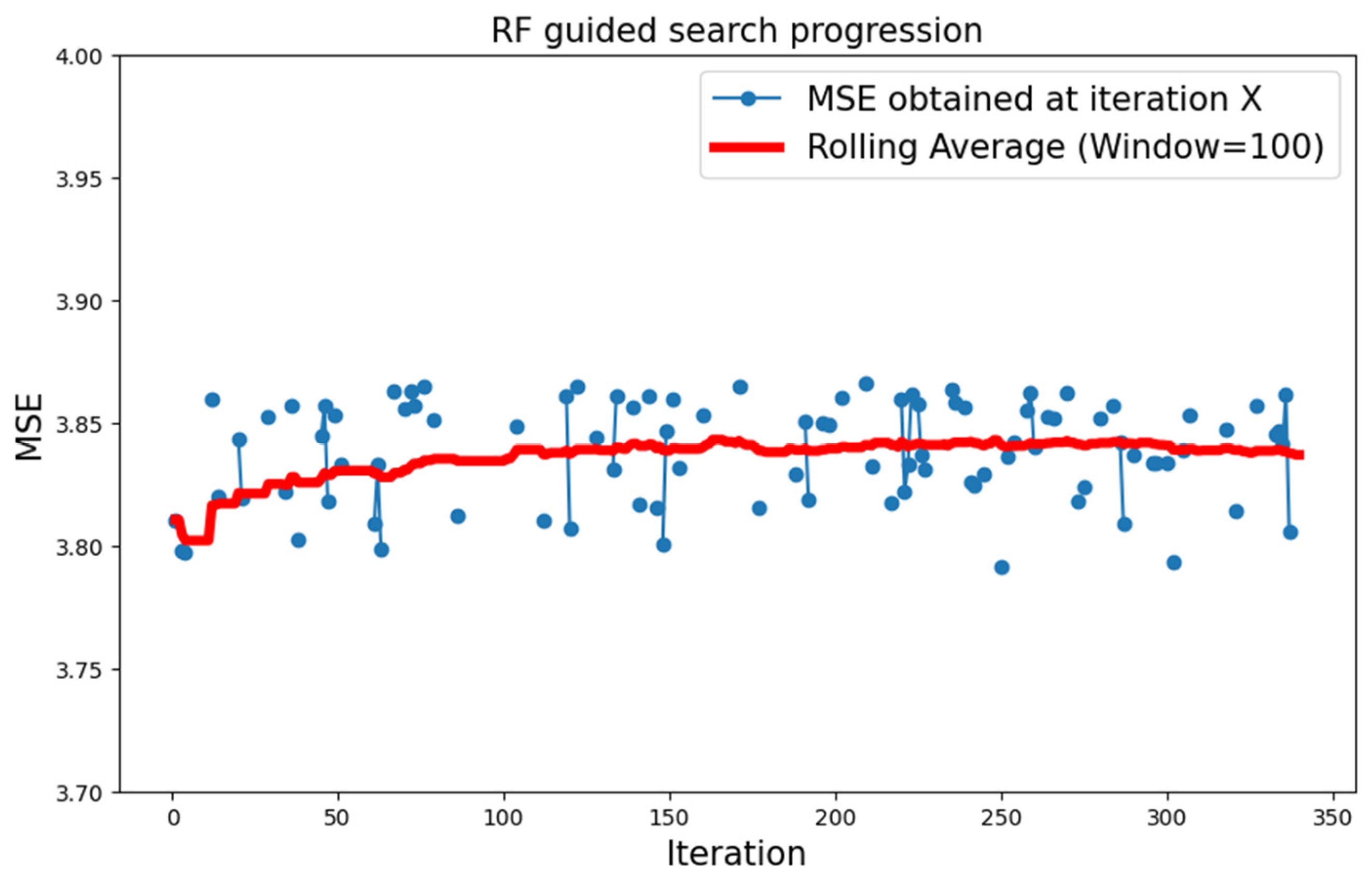
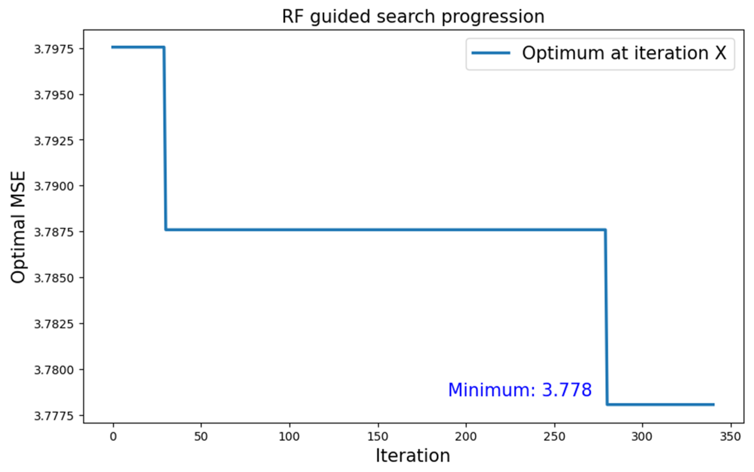
5.2.2. MNIST Dataset
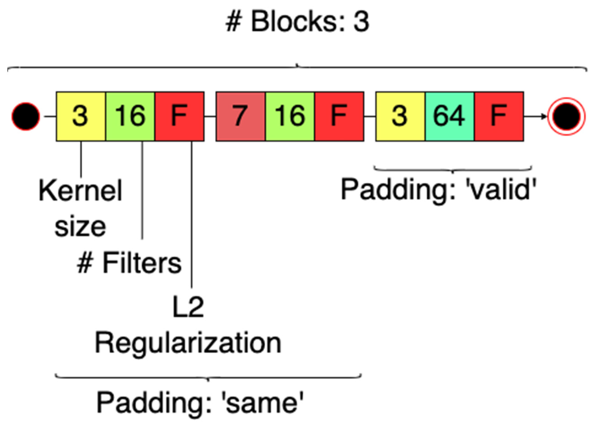
5.3. RF Surrogate Model with Type 2 Search Space
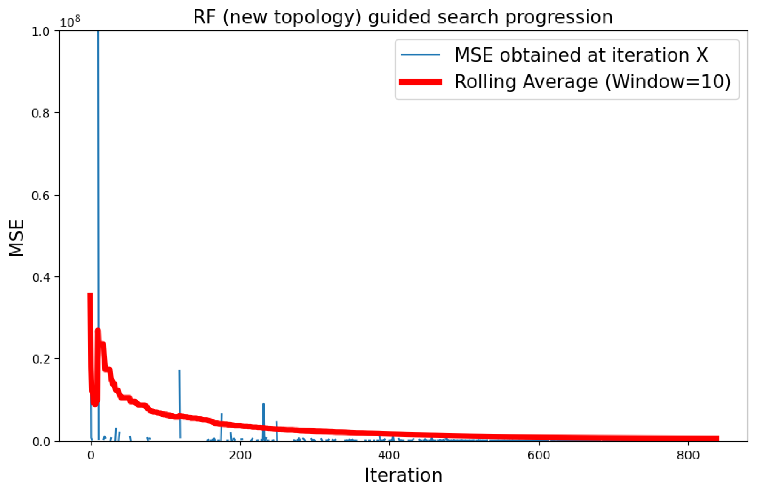
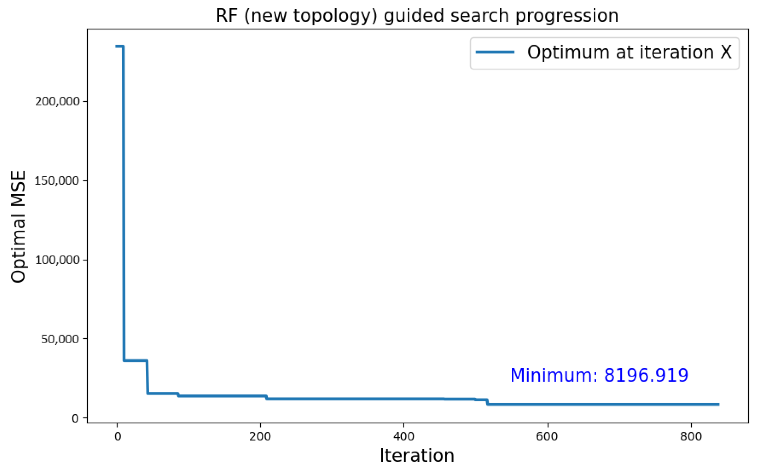
5.3.1. CIFAR-10 Dataset
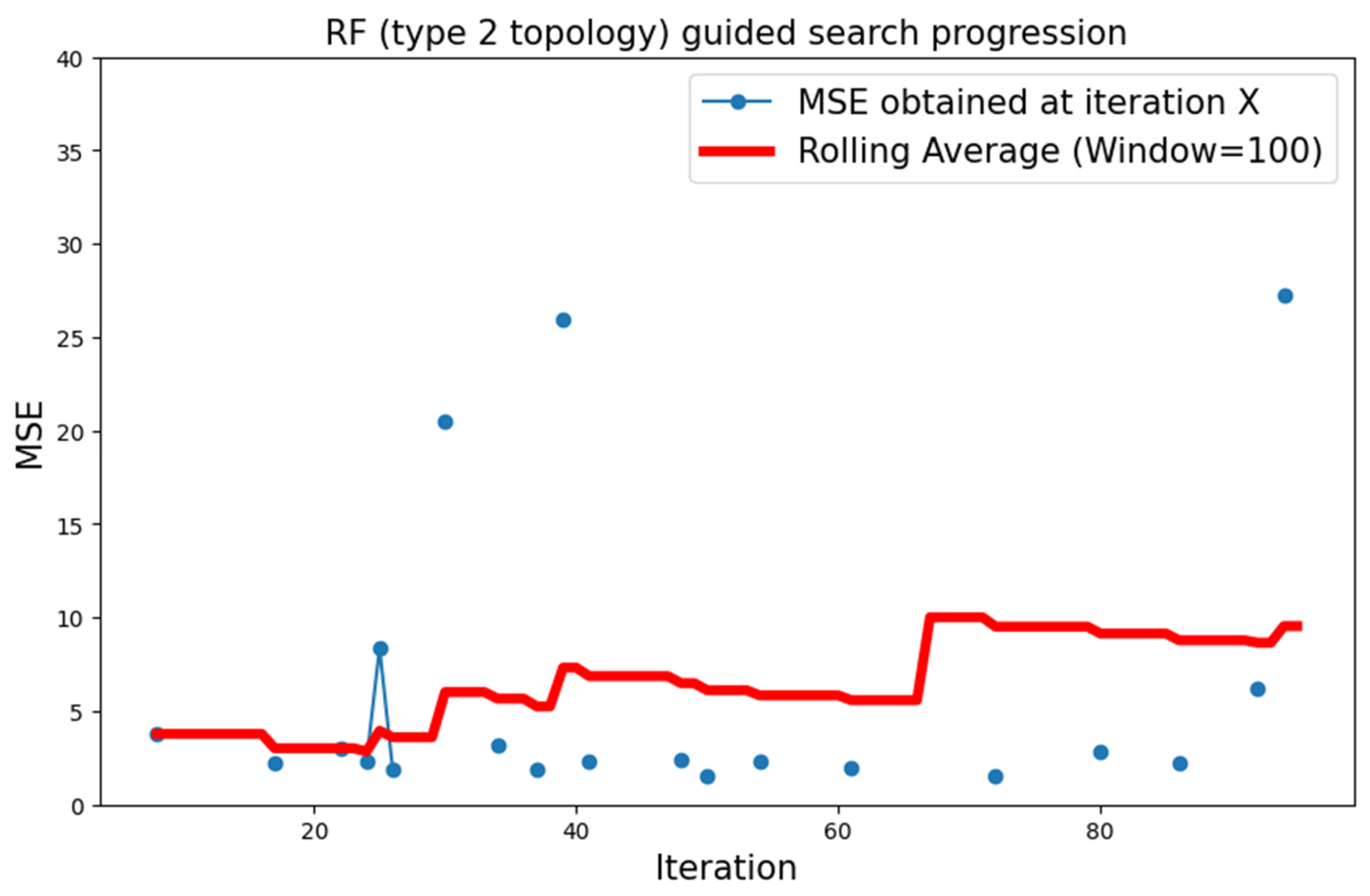
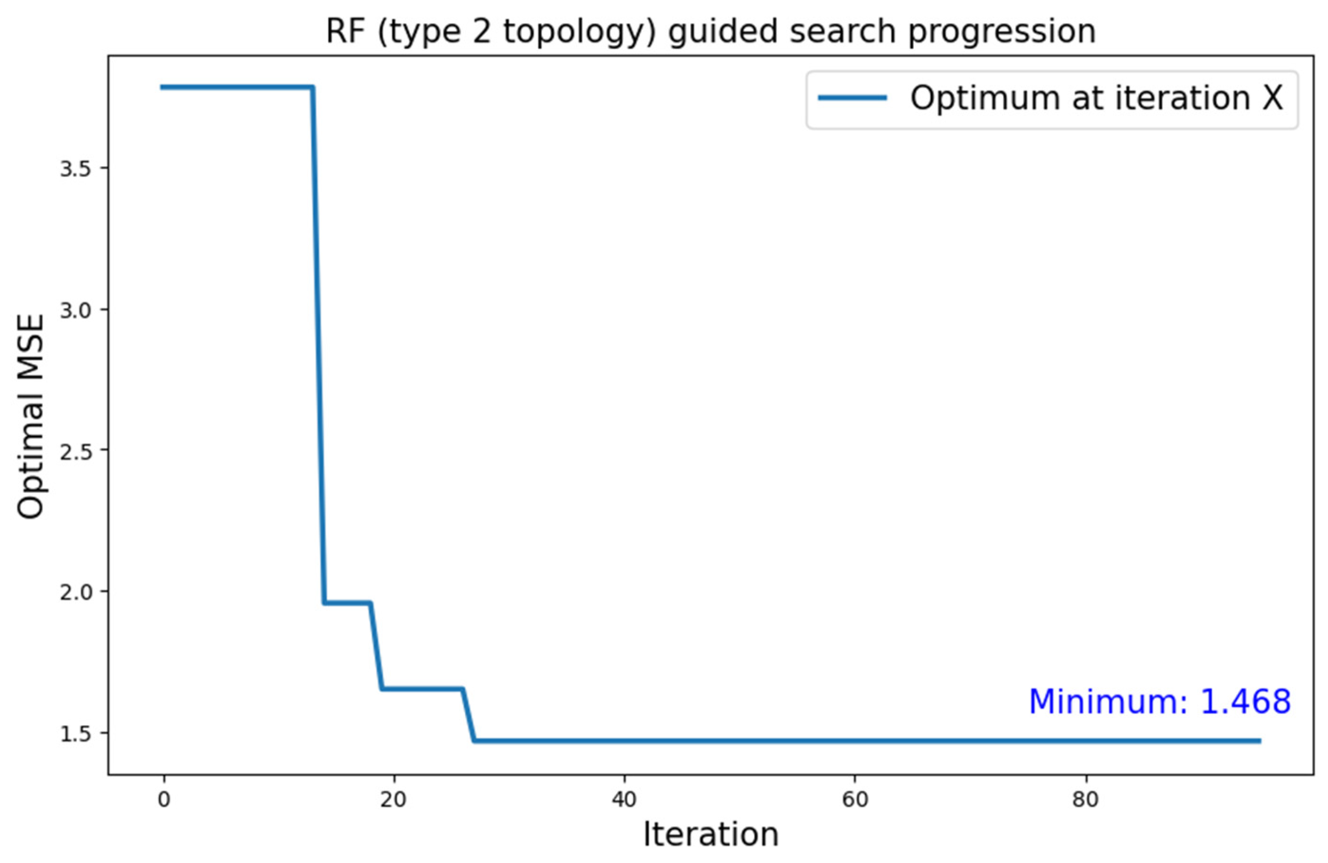
5.3.2. MNIST Dataset
5.4. Summary of the Results
6. Discussion and Conclusions
Author Contributions
Funding
Data Availability Statement
Conflicts of Interest
References
- Bianco, S.; Cadène, R.; Celona, L.; Napoletano, P. Benchmark Analysis of Representative Deep Neural Network Architectures. IEEE Access 2018, 6, 64270–64277. [Google Scholar] [CrossRef]
- Nagel, M.; Fournarakis, M.; Amjad, R.A.; Bondarenko, Y.; van Baalen, M.; Blankevoort, T. A White Paper on Neural Network Quantization. arXiv 2021, arXiv:2106.08295. [Google Scholar] [CrossRef]
- Li, H.; Kadav, A.; Durdanovic, I.; Samet, H.; Graf, H.P. Pruning Filters for Efficient ConvNets. arXiv 2016, arXiv:1608.08710. [Google Scholar] [CrossRef]
- Samie, F.; Bauer, L.; Henkel, J. From Cloud Down to Things: An Overview of Machine Learning in Internet of Things. IEEE Internet Things J. 2019, 6, 4921–4934. [Google Scholar] [CrossRef]
- Dhar, S.; Guo, J.; Liu, J.; Tripathi, S.; Kurup, U.; Shah, M. A Survey of On-Device Machine Learning: An Algorithms and Learning Theory Perspective. ACM Trans. Internet Things 2021, 2, 15. [Google Scholar] [CrossRef]
- O’Shea, K.; Nash, R. An Introduction to Convolutional Neural Networks. arXiv 2015, arXiv:1511.08458. [Google Scholar] [CrossRef]
- Cai, H.; Gan, C.; Zhu, L.; Han, S. TinyTL: Reduce Memory, Not Parameters for Efficient on-Device Learning. In Advances in Neural Information Processing Systems; Larochelle, H., Ranzato, M., Hadsell, R., Balcan, M.F., Lin, H., Eds.; Curran Associates, Inc.: Red Hook, NY, USA, 2020; Volume 33, pp. 11285–11297. [Google Scholar]
- Lin, J.; Zhu, L.; Chen, W.-M.; Wang, W.-C.; Gan, C.; Han, S. On-Device Training under 256kb Memory. arXiv 2022, arXiv:2206.15472. [Google Scholar]
- Huang, G.-B.; Zhu, Q.-Y.; Siew, C.K. Extreme Learning Machine: Theory and Applications. Neurocomputing 2006, 70, 489–501. [Google Scholar] [CrossRef]
- Wang, J.; Lu, S.; Wang, S.; Zhang, Y. A Review on Extreme Learning Machine. Multimed. Tools Appl. 2021, 81, 41611–41660. [Google Scholar] [CrossRef]
- Bull, D.R.; Zhang, F. Digital Picture Formats and Representations. In Intelligent Image and Video Compression; Elsevier: Amsterdam, The Netherlands, 2021; pp. 107–142. ISBN 978-0-12-820353-8. [Google Scholar]
- Bosse, S.; Maniry, D.; Wiegand, T.; Samek, W. A Deep Neural Network for Image Quality Assessment. In Proceedings of the 2016 IEEE International Conference on Image Processing (ICIP), Phoenix, AZ, USA, 25–28 September 2016; pp. 3773–3777. [Google Scholar]
- Ding, K.; Liu, Y.; Zou, X.; Wang, S.; Ma, K. Locally Adaptive Structure and Texture Similarity for Image Quality Assessment. In Proceedings of the 29th ACM International Conference on Multimedia, Virtual, 17 October 2021; pp. 2483–2491. [Google Scholar]
- Garnett, R. Bayesian Optimization; Cambridge University Press: Cambridge, UK; New York, NY, USA, 2023; ISBN 978-1-108-42578-0. [Google Scholar]
- Candelieri, A. A Gentle Introduction to Bayesian Optimization. In Proceedings of the 2021 Winter Simulation Conference (WSC), Phoenix, AZ, USA, 12 December 2021; pp. 1–16. [Google Scholar]
- Archetti, F.; Candelieri, A. Bayesian Optimization and Data Science; SpringerBriefs in Optimization; Springer International Publishing: Cham, Switzerland, 2019; ISBN 978-3-030-24493-4. [Google Scholar]
- Frazier, P.I. Bayesian Optimization. In Recent Advances in Optimization and Modeling of Contemporary Problems; Gel, E., Ntaimo, L., Shier, D., Greenberg, H.J., Eds.; INFORMS: Catonsville, MD, USA, 2018; pp. 255–278. ISBN 978-0-9906153-2-3. [Google Scholar]
- Guyon, I.; Sun-Hosoya, L.; Boullé, M.; Escalante, H.J.; Escalera, S.; Liu, Z.; Jajetic, D.; Ray, B.; Saeed, M.; Sebag, M.; et al. Analysis of the AutoML Challenge Series 2015–2018. In Automated Machine Learning; Springer: Berlin/Heidelberg, Germany, 2019. [Google Scholar]
- Perego, R.; Candelieri, A.; Archetti, F.; Pau, D. AutoTinyML for Microcontrollers: Dealing with Black-Box Deployability. Expert Syst. Appl. 2022, 207, 117876. [Google Scholar] [CrossRef]
- Močkus, J. On Bayesian Methods for Seeking the Extremum. In Optimization Techniques IFIP Technical Conference Novosibirsk, July 1–7, 1974; Marchuk, G.I., Ed.; Lecture Notes in Computer Science; Springer: Berlin/Heidelberg, Germany, 1975; Volume 27, pp. 400–404. ISBN 978-3-540-07165-5. [Google Scholar]
- Mockus, J. Bayesian Approach to Global Optimization: Theory and Applications; Mathematics and its applications, Soviet series; Kluwer Academic: Dordrecht, The Netherlands; Boston, MA, USA, 1989; ISBN 978-0-7923-0115-8. [Google Scholar]
- Berger, J.O. Statistical Decision Theory. In Time Series and Statistics; Eatwell, J., Milgate, M., Newman, P., Eds.; Palgrave Macmillan: London, UK, 1990; pp. 277–284. ISBN 978-0-333-49551-3. [Google Scholar]
- Breiman, L. Random Forests. Mach. Learn. 2001, 45, 5–32. [Google Scholar] [CrossRef]
- Hutter, F.; Hoos, H.H.; Leyton-Brown, K. Sequential Model-Based Optimization for General Algorithm Configuration. In Learning and Intelligent Optimization; Coello, C.A.C., Ed.; Lecture Notes in Computer Science; Springer: Berlin/Heidelberg, Germany, 2011; Volume 6683, pp. 507–523. ISBN 978-3-642-25565-6. [Google Scholar]
- Wang, X.; Jin, Y.; Schmitt, S.; Olhofer, M. Recent Advances in Bayesian Optimization. ACM Comput. Surv. 2023, 55, 287. [Google Scholar] [CrossRef]
- Wistuba, M.; Wistuba, M.; Rawat, A.; Pedapati, T. A Survey on Neural Architecture Search. arXiv 2019, arXiv:1905.01392. [Google Scholar]
- Van Son, D.; De Putter, F.; Vogel, S.; Corporaal, H. BOMP-NAS: Bayesian Optimization Mixed Precision NAS. In Proceedings of the 2023 Design, Automation & Test in Europe Conference & Exhibition (DATE), Antwerp, Belgium, 17–19 April 2023; pp. 1–2. [Google Scholar]
- White, C.; Neiswanger, W.; Savani, Y. BANANAS: Bayesian Optimization with Neural Architectures for Neural Architecture Search. Proc. AAAI Conf. Artif. Intell. 2021, 35, 10293–10301. [Google Scholar] [CrossRef]
- Shen, Y.; Li, Y.; Zheng, J.; Zhang, W.; Yao, P.; Li, J.; Yang, S.; Liu, J.; Cui, B. ProxyBO: Accelerating Neural Architecture Search via Bayesian Optimization with Zero-Cost Proxies. Proc. AAAI Conf. Artif. Intell. 2023, 37, 9792–9801. [Google Scholar] [CrossRef]
- Jiang, Y.; Yang, F.; Yu, B.; Zhou, D.; Zeng, X. Efficient Layout Hotspot Detection via Neural Architecture Search. ACM Trans. Des. Autom. Electron. Syst. 2022, 27, 62. [Google Scholar] [CrossRef]
- Yang, Z.; Zhang, S.; Li, R.; Li, C.; Wang, M.; Wang, D.; Zhang, M. Efficient Resource-Aware Convolutional Neural Architecture Search for Edge Computing with Pareto-Bayesian Optimization. Sensors 2021, 21, 444. [Google Scholar] [CrossRef]
- Elsken, T.; Metzen, J.H.; Hutter, F. Neural Architecture Search: A Survey. J. Mach. Learn. Res. 2019, 20, 1997–2017. [Google Scholar]
- Capogrosso, L.; Cunico, F.; Cheng, D.S.; Fummi, F.; Cristani, M. A Machine Learning-Oriented Survey on Tiny Machine Learning. arXiv 2023, arXiv:2309.11932. [Google Scholar] [CrossRef]
- Gong, Y.; Liu, L.; Yang, M.; Bourdev, L. Compressing Deep Convolutional Networks Using Vector Quantization. ArXiv Comput. Vis. Pattern Recognit. 2014, arXiv:1412.6115. [Google Scholar]
- Han, S.; Mao, H.; Dally, W.J. Deep Compression: Compressing Deep Neural Networks with Pruning, Trained Quantization and Huffman Coding. ArXiv Comput. Vis. Pattern Recognit. 2015, arXiv:1510.00149. [Google Scholar]
- Hinton, G.E.; Vinyals, O.; Dean, J. Distilling the Knowledge in a Neural Network. ArXiv Mach. Learn. 2015, arXiv:1503.02531. [Google Scholar]
- Cho, J.H.; Hariharan, B. On the Efficacy of Knowledge Distillation. In Proceedings of the IEEE/CVF International Conference on Computer Vision (ICCV), Seoul, Repulic of Korea, 27 October–2 November 2019. [Google Scholar]
- Deng, B.L.; Li, G.; Han, S.; Shi, L.; Xie, Y. Model Compression and Hardware Acceleration for Neural Networks: A Comprehensive Survey. Proc. IEEE 2020, 108, 485–532. [Google Scholar] [CrossRef]
- Ghimire, D.; Kil, D.; Kim, S. A Survey on Efficient Convolutional Neural Networks and Hardware Acceleration. Electronics 2022, 11, 945. [Google Scholar] [CrossRef]
- Lillicrap, T.P.; Santoro, A.; Marris, L.; Akerman, C.J.; Hinton, G. Backpropagation and the Brain. Nat. Rev. Neurosci. 2020, 21, 335–346. [Google Scholar] [CrossRef] [PubMed]
- Huang, G.-B.; Liang, N.-Y.; Liang, N.; Wong, P.K.; Rong, H.-J.; Saratchandran, P.; Sundararajan, N. On-Line Sequential Extreme Learning Machine. In Proceedings of the IASTED International Conference on Computational Intelligence, Calgary, AB, Canada, 4–6 July 2005; pp. 232–237. [Google Scholar]
- Huang, G.-B. Reply to “Comments on ‘The Extreme Learning Machine”. IEEE Trans. Neural Netw. 2008, 19, 1495–1496. [Google Scholar] [CrossRef]
- Huang, G.-B.; Zhou, H.; Ding, X.; Zhang, R.; Zhang, R. Extreme Learning Machine for Regression and Multiclass Classification. IEEE Trans. Syst. Man Cybern. Part B Cybern. 2012, 42, 513–529. [Google Scholar] [CrossRef] [PubMed]
- Cambria, E.; Huang, G.-B.; Kasun, L.L.C.; Zhou, H.; Vong, C.-M.; Lin, J.; Yin, J.; Cai, Z.; Liu, Q.; Li, K.; et al. Extreme Learning Machine. IEEE Intell. Syst. 2013, 28, 30–59. [Google Scholar] [CrossRef]
- Huang, G.-B. What Are Extreme Learning Machines? Filling the Gap between Frank Rosenblatt’s Dream and John von Neumann’s Puzzle. Cogn. Comput. 2015, 7, 263–278. [Google Scholar] [CrossRef]
- CIFAR-10 and CIFAR-100 Datasets. Available online: http://www.cs.toronto.edu/~kriz/cifar.html (accessed on 7 March 2023).
- Banbury, C.; Reddi, V.J.; Torelli, P.; Jeffries, N.; Kiraly, C.; Holleman, J.; Montino, P.; Kanter, D.; Warden, P.; Pau, D.; et al. MLPerf Tiny Benchmark. NeurIPS Datasets Benchmarks 2021, 1. Available online: https://datasets-benchmarks-proceedings.neurips.cc/paper_files/paper/2021/file/da4fb5c6e93e74d3df8527599fa62642-Paper-round1.pdf (accessed on 4 May 2023).
- LeCun, Y. The MNIST Database of Handwritten Digits. 1998. Available online: http://yann.lecun.com/exdb/mnist/ (accessed on 23 October 2023).
- He, K.; Zhang, X.; Ren, S.; Sun, J. Deep Residual Learning for Image Recognition. arXiv 2015, arXiv:1512.03385. [Google Scholar]
- Pau, D.P.; Pisani, A.; Aymone, F.M.; Ferrari, G. TinyRCE: Multipurpose Forward Learning for Resource Restricted Devices. IEEE Sens. Lett. 2023, 7, 5503104. [Google Scholar] [CrossRef]


| Codename | Requirement |
|---|---|
| R1 | The proposed solution shall search and design an ELM CNN FE type topology. |
| R2 | The devised ELM CNN FE shall generate features that can be compared with those of a reference CNN which had been previously trained with backpropagation on a given dataset. |
| R3 | The mean square error between the features mentioned in R2 shall be less than or equal to one. |
| R4 | The proposed solution shall employ BO. |
| R5 | The proposed solution shall test at least two surrogate functions. |
| R6 | The proposed solution shall be tested on at least two network topology spaces. |
| Scope | Variable | Data Type | Search Bounds |
|---|---|---|---|
| Whole network | Number of blocks | Integer | (1, …, 10) |
| Whole network | Sum of residuals before Activation layer | Boolean | (True, False) |
| Convolutional layer | Padding type | Categorical | (‘valid’, ‘same’) |
| Convolutional layer | Kernel size | Integer | (3, 5, 7) |
| Convolutional layer | Number of filters | Integer | (16, 32, 64) |
| Convolutional layer | L2 Regularization | Boolean | (True, False) |
| Scope | Variable | Values |
|---|---|---|
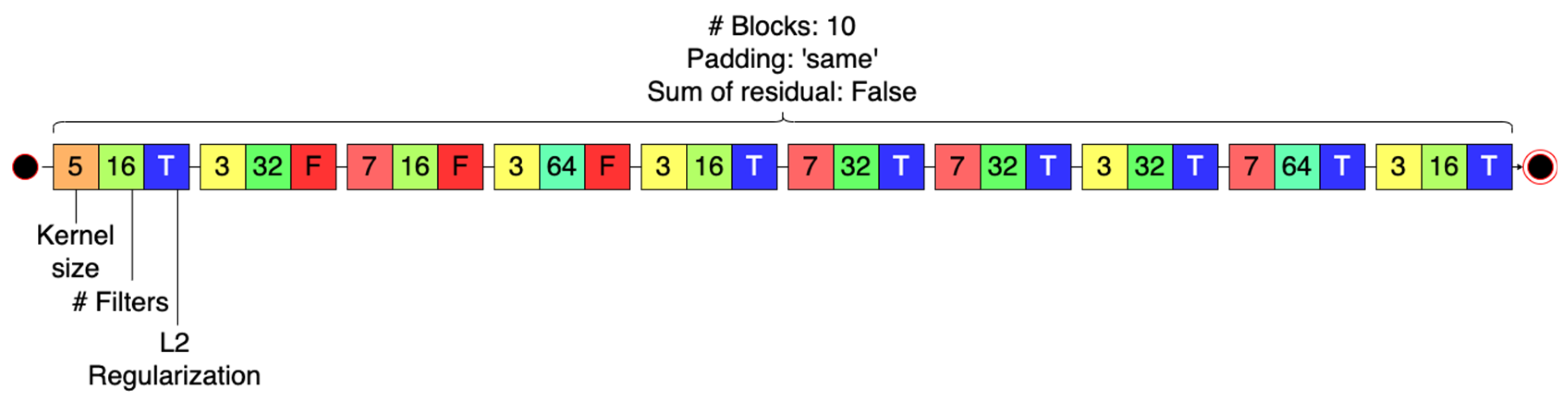
| Whole network | Number of blocks | 10 |
| Whole network | Sum of residuals before Activation layer | False |
| Convolutional blocks | Padding type | ‘same’ (for all blocks) |
| Convolutional blocks | Kernel size | 5, 3, 7, 3, 3, 7, 7, 3, 7, 3. |
| Convolutional blocks | Number of filters | 16, 32, 16, 64, 16, 32, 32, 32, 64, 16. |
| Convolutional blocks | L2 Regularization | True, False, False, False, True, True, True, True, True, True. |
| Scope | Variable | Values |
|---|---|---|
| Whole network | Number of blocks | 3 |
| Convolutional blocks | Padding type | ‘same’, ‘same’, ‘valid’. |
| Convolutional blocks | Kernel size | 3, 7, 3. |
| Convolutional blocks | Number of filters | 16, 16, 64. |
| Convolutional blocks | L2 Regularization | False, False, True. |
| Dataset | Search Space Topology | Surrogate Model | Optimal Found |
|---|---|---|---|
| CIFAR-10 | Type 1 | GP | 216.128 |
| CIFAR-10 | Type 1 | RF | 0.640 |
| CIFAR-10 | Type 2 | RF | 8196.919 |
| MNIST | Type 1 | GP | 2.537 |
| MNIST | Type 1 | RF | 3.778 |
| MNIST | Type 2 | RF | 1.468 |
Disclaimer/Publisher’s Note: The statements, opinions and data contained in all publications are solely those of the individual author(s) and contributor(s) and not of MDPI and/or the editor(s). MDPI and/or the editor(s) disclaim responsibility for any injury to people or property resulting from any ideas, methods, instructions or products referred to in the content. |
© 2024 by the authors. Licensee MDPI, Basel, Switzerland. This article is an open access article distributed under the terms and conditions of the Creative Commons Attribution (CC BY) license (https://creativecommons.org/licenses/by/4.0/).
Share and Cite
Pau, D.; Pisani, A.; Candelieri, A. Towards Full Forward On-Tiny-Device Learning: A Guided Search for a Randomly Initialized Neural Network. Algorithms 2024, 17, 22. https://doi.org/10.3390/a17010022
Pau D, Pisani A, Candelieri A. Towards Full Forward On-Tiny-Device Learning: A Guided Search for a Randomly Initialized Neural Network. Algorithms. 2024; 17(1):22. https://doi.org/10.3390/a17010022
Chicago/Turabian StylePau, Danilo, Andrea Pisani, and Antonio Candelieri. 2024. "Towards Full Forward On-Tiny-Device Learning: A Guided Search for a Randomly Initialized Neural Network" Algorithms 17, no. 1: 22. https://doi.org/10.3390/a17010022
APA StylePau, D., Pisani, A., & Candelieri, A. (2024). Towards Full Forward On-Tiny-Device Learning: A Guided Search for a Randomly Initialized Neural Network. Algorithms, 17(1), 22. https://doi.org/10.3390/a17010022