


An Adaptive Deep Learning Neural Network Model to Enhance Machine-Learning-Based Classifiers for Intrusion Detection in Smart Grids


Abstract
1. Introduction
2. Related Work
2.1. Classification Algorithms
2.2. Feature Extraction Methods
3. Proposed Adaptive Deep Learning
| Algorithm 1 Proposed ADL algorithm: where v is number of training data samples, is the key parameter to balance the training speed and classification accuracy, is the learning rate. N represents the set of neurons in the neural network; l is the number of neuron layers; D represents the dimension of the training data; and is the neuron. , , , and are the intermediate variables, denotes the weights, and is the bias. |
procedureADL() ▹ adaptive deep learning if is empty then end if if is empty then end if sizeof() while do end while while do use N to build the current layer and the neuron node end while output layer function for each training sample do calculate the actual output of the model end for return end procedure |
4. Results and Discussion
4.1. Preprocessing of Data
4.2. Performance Evaluation
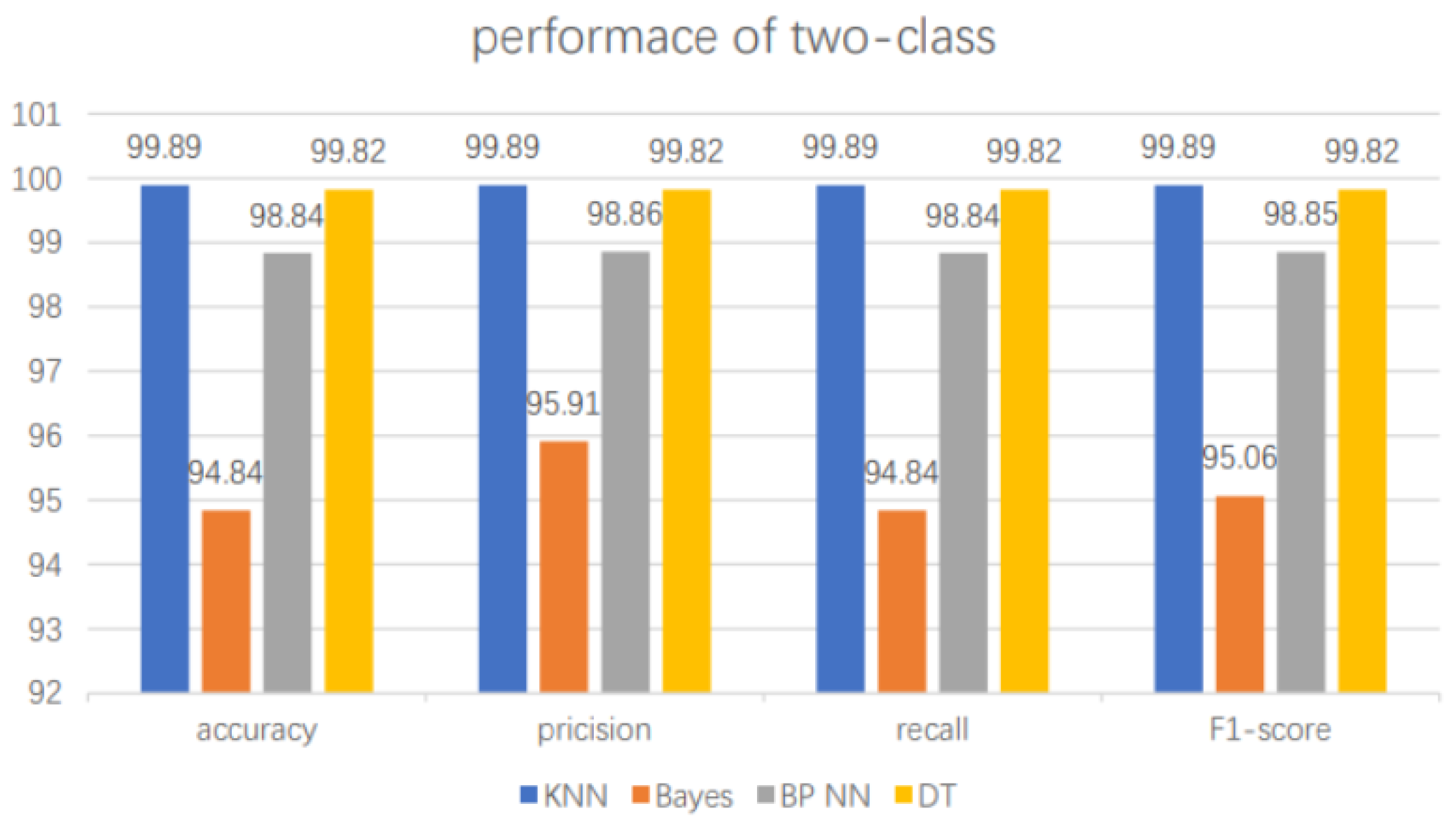
4.2.1. Two-Class Machine Learning Model
4.2.2. Multi-Class Machine Learning Model
5. Conclusions
Author Contributions
Funding
Data Availability Statement
Conflicts of Interest
References
- Zhang, Y.; Wang, L.; Xiang, Y. Power System Reliability Analysis With Intrusion Tolerance in SCADA Systems. IEEE Trans. Smart Grid 2016, 7, 669–683. [Google Scholar] [CrossRef]
- Nguyen, T.N.; Liu, B.-H.; Nguyen, N.P.; Chou, J.-T. Cyber Security of Smart Grid: Attacks and Defenses. In Proceedings of the ICC 2020—2020 IEEE International Conference on Communications (ICC), Dublin, Ireland, 7–11 June 2020. [Google Scholar]
- Harvey, M.; Long, D.; Reinhard, K. Visualizing NISTIR 7628, Guidelines for Smart Grid Cyber Security. In Proceedings of the 2014 Power and Energy Conference at Illinois (PECI), Champaign, IL, USA, 28 February–1 March 2014; pp. 1–8. [Google Scholar]
- Zhang, H.; Liu, B.; Wu, H. Smart Grid Cyber-Physical Attack and Defense: A Review. IEEE Access 2021, 9, 29641–29659. [Google Scholar] [CrossRef]
- Khan, S.; Kifayat, K.; Bashir, A.K.; Gurtov, A.; Hassan, M. Intelligent intrusion detection system in smart grid using computational intelligence and machine learning. Trans. Emerg. Telecommun. Technol. 2021, 32, e4062. [Google Scholar] [CrossRef]
- Meng, W.; Ma, R.; Chen, H.-H. Smart grid neighborhood area networks: A survey. IEEE Netw. 2014, 28, 24–32. [Google Scholar] [CrossRef]
- Khoei, T.T.; Slimane, H.O.; Kaabouch, N. A Comprehensive Survey on the Cyber-Security of Smart Grids: Cyber-Attacks, Detection, Countermeasure Techniques, and Future Directions. arXiv 2022, arXiv:2207.07738. [Google Scholar]
- Ding, J.; Qammar, A.; Zhang, Z.; Karim, A.; Ning, H. Cyber Threats to Smart Grids: Review, Taxonomy, Potential Solutions, and Future Directions. Energies 2022, 15, 6799. [Google Scholar] [CrossRef]
- Vaidya, B.; Makrakis, D.; Mouftah, H.T. Device authentication mechanism for Smart Energy Home Area Networks. In Proceedings of the 2011 IEEE International Conference on Consumer Electronics (ICCE), Las Vegas, NV, USA, 9–12 January 2011; pp. 787–788. [Google Scholar]
- Bae, H.-S.; Lee, H.-J.; Lee, S.-G. Voice recognition based on adaptive MFCC and deep learning. In Proceedings of the 2016 IEEE 11th Conference on Industrial Electronics and Applications (ICIEA), Hefei, China, 5–7 June 2016; pp. 1542–1546. [Google Scholar]
- Nicanfar, H.; Jokar, P.; Beznosov, K.; Leung, V.C.M. Efficient Authentication and Key Management Mechanisms for Smart Grid Communications. IEEE Syst. J. 2014, 8, 629–640. [Google Scholar] [CrossRef]
- Hao, J.; Kang, E.; Sun, J.; Wang, Z.; Meng, Z.; Li, X.; Ming, Z. An Adaptive Markov Strategy for Defending Smart Grid False Data Injection From Malicious Attackers. IEEE Trans. Smart Grid 2018, 9, 2398–2408. [Google Scholar] [CrossRef]
- Cui, J.; Long, J.; Min, E.; Mao, Y. WEDL-NIDS: Improving network intrusion detection using word embedding-based deep learning method. In MDAI 2018: Modeling Decisions for Artificial Intelligence; Springer: Berlin/Heidelberg, Germany, 2018; pp. 283–295. [Google Scholar]
- Song, C.; Sun, Y.; Han, G.; Rodrigues, J.J.P.C. Intrusion detection based on hybrid classifiers for smart grid. Comput. Electr. Eng. 2021, 93, 107212. [Google Scholar] [CrossRef]
- Hu, H.; Doufexi, A.; Armour, S.; Kaleshi, D. A Reliable Hybrid Wireless Network Architecture for Smart Grid Neighbourhood Area Networks. In Proceedings of the 2017 IEEE Wireless Communications and Networking Conference (WCNC), San Francisco, CA, USA, 19–22 March 2017; pp. 1–6. [Google Scholar]
- Gobena, Y.; Durai, A.; Birkner, M.; Pothamsetty, V.; Varakantam, V. Practical architecture considerations for Smart Grid WAN network. In Proceedings of the 2011 IEEE/PES Power Systems Conference and Exposition, Phoenix, AZ, USA, 20–23 March 2011; pp. 1–6. [Google Scholar]
- Mohi-ud-din, G. “NSL-KDD”, IEEE Dataport, Published by IEEE, USA. Available online: https://dx.doi.org/10.21227/425a-3e55 (accessed on 29 December 2018).
- Shone, N.; Ngoc, T.N.; Phai, V.D.; Shi, Q. A Deep Learning Approach to Network Intrusion Detection. IEEE Trans. Emerg. Top. Comput. Intell. 2018, 2, 41–50. [Google Scholar] [CrossRef]
- Dong, S.; Wang, P.; Abbas, K. A survey on deep learning and its applications. Comput. Sci. Rev. 2022, 40, 100379. [Google Scholar] [CrossRef]
- Jan, S.U.; Ahmed, S.; Shakhov, V.; Koo, I. Toward a Lightweight Intrusion Detection System for the Internet of Things. IEEE Access 2019, 7, 42450–42471. [Google Scholar] [CrossRef]
- Karimipour, H.; Dehghantanha, A.; Parizi, R.M.; Choo, K.-K.R.; Leung, H. A Deep and Scalable Unsupervised Machine Learning System for Cyber-Attack Detection in Large-Scale Smart Grids. IEEE Access. 2019, 7, 80778–80788. [Google Scholar] [CrossRef]
- Takiddin, A.; Ismail, M.; Zafar, U.; Serpedin, E. Deep Autoencoder-Based Anomaly Detection of Electricity Theft Cyberattacks in Smart Grids. IEEE Syst. J. 2022, 16, 4106–4117. [Google Scholar] [CrossRef]
- Inayat, U.; Zia, M.F.; Mahmood, S.; Berghout, T.; Benbouzid, M. Cybersecurity Enhancement of Smart Grid: Attacks, Methods, and Prospects. Electronics 2022, 11, 3854. [Google Scholar] [CrossRef]
- Zhou, F.; Wen, G.; Ma, Y.; Geng, H.; Huang, R.; Pei, L.; Yu, W.; Chu, L.; Qiu, R. A Comprehensive Survey for Deep-Learning-Based Abnormality Detection in Smart Grids with Multimodal Image Data. Appl. Sci. 2022, 12, 5336. [Google Scholar] [CrossRef]
- Berghout, T.; Benbouzid, M.; Muyeen, S.M. Machine learning for cybersecurity in smart grids: A comprehensive review-based study on methods, solutions, and prospects. Int. J. Crit. Infrastruct. Prot. 2022, 38, 100547. [Google Scholar] [CrossRef]
- Jithish, J.; Alangot, B.; Mahalingam, N.; Yeo, K.S. Distributed Anomaly Detection in Smart Grids: A Federated Learning-Based Approach. IEEE Access 2023, 11, 7157–7179. [Google Scholar] [CrossRef]
- Moustafa, N.; Slay, J. UNSW-NB15: A comprehensive data set for network intrusion detection systems (UNSW-NB15 network data set). In Proceedings of the 2015 Military Communications and Information Systems Conference (MilCIS), Canberra, Australia, 10–12 November 2015; pp. 1–6. [Google Scholar]


| Abbreviation | Term |
|---|---|
| ACE | asymmetric convolutional encoder |
| ADL | Adaptive deep learning |
| AMI | Advanced Metering Infrastructure |
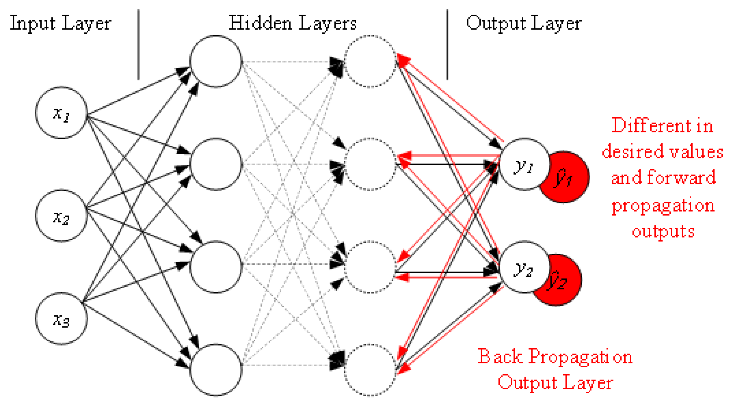
| BPNN | Back Propagation Neural Network |
| CFS | correlation-based feature selection |
| DBN | deep belief network |
| DDoS | distributed denial of service |
| DoS | denial-of-service |
| DT | Decision Tree |
| FDIA | false data injection attacks |
| HAN | Home Area Network |
| HEMS | home energy management system |
| IDS | Intrusion Detection System |
| IoT | Internet of Things |
| KDD | Knowledge Discovery in Databases |
| KNN | K-nearest neighbour |
| LSTM | long-short-term-memory |
| NISTIR | National Institute of Standards and Technology Interagency Report |
| NSL-KDD | Network Security Laboratory - Knowledge Discovery in Databases |
| R2L | root-to-local |
| ReLU | rectified linear activation function |
| SCADA | Supervisory Control And Data Acquisition |
| SDF | symbolic dynamic filtering |
| SVM | Support Vector Machine |
| U2R | user-to-root |
| WAN | Wide Area Network |
| Type | Attack | Description |
|---|---|---|
| Normal | Normal data traffic | Normal data type |
| DoS | Back, Land, Neptune, Pod, Smurf, Teardrop, Mailbomb, Processtable, UDPstorm, Apache2, Worm | Denial of service attacks, which make computers and networks unable to provide normal services |
| Probe | Satan, Nmap, Mscan, Saint, IP sweep, Portsweep | Port attack, scan port vulnerabilities to attack |
| U2R | Buffer overflow, Sql attack, XtermLoadmodule, Rootkit, Perl, Ps | Unauthorized users obtain root vulnerabilities through network vulnerabilities and perform illegal operations |
| R2L | Guess password, Imap, Multihop, Ftp write, Phf, Warezmaster, Xclock, Xsnoop, Snmpguess, Snmpgetattack, Sendmail, Httptunnel, Named | Remote attack, users remotely log in operate illegally through accounts and passwords |
| Works | Learning Type | Key Techniques | Datasets |
|---|---|---|---|
| [5] | Supervised | Particle swarm optimisation based neural network | KDD99 and NSL-KDD |
| [13] | Supervised | Work embedding-based deep learning | Intrusion Detection Evaluation Dataset (ISCX2012) |
| [14] | Semi-supervised | Long short-term memory and extreme gradient boosting with genetic algorithm | NSL-KDD |
| [18] | Unsupervised | Nonsymmetric deep autoencoder | KDD99 and NSL-KDD |
| [20] | Supervised | Support vector machine | Intrusion Detection Evaluation Dataset (CIC-IDS2017) |
| [21] | Unsupervised | Feature extraction using symbolic dynamic filtering | Data from testbed from Matpower |
| [22] | Supervised | Long short-term memory with stacked autoencoders | State Grid Corporation of China Dataset |
| [26] | Supervised | Federated Learning | KDD99, NSL-KDD and CIDDS-001 datasets |
| This work | Supervised | Adaptive deep learning using deep belief network | NSL-KDD |
| Model | (%) | (%) | (%) | (%) |
|---|---|---|---|---|
| kNN | 99.89 | 99.89 | 99.89 | 99.89 |
| kNN with ADL | 99.23 | 99.49 | 98.74 | 99.15 |
| Decision Tree | 99.82 | 99.82 | 99.82 | 99.82 |
| DT with ADL | 99.58 | 99.72 | 99.58 | 99.65 |
| Bayes | 94.84 | 95.91 | 94.84 | 95.06 |
| Bayes with ADL | 98.77 | 95.25 | 99.75 | 97.70 |
| BPNN | 98.84 | 98.86 | 98.84 | 98.05 |
| BPNN with ADL | 99.15 | 99.36 | 99.82 | 99.13 |
| Data Type | (%) | (%) | (%) | (%) |
|---|---|---|---|---|
| Normal | 99.24 | 98.86 | 99.43 | 99.81 |
| DoS | 99.85 | 99.86 | 98.85 | 99.85 |
| Probe | 95.64 | 97.42 | 95.43 | 96.41 |
| R2L | 84.13 | 91.23 | 83.23 | 87.07 |
| U2R | 28.49 | 66.88 | 28.57 | 40.02 |
| Data Type | (%) | (%) | (%) | (%) |
|---|---|---|---|---|
| Normal | 99.91 | 98.65 | 99.90 | 99.78 |
| DoS | 99.85 | 99.88 | 98.85 | 99.87 |
| Probe | 98.83 | 99.75 | 99.87 | 99.34 |
| R2L | 91.32 | 96.44 | 90.39 | 93.31 |
| U2R | 42.83 | 75.02 | 42.85 | 54.45 |
| Data Type | (%) | (%) | (%) | (%) |
|---|---|---|---|---|
| Normal | 99.58 | 100 | 97.2 | 83.9 |
| DoS | 99.76 | 97.5 | 99.3 | 89.7 |
| Probe | 99.81 | 84.7 | 99.7 | 91.6 |
| R2L | 24.36 | 55.6 | 99.7 | 90.3 |
| U2R | 60.17 | 82.3 | 99.7 | 72.08 |
| Data Type | (%) | (%) | (%) | (%) |
|---|---|---|---|---|
| Normal | 99.58 | 100 | 99.64 | 99.82 |
| DoS | 99.76 | 100 | 99.81 | 99.90 |
| Probe | 99.81 | 100 | 99.32 | 96.61 |
| R2L | 24.36 | 100 | 88.36 | 93.83 |
| U2R | 10.17 | 41.32 | 47.23 | 44.08 |
Disclaimer/Publisher’s Note: The statements, opinions and data contained in all publications are solely those of the individual author(s) and contributor(s) and not of MDPI and/or the editor(s). MDPI and/or the editor(s) disclaim responsibility for any injury to people or property resulting from any ideas, methods, instructions or products referred to in the content. |
© 2023 by the authors. Licensee MDPI, Basel, Switzerland. This article is an open access article distributed under the terms and conditions of the Creative Commons Attribution (CC BY) license (https://creativecommons.org/licenses/by/4.0/).
Share and Cite
Li, X.J.; Ma, M.; Sun, Y. An Adaptive Deep Learning Neural Network Model to Enhance Machine-Learning-Based Classifiers for Intrusion Detection in Smart Grids. Algorithms 2023, 16, 288. https://doi.org/10.3390/a16060288
Li XJ, Ma M, Sun Y. An Adaptive Deep Learning Neural Network Model to Enhance Machine-Learning-Based Classifiers for Intrusion Detection in Smart Grids. Algorithms. 2023; 16(6):288. https://doi.org/10.3390/a16060288
Chicago/Turabian StyleLi, Xue Jun, Maode Ma, and Yihan Sun. 2023. "An Adaptive Deep Learning Neural Network Model to Enhance Machine-Learning-Based Classifiers for Intrusion Detection in Smart Grids" Algorithms 16, no. 6: 288. https://doi.org/10.3390/a16060288
APA StyleLi, X. J., Ma, M., & Sun, Y. (2023). An Adaptive Deep Learning Neural Network Model to Enhance Machine-Learning-Based Classifiers for Intrusion Detection in Smart Grids. Algorithms, 16(6), 288. https://doi.org/10.3390/a16060288