Analysis and Prediction of Wear Performance of Different Topography Surface


Abstract
1. Introduction
2. Numerical Simulation of Sliding Wear Process
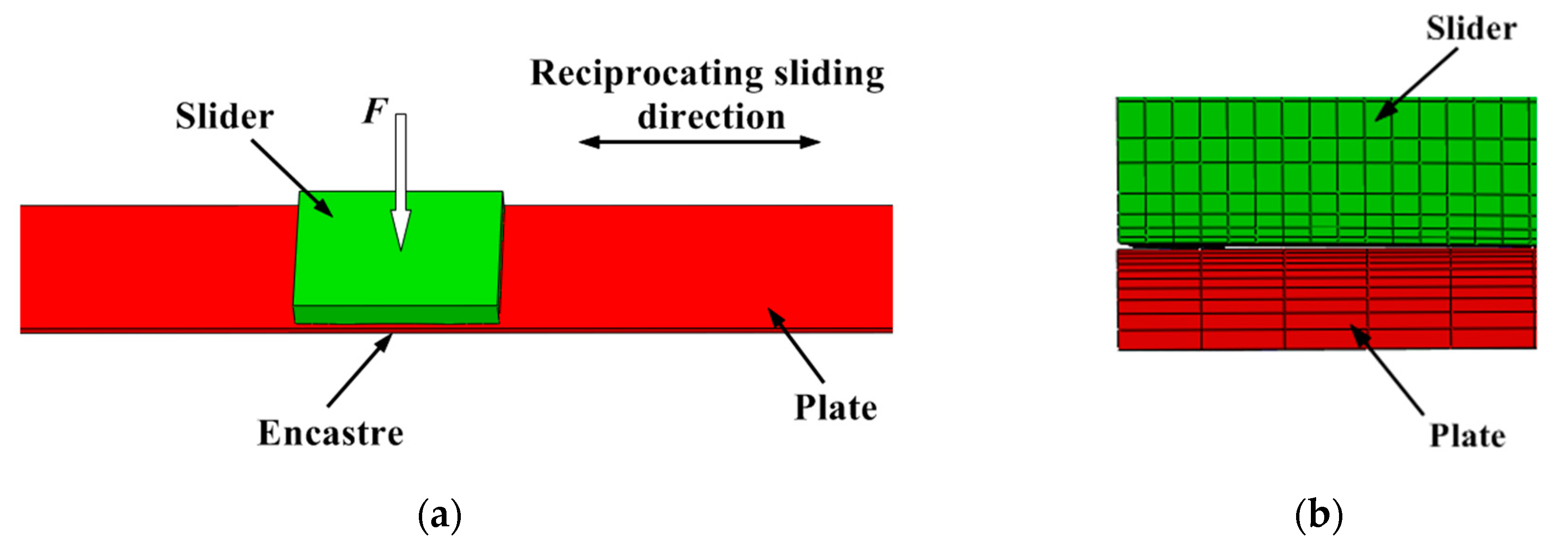
2.1. Wear Simulation Model
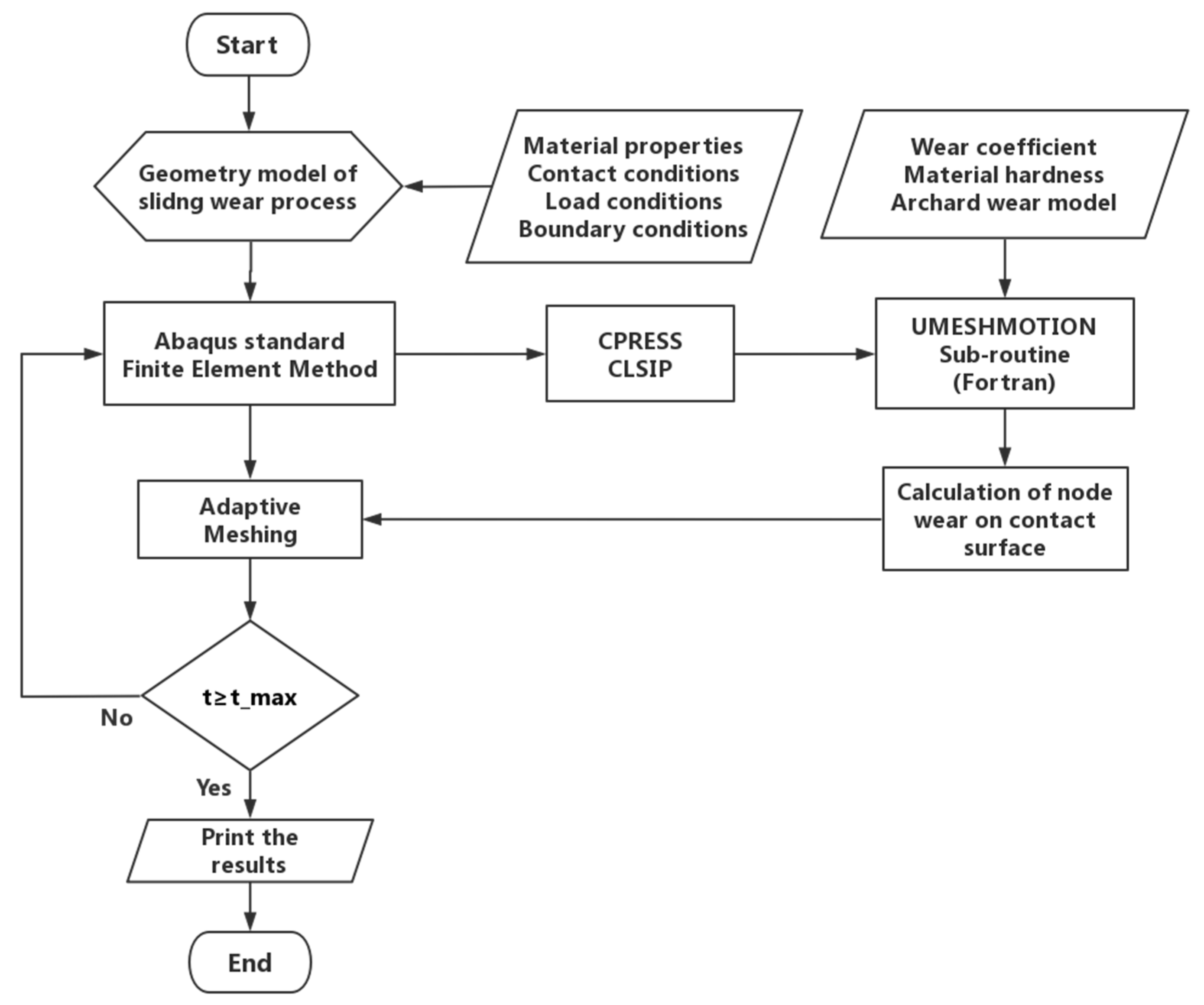
2.2. Wear Simulation Procedure
2.3. Numerical Simulation Method of Wear
3. Grey System Theory
3.1. Grey Incidence Operator
3.2. Grey Incidence Analysis
3.3. Grey Prediction Model
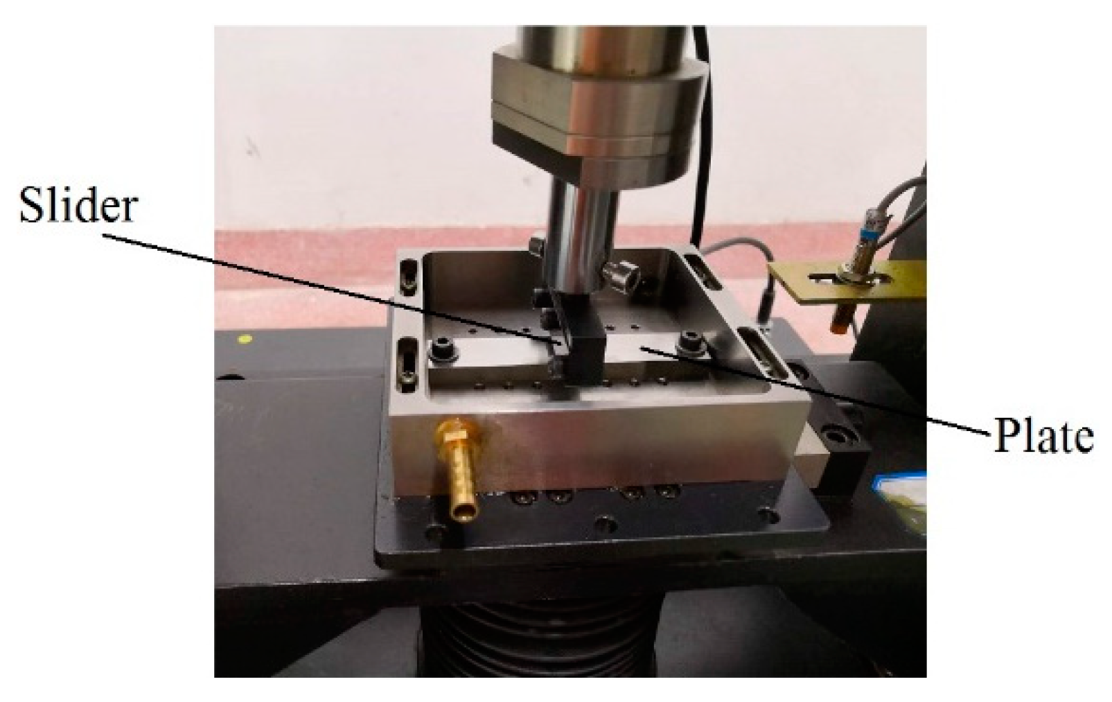
4. Experimental Procedure
5. Results and Discussion
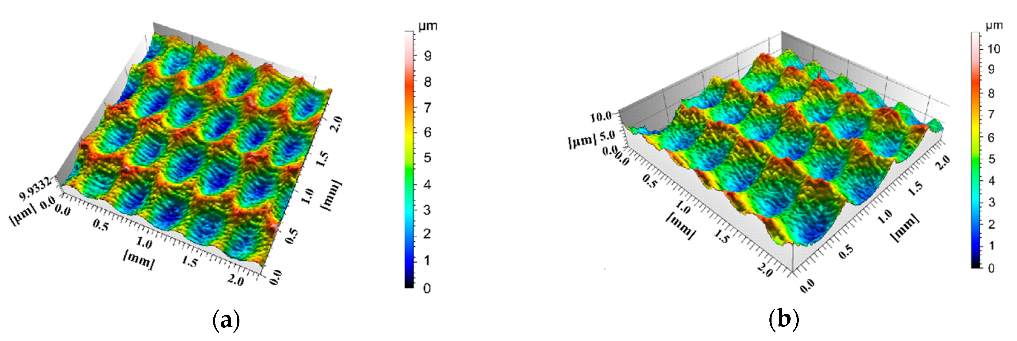
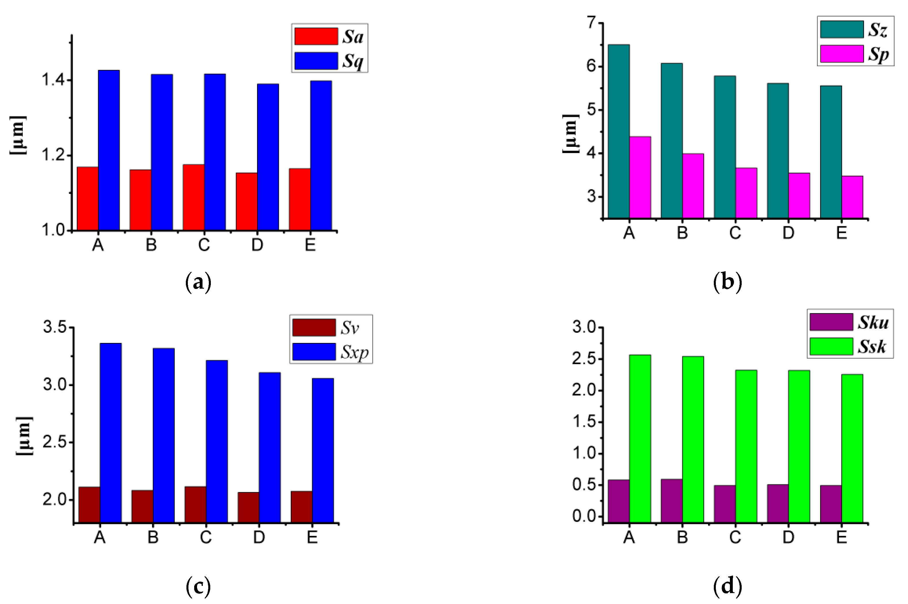
5.1. Surface Texture Roughness Parameters
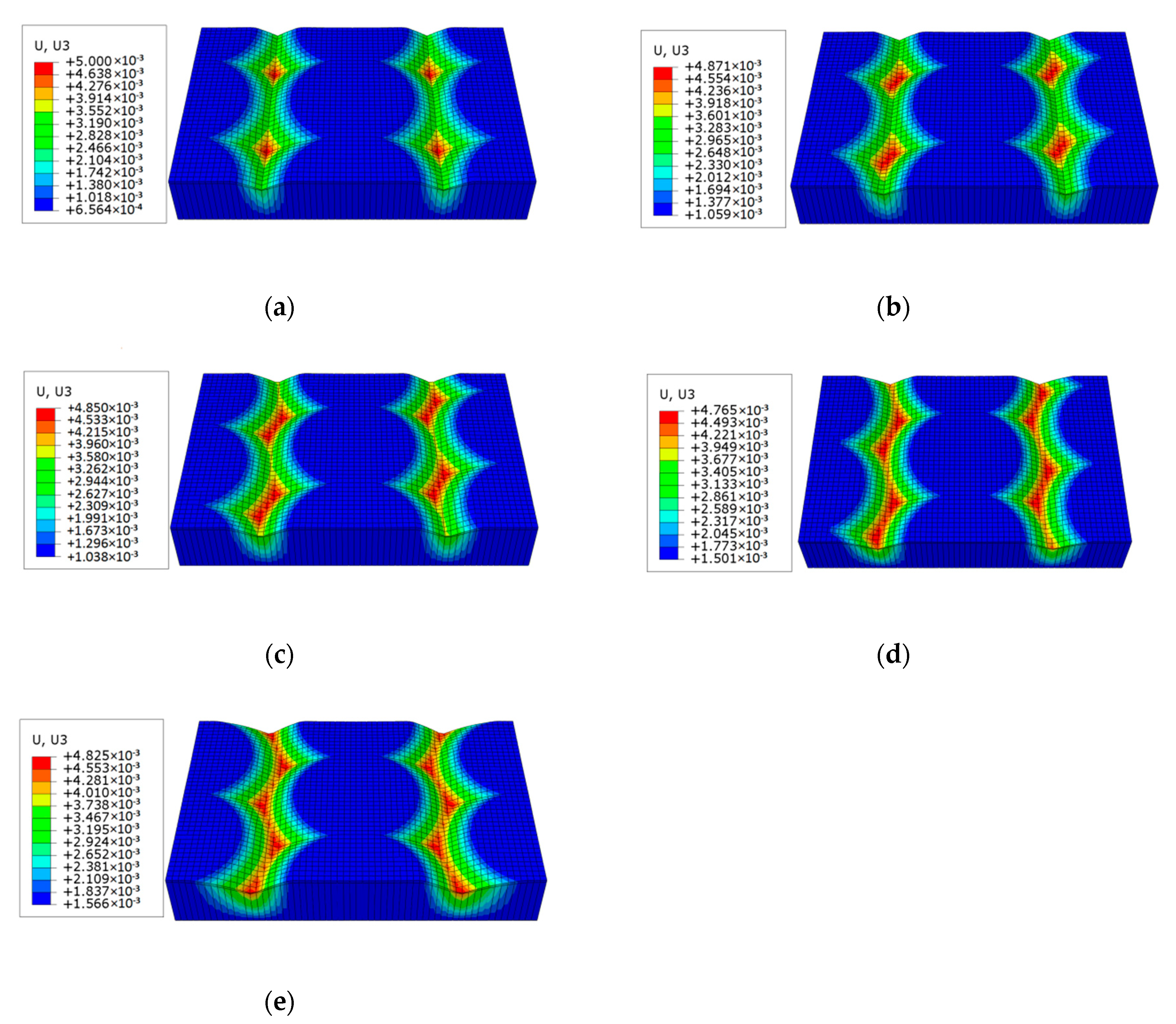
5.2. Wear Simulation Analysis
5.3. Grey Incidence Analysis
5.4. Grey Prediction Model
6. Experimental Results
7. Conclusions
- (1)
- Under dry friction conditions, the wear resistance was not directly related to the topography offset distance and the shape of the surface topography, but it was closely related to the surface texture roughness parameters.
- (2)
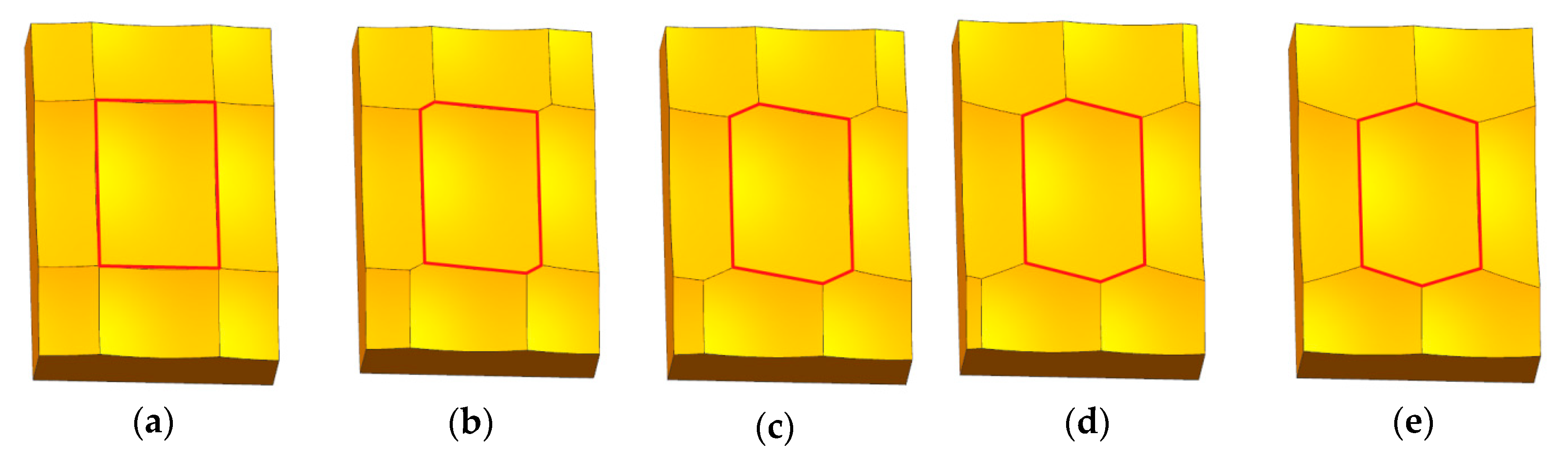
- With the increase of the offset distance, the surface topography shape gradually changes from a quadrilateral pit to an axisymmetric hexagonal pit. The value of Sz, Sp, Sxp, and Sku gradually becomes smaller, while the value of Sa, Sq, Sv, and Ssk shows an oscillating changes characteristics.
- (3)
- Quantitative analysis of the relevance between the surfaces wear resistance and the surface texture roughness parameters under dry friction conditions, and found that there was a strong relevance between Sa, Sv, Sq, Sxp, Sku, and Ssk and the wear resistance, that is, the surface wear resistance can be accurately characterized by the six surface texture roughness parameters.
- (4)
- A zeroth order six variables grey model, GM(0,6), was established for prediction the wear characteristic parameter ΔVs, which provided a new idea for the prediction and judgment of the wear resistance of different surface topography.
Author Contributions
Funding
Conflicts of Interest
Nomenclature
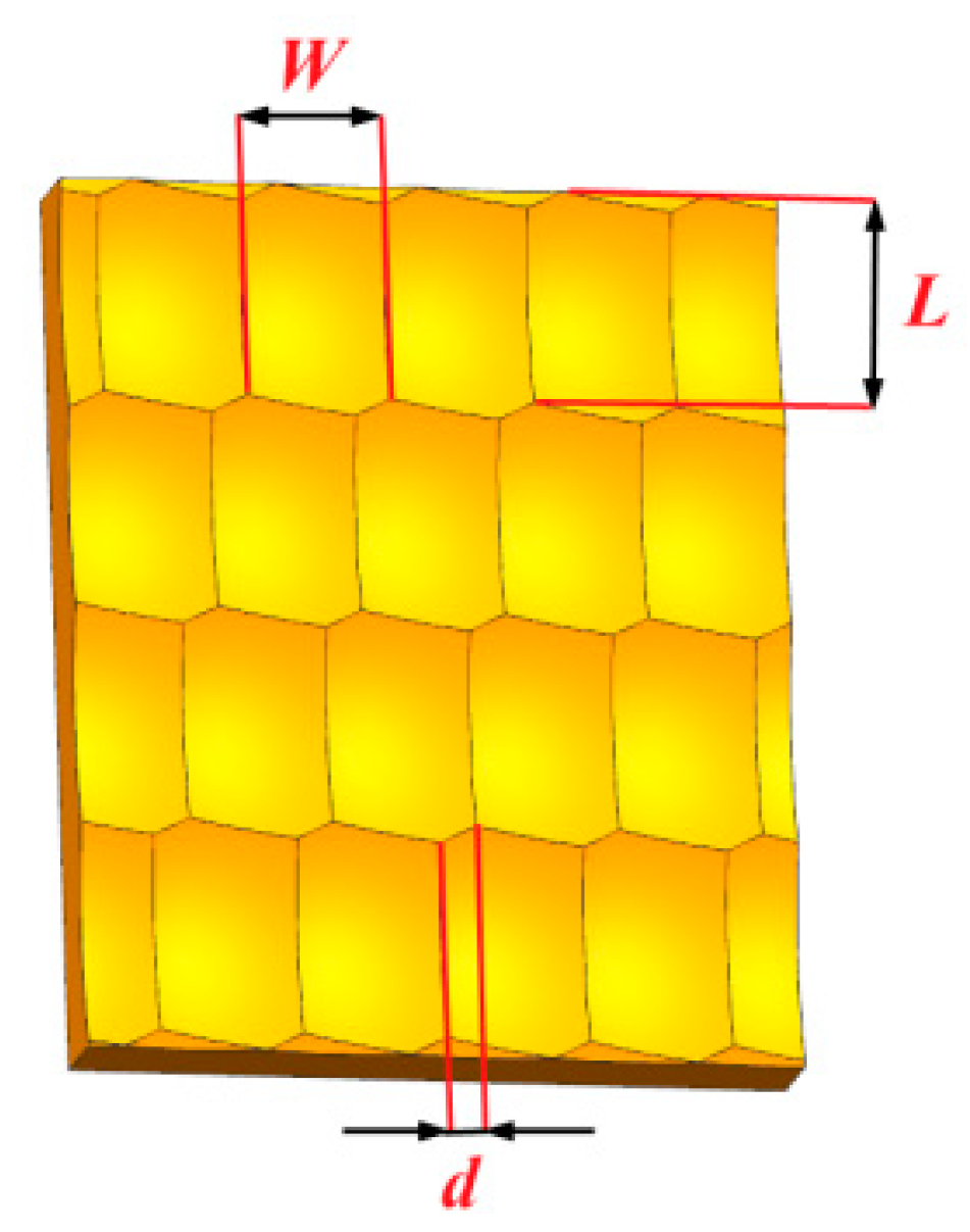
| W | Pit width |
| L | Pit length |
| d | Topography offset distance |
| hs | Slider height |
| hp | Pit height |
| Sa | Arithmetical mean height |
| Sq | Root mean square height |
| Sz | Largest height |
| Sp | Largest peak height |
| Sv | Largest pit height |
| Ssk | Skewness |
| Sku | Kurtosis |
| Sxp | Difference in height between the 2.5% and 50% material ratio |
References
- Laukkanen, A.; Holmberg, K.; Ronkainen, H.; Waudby, R.; Stachowaiak, G.; Wolski, M.; Podsiadlo, P.; Gee, M.; Nunn, J.; Gachot, C.; et al. Topographical orientation effects on friction and wear in sliding DLC and steel contacts, part 1: Experimental. Wear 2015, 330, 3–22. [Google Scholar] [CrossRef]
- Xing, Y.; Deng, J.; Feng, X.; Yu, S. Effect of laser surface texturing on Si3N4/TiC ceramic sliding against steel under dry friction. Mater. Des. 2013, 52, 234–245. [Google Scholar] [CrossRef]
- Zhang, H.; Dong, G.N.; Hua, M. Improvement of Tribological Behaviors by Optimizing Concave Texture Shape Under Reciprocating Sliding Motion. J. Tribol. 2017, 139, 011701. [Google Scholar] [CrossRef]
- Dzierwa, A. Influence of Steel Surface Preparation Method on Topography and Tribological Behaviour in Dry Sliding Conditions. Key Eng. Mater. 2016, 674, 265–270. [Google Scholar] [CrossRef]
- Etsion, I. State of the art in laser surface texturing. J. Tribol. 2005, 127, 248–253. [Google Scholar] [CrossRef]
- Yu, H.; Wang, X.; Zhou, F. Geometric Shape Effects of Surface Texture on the Generation of Hydrodynamic Pressure between Conformal Contacting Surfaces. Tribol. Lett. 2010, 37, 123–130. [Google Scholar] [CrossRef]
- Yu, H.; Deng, H.; Huang, W.; Wang, X. The effect of dimple shapes on friction of parallel surfaces. Proc. Inst. Mech. Eng. Part J J. Eng. Tribol. 2011, 225, 693–703. [Google Scholar] [CrossRef]
- Nuraliza, N.; Syahrullail, S.; Razak, D.; Azwadi, C. Influence of Micro-Pits on Sliding Motion Under Low Speeds for Block-On-Disk Tribotester. Part. Sci. Technol. 2015, 34, 754–763. [Google Scholar] [CrossRef]
- Wang, B.; Chang, Q.; Qi, Y. Effect of laser surface texture on the tribological properties of different materials under dry friction. Mocaxue Xuebao Tribol. 2014, 34, 408–413. [Google Scholar]
- Tang, W.; Zhou, Y.; Zhu, H.; Yang, H. The effect of surface texturing on reducing the friction and wear of steel under lubricated sliding contact. Appl. Surf. Sci. 2013, 273, 199–204. [Google Scholar] [CrossRef]
- Sedlăcek, M.; Podgornik, B.; Vižintin, J. Influence of surface preparation on roughness parameters, friction and wear. Wear 2008, 266, 482–487. [Google Scholar] [CrossRef]
- Sedlăcek, M.; Podgornik, B.; Vižintin, J. Correlation between standard roughness parameters skewness and kurtosis and tribological behaviour of contact surfaces. Tribol. Int. 2012, 48, 102–112. [Google Scholar] [CrossRef]
- Zhang, H.; Liu, Y.; Hua, M. An optimization research on the coverage of micro-textures arranged on bearing sliders. Tribol. Int. 2018, 128, 231–239. [Google Scholar] [CrossRef]
- Zhu, S.; Huang, P. Influence mechanism of morphological parameters on tribological behaviors based on bearing ratio curve. Tribol. Int. 2017, 109, 10–18. [Google Scholar] [CrossRef]
- Ghosh, A.; Sadeghi, F. A novel approach to model effects of surface roughness parameters on wear. Wear 2015, 338, 73–94. [Google Scholar] [CrossRef]
- Andrzej, D.; Angeolos, M. Influence of Ball-Burnishing Process on Surface Topography Parameters and Tribological Properties of Hardened Steel. Machines 2019, 7, 11. [Google Scholar] [CrossRef]
- Tang, L.; Yin, J.; Sun, Y.; Shen, H.; Gao, C. Chip formation mechanism in dry hard high-speed orthogonal turning of hardened AISI D2 tool steel with different hardness levels. Int. J. Adv. Manuf. Technol. 2017, 93, 2341–2356. [Google Scholar] [CrossRef]
- Zheng, M.; Wang, B.; Zhang, W.; Cui, Y.; Zhang, L.; Zhao, S. Analysis and prediction of surface wear resistance of ball-end milling topography. Surf. Topogr. Metrol. Prop. 2020, 8, 025032. [Google Scholar] [CrossRef]
- Zhao, X.; Zhang, P.; Wen, Z. On the coupling of the vertical, lateral and longitudinal wheel-rail interactions at high frequencies and the resulting irregular wear. Wear 2019, 430, 317–326. [Google Scholar] [CrossRef]
- Arunachalam, A.; Idapalapati, S. Material removal analysis for compliant polishing toll using adaptive meshing technique and Archard wear model. Wear 2019, 418, 140–150. [Google Scholar] [CrossRef]
- Albers, A.; Reichert, S. On the influence of surface roughness on the wear behavior in the running-in phase in mixed-lubricated contacts with the finite element method. Wear 2017, 376, 1185–1193. [Google Scholar] [CrossRef]
- Chen, H.; Jin, L.; Li, X. Grey Systems: Theory and Application. Grey Syst. Theory Appl. 2011, 4883, 44–45. [Google Scholar] [CrossRef]
- Liu, S.; Yang, Y.; Forrest, J. Grey Data Analysis. Comput. Risk Manag. 2017, 10, 978–981. [Google Scholar] [CrossRef]
- The International Organization for Standardization (ISO). PN-EN 25178-2:2012 Geometrical Product Specifications (GPS)—Surface Texture: Areal—Part 2: Terms, Definitions and Surface Texture Parameters; ISO: Geneva, Switzerland, 2012. [Google Scholar]


| Groups | A | B | C | D | E |
|---|---|---|---|---|---|
| Topography offset distance (d/mm) | 0 | 0.05 | 0.1 | 0.15 | 0.2 |
| Slider height (hs/mm) | 0.206502 | 0.206075 | 0.205783 | 0.205613 | 0.205557 |
| Pit height (hp/μm) | 6.5021 | 6.0750 | 5.7829 | 5.6129 | 5.5571 |
| Material | Elastic Modulus (GPa) | Poisson’s Ratio | Density (kg/m3) |
|---|---|---|---|
| Cr12MoV | 218 | 0.28 | 7700 |
| Groups | Length (L/mm) | Width (W/mm) | Pit Height (hp/μm) | Topography Offset Distance (d/mm) |
|---|---|---|---|---|
| F | 0.6 | 0.4 | 9.9332 | 0.17 |
| G | 0.6 | 0.4 | 10.7779 | 0.08 |
| Groups | Sa (μm) | Sq (μm) | SZ (μm) | Sp (μm) | Sv (μm) | Ssk | Sku | Sxp (μm) |
|---|---|---|---|---|---|---|---|---|
| F | 1.4275 | 1.7222 | 9.9332 | 5.4729 | 4.4603 | 0.0361 | 2.2774 | 3.1434 |
| G | 1.3283 | 1.6267 | 10.7779 | 11.4509 | 4.7049 | 0.2559 | 2.4257 | 2.6645 |
| Groups | Sz (μm) | Sp (μm) | Sv (μm) | Sq (μm) | Sa (μm) | Sku | Ssk | Sxp (μm) |
|---|---|---|---|---|---|---|---|---|
| A | 6.5021 | 4.3890 | 2.1131 | 1.4267 | 1.1693 | 2.5658 | 0.5831 | 3.3631 |
| B | 6.0750 | 3.9916 | 2.0834 | 1.4152 | 1.1619 | 2.5428 | 0.5953 | 3.3185 |
| C | 5.7829 | 3.6669 | 2.1160 | 1.4164 | 1.1755 | 2.3241 | 0.4927 | 3.2143 |
| D | 5.6129 | 3.5459 | 2.0670 | 1.3897 | 1.1534 | 2.3205 | 0.5074 | 3.1079 |
| E | 5.5571 | 3.4810 | 2.0761 | 1.3984 | 1.1648 | 2.2578 | 0.4952 | 3.0575 |
| Groups | A | B | C | D | E |
|---|---|---|---|---|---|
| V (×10−3/mm3) | 0.589303 | 0.589569 | 0.588276 | 0.584946 | 0.583111 |
| ∆Vs (×10−3/μm2) | 0.7857 | 0.7861 | 0.7844 | 0.7799 | 0.7775 |
| Groups | ΔVs | Sz | Sp | Sv | Sq | Sa | Sku | Ssk | Sxp |
|---|---|---|---|---|---|---|---|---|---|
| A | 1 | 1 | 1 | 1 | 1 | 1 | 1 | 1 | 1 |
| B | 1.0005 | 0.9343 | 0.9095 | 0.9859 | 0.9919 | 0.9937 | 0.9910 | 1.0209 | 0.9867 |
| C | 0.9983 | 0.8894 | 0.8355 | 1.0014 | 0.9928 | 1.0053 | 0.9058 | 0.8450 | 0.9558 |
| D | 0.9926 | 0.8632 | 0.8079 | 0.9782 | 0.9741 | 0.9864 | 0.9044 | 0.8702 | 0.9241 |
| E | 0.9895 | 0.8547 | 0.7931 | 0.9825 | 0.9802 | 0.9962 | 0.8800 | 0.8493 | 0.9091 |
| Parameters | SZ | Sp | Sv | Sq | Sa | Sku | Ssk | Sxp |
|---|---|---|---|---|---|---|---|---|
| γ | 0.7901 | 0.7446 | 0.9729 | 0.9662 | 0.9974 | 0.8386 | 0.8061 | 0.8785 |
| Groups | Real Data (μm2) | Simulated Value (ΔVs(1)) (μm2) | Simulated Value (ΔVs(0)) (μm2) | Errors (μm2) | Relative Errors (%) |
|---|---|---|---|---|---|
| A | 0.7857 | 0.7857 | 0.7857 | 0 | 0 |
| B | 0.7861 | 1.5716 | 0.7859 | −0.0002 | 0.0254 |
| C | 0.7844 | 2.3558 | 0.7840 | −0.0004 | 0.0510 |
| D | 0.7799 | 3.1356 | 0.7794 | −0.0005 | 0.0641 |
| E | 0.7775 | 3.9130 | 0.7769 | −0.0006 | 0.0772 |
| Groups | m0 (g) | m1 (g) | T (s) | s (mm) | ΔVs (μm2) |
|---|---|---|---|---|---|
| F | 62.5750 | 62.5492 | 598 | 89700 | 37.3540 |
| G | 62.4101 | 62.3825 | 598 | 89700 | 39.9600 |
Publisher’s Note: MDPI stays neutral with regard to jurisdictional claims in published maps and institutional affiliations. |
© 2020 by the authors. Licensee MDPI, Basel, Switzerland. This article is an open access article distributed under the terms and conditions of the Creative Commons Attribution (CC BY) license (http://creativecommons.org/licenses/by/4.0/).
Share and Cite
Wang, B.; Zheng, M.; Zhang, W. Analysis and Prediction of Wear Performance of Different Topography Surface. Materials 2020, 13, 5056. https://doi.org/10.3390/ma13225056
Wang B, Zheng M, Zhang W. Analysis and Prediction of Wear Performance of Different Topography Surface. Materials. 2020; 13(22):5056. https://doi.org/10.3390/ma13225056
Chicago/Turabian StyleWang, Ben, Minli Zheng, and Wei Zhang. 2020. "Analysis and Prediction of Wear Performance of Different Topography Surface" Materials 13, no. 22: 5056. https://doi.org/10.3390/ma13225056
APA StyleWang, B., Zheng, M., & Zhang, W. (2020). Analysis and Prediction of Wear Performance of Different Topography Surface. Materials, 13(22), 5056. https://doi.org/10.3390/ma13225056