Abstract
This paper describes and presents an experimental program of low-cycle fatigue tests of austenitic stainless steel 08Ch18N10T at room temperature. The low-cycle tests include uniaxial and torsional tests for various specimen geometries and for a vast range of strain amplitude. The experimental data was used to validate the proposed cyclic plasticity model for predicting the strain-range dependent behavior of austenitic steels. The proposed model uses a virtual back-stress variable corresponding to a cyclically stable material under strain control. This internal variable is defined by means of a memory surface introduced in the stress space. The linear isotropic hardening rule is also superposed. A modification is presented that enables the cyclic hardening response of 08Ch18N10T to be simulated correctly under torsional loading conditions. A comparison is made between the real experimental results and the numerical simulation results, demonstrating the robustness of the proposed cyclic plasticity model.
1. Introduction
Austenitic stainless steels, for example, 316L in PWR (pressurized water reactor) and 08Ch18N10T in the Russian VVER concept (water–water power reactor), are usually used for components in primary circuit reactor internals (a block consisting of guided tubes, a core barrel, a core barrel bottom and a core shroud), in main primary pipes, and so forth. During their design life, these components must withstand mechanical operational loads (e.g., pressure pulses and vibrations), thermal loads (regimes such as heating up and shut-downs), corrosive loads and also irradiation. These regimes subject the reactor internals to cyclic loading.
When designing or assessing the long term operation of existing structural components, it is necessary to include fatigue evaluations. In the last decade, the finite element method (FEM) with phenomenological models has mainly been used in practical applications [1]. A description and a short history of the development of constitutive models of cyclic plasticity has been provided by the authors in a previous publication [2]. Their goal is to describe as accurately as possible the stress-strain behavior of the material, which is found on the basis of experiments under cyclic loading conditions [3]. A small deviation in the stress-strain prediction can lead to a major fatigue error, especially in low cycle fatigue. In this case, stainless steels show cyclic hardening in the initial stage, followed by cyclic softening [4,5]. This phenomenon depends on the strain range and also on the type of loading. Non-proportional loading induces more cyclic hardening than proportional loadings. The most sensitive materials are materials with low stacking fault energy, for example, austenitic stainless steels [6]. Low-cycle fatigue tests of this type were presented for example, by Jin et al. in Reference [7]. They presented results for 316L stainless steel under proportional and non-proportional loadings. In another study, Xing et al. [8] presented the results of experimental testing on 316L stainless steel under proportional and non-proportional loadings with various strain amplitudes. The authors also presented a numerical study and compared the numerical results with the experimental data. They used the visco-plastic numerical model, based on the Ohno-Wang kinematic hardening rule.
The temperature in VVER concept reactor usually does not exceed 350 in most components. Temperature effect have significant influence, which is presented in Reference [9]. The additional hardening due to non-proportional loading has been investigated by many authors. The basic concept involves modifying the isotropic or kinematic hardening rule with a non-proportional parameter. For example, Benallal and Marquis [10] introduced the non-proportional angle, which is defined as the angle between the direction of the increment in plastic deformation and the direction of the deviatoric stress. Another approach was introduced by Tanaka [11]. He introduced the fourth rank tensor, which characterizes the internal dislocation structure of the material. This parameter is dependent on the loading path.
The goal of all the studies mentioned above was to understand the behavior of the material under specific cyclic loading conditions and to provide the material data for a better fatigue and lifetime assessment of the structural parts. This paper follows up on the main author’s previous paper [2] which presents some results of uniaxial low-cycle fatigue tests of austenitic stainless steel 08Ch18N10T at room temperature. The experimental program includes uniaxial tests of hourglass-type specimens and is now extended by new results for notched specimens with 3 different notch geometries considering strain amplitudes up to 3%. Torsional loading tests of notched-tube specimens are also newly presented.
In a previous paper [2], the authors presented a new constitutive material model that is used for finite element (FE) simulations of experiments on 08Ch18N10T material. The constitutive material model is based on the Chaboche model. The proposed material model is in very good agreement with uniaxial loading condition results. In this paper, the model has been modified to provide a better description of the torsional loading. This modification also enables the cyclic hardening response of 08Ch18N10T steel to be simulated correctly under torsional loading conditions. The constitutive material model is based on the memory surface introduced in the stress space, which is analogous to the theory of Jiang and Sehitoglu [12] for treating the impact of the strain amplitude on the stress response of the material. The new theory is shown on the kinematic hardening rule based on Chaboche’s model with three backstress parts. Recently, an approach has been introduced that takes into account a new internal variable called virtual backstress, corresponding to a cyclically stable material. This provides an easy way to identify the parameters and to reduce the number of material parameters. A comparison between the real experimental results and the numerical simulation results demonstrates the robustness of the constitutive plasticity model.
2. Experiments
The experimental section describes the low-cycle fatigue test measurements of specimens in pure tension/compression mode and in torsion mode.
2.1. Experimental Setup
Pure axial tension-compression tests were carried out using a MAYES electromechanical testing machine with a loading capacity of . The test specimens were placed in MTS 646 hydraulic collet grips to ensure repeatability of the alignment conditions in tensile/compression mode. The axial deformation of the specimens was controlled by an MTS 634.25 extensometer with an initial gage length of 10 mm with a 50% measuring range, for uniform gage specimens and with an initial length of 20 mm with a 20% measuring range, for elliptically-shaped specimens.
Pure torsion tests were conducted on an MTS Bionix servo-hydraulic testing machine with an axial load capacity of and in torsion. The test specimens were carefully mounted in MTS 647 hydraulic wedge grips and were tested with the axial load control set to zero. An EPSILON 3550 axial/torsional extensometer was employed to measure and control the torsional shear angle with a range of . The initial gauge length of the extensometer was . The whole test setup is shown in Figure 1.
Figure 1.
Experiment: (a) Experimental Setup, (b) digital image correlation (DIC) Snapshot of Specimen IDF-6.
These tests were conducted at room temperature and were loaded using a triangular waveform at a strain rate of . During the experimental measurements all channels were recorded, for example, time, force/torque, displacement/angle, axial/torsional extensometer, with a recording frequency of .
The digital image correlation (DIC) was used for an analysis of the 3D deformation on the surface of some specimens, see Figure 1. During cyclic loading, the frame rate was set to cover at least per one loading cycle. The MERCURY RT optical measuring system was used to capture and analyze the 3D images. The configuration of the system consists of two CMOS BONITO cameras with circular polarizing filters to reduce the glare from the reflected surface of the specimen.
The test setup (see Figure 1) on the MTS servo-hydraulic testing machine consists of hydraulic wedge grips, a notched specimen and an EPSILON axial/torsional extensometer and a snapshot of a notched specimen (see Figure 1) under a loading with a random contrast pattern, which the DIC algorithm requires and a strain map on the surface.
The stochastic pattern on the surface of the specimen and two digital video cameras allows 3D strain measurements throughout the fatigue life until fracture, with resolution of 1100 DPI (1 px = 0.22 μm). In addition, the DIC system can continuously store all captured images in the computer memory. The fatigue life of each loading condition takes at least several dozen of cycles, even tens of thousands of cycles, which can generate up to hundreds of thousands of images to be processed. All captured images were processed later in post processing to prevent data loss. This loss occurs when the bitrate increases while real-time processing is being used.
2.2. Experimental Program
The experimental program consists of 6 series of specimens. The first series is used for the material parameter identification process. According to the ASTM E606 standard [13], the classic uniform-gage geometry of a specimen is limited to a total strain amplitude of = 0.5%. For higher strain levels, non-uniform hour-glass type geometry is required in order to prevent buckling. The material parameters identification series (IDF) was therefore compiled from uniform-gage (UG) specimens (see Figure 2) and non-uniform-gage specimens with an elliptical longitudinal section (E9, see Figure 2). To identify the material parameters (described in detail in Reference [2]), it is necessary to know the stress-strain curves in the cycles. For UG specimen geometry, tested according to Reference [13], this can be calculated directly from the elongation of the extensometer and from the force measured during the experiment. For E9 specimen geometry, the strain was measured by the DIC (due to the experimental setup, the strain cannot be calculated directly from the elongation of the extensometer for non-uniform gage geometries).
Figure 2.
IDF Specimen Geometry: (a) UG, (b) E9.
The next series consists of E9 geometry (see Figure 2), notch geometry with an (R1.2, see Figure 3), geometry with an notch (R2.5, see Figure 3) and geometry with an notch (R5, see Figure 4). The last series is the notched tube geometry (NT, see Figure 4), which was exposed to torsional loading.
Figure 3.
Notched Specimens: (a) R1.5, (b) R2.5.
Figure 4.
Notched and Notched Tube Specimens: (a) R5, (b) NT.
All boundary conditions of the experiments and their simulations are together with resulting experimental lifetimes reported in Appendix A.
3. Constitutive Model with Strain Range Dependency
The concept of single yield surface plasticity with strain range dependency is used. Isothermal conditions are considered, since the influence of the strain rate is not taken into account. The constitutive model is described in detail in Reference [2], so just a brief recapitulation of some key equations is presented here.
3.1. Cyclic Plasticity and Memory Surface
The plasticity function is defined as
where is the deviatoric part of stress tensor , is the deviatoric part of back-stress . The actual yield surface size Y is defined as
where R is the isotropic variable and is the initial size of the yield surface. The accumulated plastic strain increment is defined as
The superposition of the virtual back stress parts is defined as
and for each part
For 08Ch18N10T material, three backstress parts are taken into consideration, so .
The evolution of the memory surface size is directed by the following rule
where
and
3.2. Isotropic Hardening
The cyclic isotropic hardening is linear in p, defined incrementally as
where
where , , and are material parameters.
3.3. Kinematic Hardening
Chaboche’s kinematic hardening rule is used in this study. The backstress is composed of M parts
the memory term is a function of memory surface and accumulated plastic strain p
where M, and are the same as in Equation (5). Function is defined as
where is a material parameter. is a function defined as follows
where , , , , , , , and are material parameters.
3.4. Modification for Torsional Loading
The original plasticity model shows very good prediction under uniaxial loading conditions [2]. The original model also predicts well for notched specimen geometries but produces an error of up to about 15% under shear stress loading conditions, as will be shown in Section 6. For a low loading level (see Figure 5a)), where there is limited cyclic hardening, the prediction of the original model [2] is satisfactory. For a high loading level (see Figure 5b)), the model overpredicts the cyclic hardening under dominant shear stress loading conditions and the formulation of the material model needs to be modified.
Figure 5.
Original model under torsional loading: (a) specimen NT-1 (low loading level), (b) specimen NT-6 (high loading level).
The first modification of the original model [2] is to separate the memory surface function into two memory surfaces. Memory surface for the isotropic hardening part remains the same as in the original model defined by the set of Equations (4)–(8). The new memory surface for the kinematic hardening part is modified and is defined by analogy as
where
where is Kronecker delta, I, J are indexes of stress tensor and is a new material parameter. The rest of the equations for defining the memory surface of the kinematic hardening part remain analogous to the original model [2]:
where
and
A quick analysis of this modified formulation shows that it provides practically the same prediction in uniaxial loading conditions (because ) as the original formulation. However, depending on the value of , it can give a different prediction under shear loading conditions: it is more effective for higher loading levels than for lower loading levels and it can reduce the over prediction of the model for .
The second modification to the original model [2], also associated with the memory surface, is to omit limits and and to set boundaries of the memory surfaces instead: and . The value of the memory surface and used for controlling the isotropic and kinematic hardening part can lie only between these two bounds. For simplification and for mathematically correct expression, the memory surface size that is used, , is defined as
and analogously for . The variable in Equations (13)–(18) of the original model is simply replaced by variable . The modified form of the kinematic hardening equations is now
The third modification of the original model [2] is the definition of the formulation of isotropic hardening as a non-linear formulation in p as
where , and are material parameters. This very important modification deserve a short analysis. In the original model [2], for cyclic loading, the actual yield stress Y increases practically linearly with the number of cycles. This means that with many cycles, the actual yield stress Y can theoretically go higher than the total stress amplitude and the computed deformation becomes only elastic.
4. Identification of Material Parameters
The material parameter identification process for 08Ch18N10T is based on knowing the shape of the stress-strain hysteresis loops during the fatigue life. A total of twelve uniaxial specimens and eight torsional specimens are used for the identification process. This is described in detail in References [14] and [2], so just a brief recapitulation of the key steps updated by the unique features of the proposed modification to the material model is done here.
The Young modulus E, the Poisson ratio and the yield strength are obtained from a tensile test. The actual yield strength evolution during the fatigue life is determined using the root mean square error method. Chaboche material parameters , , , , , are identified from two selected hysteresis loops (the bigger loop and the smaller loop).
The first guess of the memory surface size for each specimen is computed. It is assumed here that . Boundary parameters and are simply the maximum and minimum values of computed in the identification process.
The actual yield stress is fitted as a function of and parameters , , are found from Equation (33).
Using the experimental data from the tensile test and performing a simulation of this test, parameter is found based on the Equation (13) as an optimal value of . The value of function from Equation (13) is found, using a similar optimization process as for determining the Chaboche material parameters. is the value of for , where is the number of cycles after which the crack occurs on the specimen and the force starts to drop during the experiment. From Equation (16), is then set as a function of by finding material parameters , , , , .
For each NT geometry specimen tested, the value in each cycle between the experimental amplitude of torque and the simulation amplitude of torque can be defined as
The over all cycles is calculated as
where index n is the number of cycles. The total error over all NT geometry specimens tested is defined as
where s is the NT specimen index and is the total number of NT specimens tested (see Table A3 in Appendix A for details).
For the different from Equation (21), the value is captured in Figure 6. The final material parameter is identified as the optimal value of where the is minimal.
Figure 6.
Identification of material parameter .
The material value parameters are presented in Table 1.
Table 1.
Material parameters of the new proposed model for 08Ch18N10T.
The experimental data from the IDF series of experiments can also be plotted into fatigue diagram -, where is the number of cycles to failure and is the amplitude of the total strain. Due to the experimental setup, is not completely constant during the experiment in the case of E9 geometry (during the experiments, the amplitude of extensometer elongation is controlled to be constant, so for UG geometry the is also constant but it is not completely constant for E9 geometry), so the mean value during the experiment is plotted. Fatigue data are shown in Figure 7. Other lifetimes are reported in the form of tabular data in Appendix A.
Figure 7.
Fatigue data of the IDF series of experiments.
5. FE Simulations
The geometry of most specimens is not uniform, so the non-uniform stress and strain field in their cross-section are expected and FEA must be used for simulations. The constitutive model is implemented into Abaqus FE software using the USDFLD subroutine. FE models of each of the tested geometries were created, see Figure 8, Figure 9 and Figure 10. The symmetry boundary condition is defined on the right edge of the model. The left edge of the model always corresponds with the cross-section where the extensometer is attached to the body of the specimen during the experiment. The displacement boundary condition on the upper edge of the FE model is created with the same amplitude value as was recorded from the extensometer during the experiment. Abaqus CAX8R mesh elements are used for the axisymmetric models and C3D8R elements are used for the NT geometry, which is a 3D model with cyclic symmetry. The element size in fine mesh areas has been determined using sensitivity study to .
Figure 8.
FE model: (a) UG, (b) E9.
Figure 9.
FE model: (a) R1.2, (b) R2.5.
Figure 10.
FE model: (a) R5, (b) NT.
The Abaqus Chaboche plasticity material model with combined hardening and the USDFLD subroutine is used. The equations of the constitutive model are coded into the USDFLD subroutine for calculating the actual memory surfaces size and , which, combined with the accumulated plastic strain p, determines the actual yield stress Y, the value of function and the memory term of the Chaboche model . The full Abaqus USDFLD subroutine code written in Fortran is available in Appendix B.
This subroutine makes possible to use the material model presented here in engineering computations. Combined with the material parameters identification process described in Section 4, it can also be used for other materials.
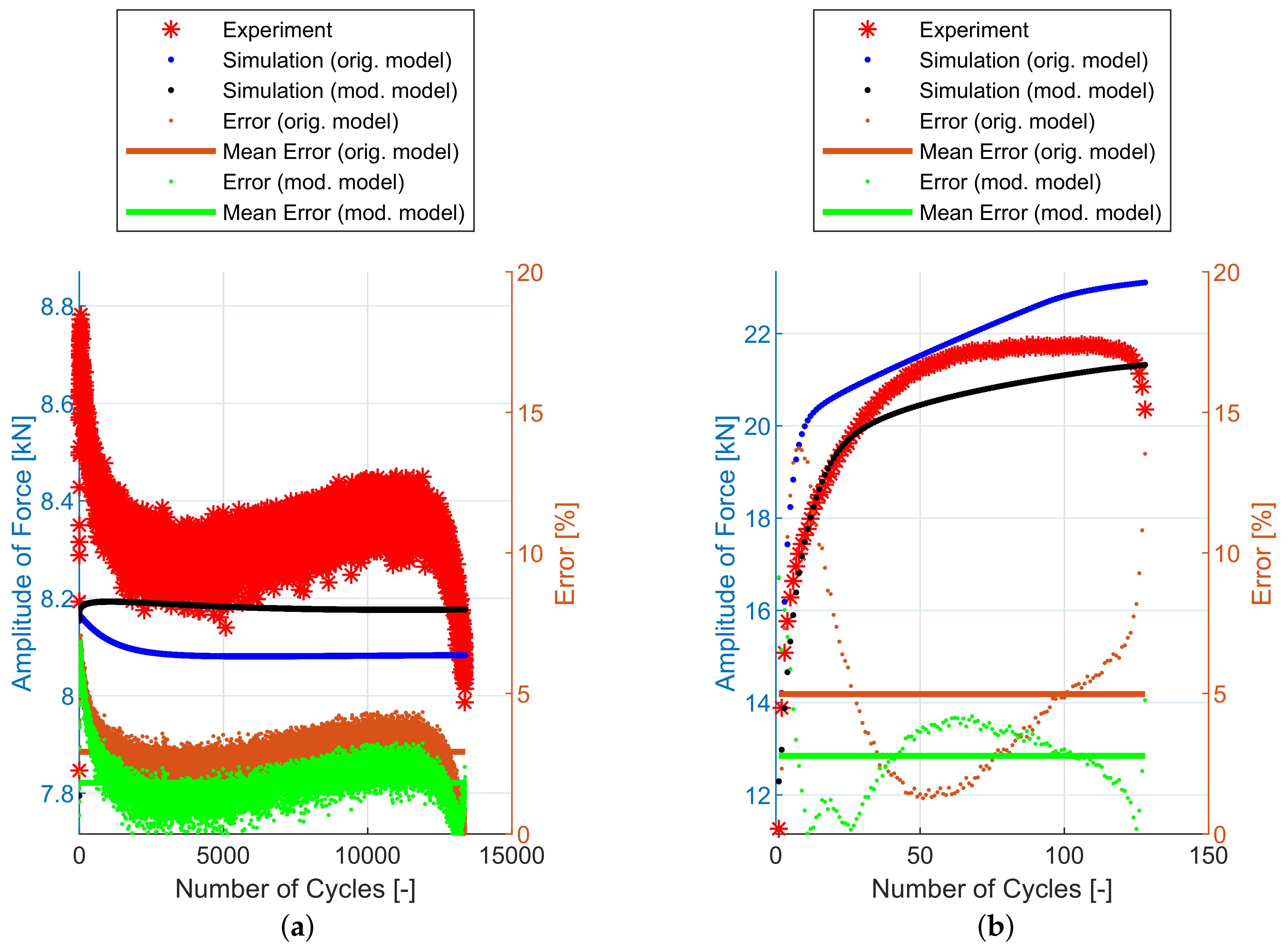
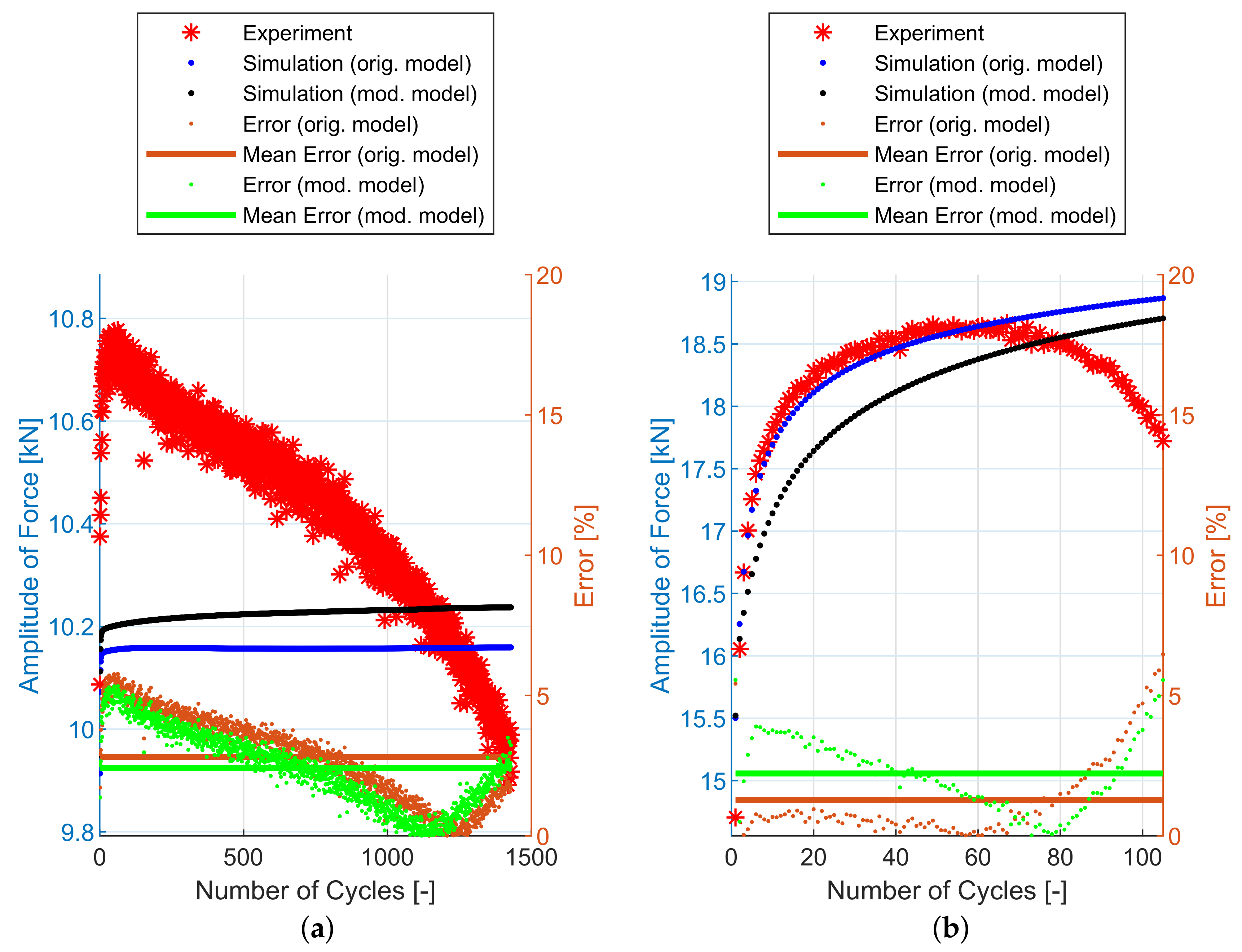
6. Experimental and Simulation Results
The implementation of the plasticity model presented here (including the presented modification) into FE code was verified using FE simulations of all experiments mentioned in Section 2.2. The following figures show some results of experiments and their FE simulations. Due to the large scale of the experimental program, only two representative specimens with low and high load levels were selected for demonstration in this section. The results of remaining specimens are presented in the form of error values in following tables. The compared variables in each figure are the amplitudes of the force measured during the experiment () and computed by the FE simulations (). Two constitutive models are shown—the original model [2] and the modified model presented in this paper. The actual error between each FE simulation and the experiment and the mean error value, are also displayed.
The error between the experiment and the FE simulation in each cycle n is calculated simply as
The mean error and the total error are calculated using Equations (35) and (36) considering corresponding number of specimens in the series.
The Figure 11 and Table 2 show the experimental and simulation results of E9 geometry series representing the uniaxial loading conditions. The prediction capability of these two models is comparable.
Figure 11.
Amplitude of force—experiment vs. simulations [2]: (a) E9-1, (b) E9-17.
Table 2.
Mean error of all E9 specimens tested—experiment vs. simulations [2].
The NT geometry series results are in Figure 12 and Table 3. In this case, the compared variables are the amplitudes of the torque measured during the experiment () and computed by the FE simulations (). The errors are calculated using Equations (34)–(36). For this geometry, the difference in the prediction capability of the original model and the modified model is not the same—the modified model provides a better prediction of the cyclic hardening of the material under torsional loading for high loading levels.
Figure 12.
Amplitude of force—experiment vs. simulations: (a) NT-1, (b) NT-6.
Table 3.
Mean error of all NT specimens tested—experiment vs. simulations.
Finally, the notched specimen geometry series R1.2, R2.5 and R5 follows on Figure 13, Figure 14 and Figure 15 and Table 4, Table 5 and Table 6. The stress field in the cross-section of these specimens is no longer uniaxial and the prediction capabilities of both models are also comparable.
Figure 13.
Amplitude of force—experiment vs. simulations: (a) R1.2-1, (b) R1.2-18.
Figure 14.
Amplitude of force—experiment vs. simulations: (a) R2.5-1, (b) R2.5-21.
Figure 15.
Amplitude of force—experiment vs. simulations: (a) R5-1, (b) R5-24.
Table 4.
Mean error of all R1.2 specimens tested—experiment vs. simulations.
Table 5.
Mean error of all R2.5 specimens tested—experiment vs. simulations.
Table 6.
Mean error of all R5 specimens tested—experiment vs. simulations.
7. Discussion
As has been shown in the previous sections, the model proposed in Reference [2] can capture very well the static and cyclic stress-strain curve for uniaxial loading conditions with a reasonable number of material parameters. Using the modification proposed in this paper, with only two extra material parameters, the error under torsional loading conditions can be reduced significantly, without any harm under uniaxial loading conditions, as is shown in Table 7, where the total errors (defined in Equation (36)) are summarized. Both models also produce very good predictions for notched specimen geometries, where the stress-strain field is not uniaxial.
Table 7.
Total error comparison between the original model and the modified model.
In Figure 11, Figure 12, Figure 13, Figure 14 and Figure 15, the range of response quantity axis has been chosen to make visible the difference between experimental values and predicted ones. That is why the error seems to be higher than actually is. This is true especially in case of the lowest strain amplitude.
In the calibration process dealing with torsional loading, the value is found as a compromise between all loading levels, so the proposed modification improves prediction for most, but not all, specimens tested (see Table 3 and Table 7).
It should be pointed out that presented tests consist only of single loading modes. Combinations of these modes, for example, proportional and also non-proportional combination of tension and torsion probably induces cyclic non-proportional hardening and another cyclic phenomenons. These conditions are also limiting for eventual FE analysis on the real components. Combined loading conditions considering proportional as well as non-proportional loading are potential topics for future investigation.
8. Conclusions
This paper has described the experimental setup and the experimental program for a low-cycle fatigue test of 08Ch18N10T austenitic stainless steel. Using FE simulations, material model [2] capable of capturing the strain-range dependent cyclic hardening has been newly verified on notched specimens, where the stress-strain field is non-uniform and for torsional loading. With a newly proposed modification, model can correctly simulate cyclic hardening also for shear stress loading conditions.
The extensive experimental program was subsequently completely simulated. The Chaboche plasticity model combined with non-linear isotropic hardening has already been implemented into Abaqus commercial FE software. The model presented here can easily be implemented into Abaqus using the USDFLD subroutine as a simple extension of the Abaqus default cyclic plasticity model. The full Fortran code of subroutine can be found in Appendix B. This implementation makes the proposed model ready to use for some engineering computations. The usage limitations are given by the conditions under which the model has been tested (simple, uncombined loading).
The original cyclic plasticity model presented in [2] provides a good prediction of the cyclic response of uniaxial and notched specimens. With the modification for torsional loading that has been presented here, it can also provide a good prediction of cyclic hardening under torsional loading conditions. It can also easily be applied to the Abdel-Karim-Ohno model or to a modified version with promised ratcheting prediction [8]. The model can be extended by standard techniques for use in the area of viscoplasticity [15].
The calibration of the cyclic plasticity model was described briefly in this paper and was used with experimental data available for 08Ch18N10T. In future work, an automated process for identifying material parameters could be prepared in a similar way as in [16]. Some authors of this paper also work on the material parameters identification using results from DIC measurements in order to reduce number of necessary specimens for recently expensive technologies of 3D printing of metals [17].
Author Contributions
Conceptualization, J.F., R.H. and M.Š.; Data curation, R.P.; Investigation, J.F., R.P. and M.Š.; Methodology, J.F. and R.H.; Software, J.F.; Supervision, R.H. and M.Š.; Validation, J.F.; Visualization, J.F. and R.P.; Writing—original draft, J.F., R.H. and P.G.; Writing—review & editing, J.F., R.H., P.G. and M.Š.
Funding
This research was funded by the Czech Science Foundation (GACR), grant No. 19-03282S (Influence of Complex and Cyclic Loading Modes on Lifetime of Machine Parts Made by Additive Manufacturing) and by The Technology Agency of the Czech Republic in the frame of the project TN01000024 National Competence Center-Cybernetics and Artificial Intelligence. The paper has been done in connection with project Innovative and additive manufacturing technology—new technological solutions for 3D printing of metals and composite materials, reg. no. CZ.02.1.01/0.0/17_049/0008407 financed by Structural Founds of Europe Union.
Conflicts of Interest
The authors declare no conflict of interest.
Abbreviations
The following abbreviations are used in this manuscript:
| DIC | digital image correlation |
| IDF | identification specimen series |
| FE | finite element |
| FEM | finite element method |
| UG | uniform-gage |
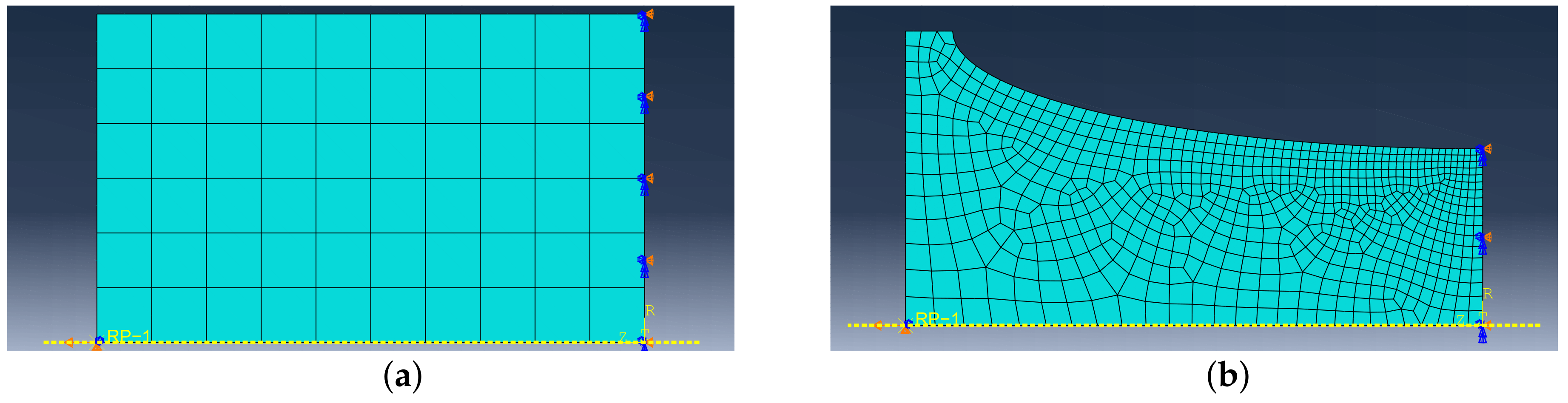
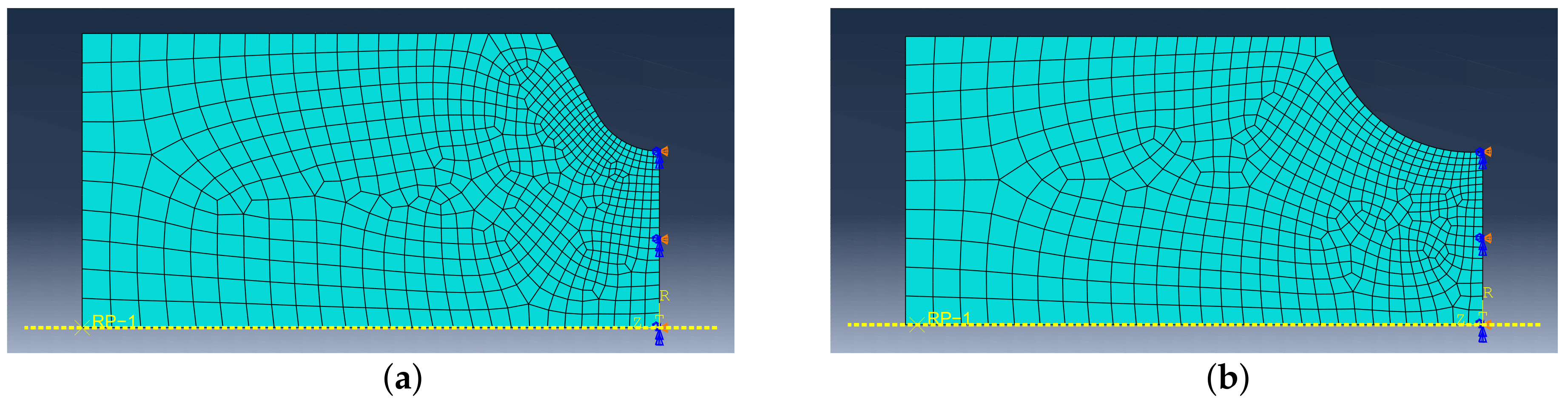
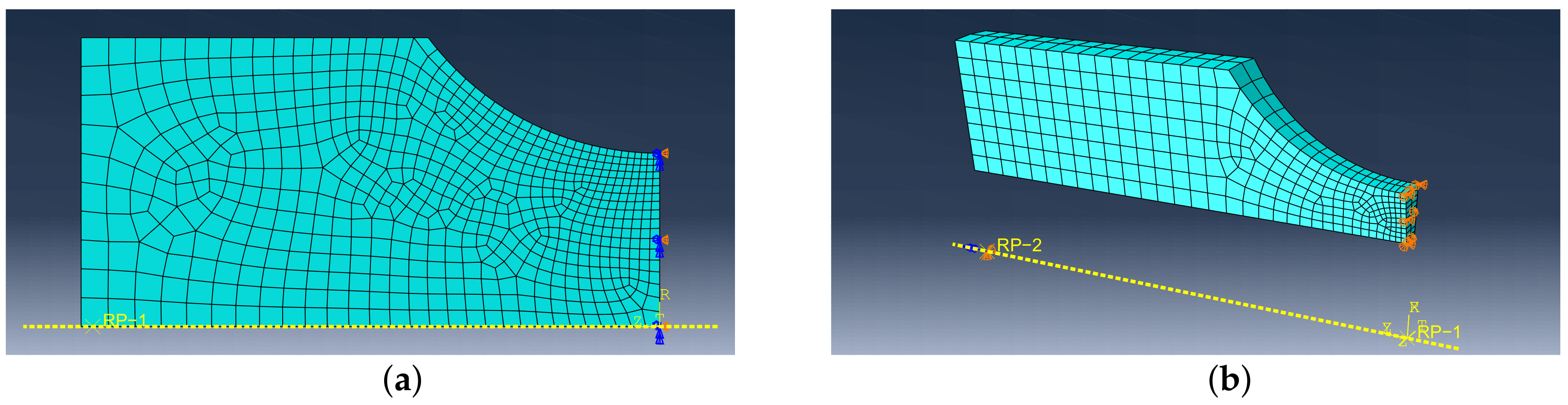
Appendix A. Boundary Conditions of Simulations
Table A1.
Boundary conditions of IDF specimens.
Table A1.
Boundary conditions of IDF specimens.
| Specimen Name | Geometry Type | ||
|---|---|---|---|
| IDF-1 | UG | 0.030 | 37509 |
| IDF-2 | UG | 0.050 | 4285 |
| IDF-3 | UG | 0.075 | 916 |
| IDF-4 | UG | 0.100 | 580 |
| IDF-5 | UG | 0.125 | 254 |
| IDF-6 | E9 | 0.132 | 159 |
| IDF-7 | E9 | 0.154 | 381 |
| IDF-8 | E9 | 0.176 | 370 |
| IDF-9 | E9 | 0.198 | 161 |
| IDF-10 | E9 | 0.245 | 156 |
| IDF-11 | E9 | 0.264 | 124 |
| IDF-12 | E9 | 0.353 | 93 |
Table A2.
Boundary conditions of E9 specimens.
Table A2.
Boundary conditions of E9 specimens.
| Specimen Name | Geometry Type | ||
|---|---|---|---|
| E9-1 | E9 | 0.0447 | 13382 |
| E9-2 | E9 | 0.0446 | 15104 |
| E9-3 | E9 | 0.0662 | 4053 |
| E9-4 | E9 | 0.0662 | 3887 |
| E9-5 | E9 | 0.0881 | 1529 |
| E9-6 | E9 | 0.0880 | 1853 |
| E9-7 | E9 | 0.1100 | 1158 |
| E9-8 | E9 | 0.1100 | 631 |
| E9-9 | E9 | 0.1320 | 748 |
| E9-10 | E9 | 0.1540 | 546 |
| E9-11 | E9 | 0.1770 | 406 |
| E9-12 | E9 | 0.1980 | 332 |
| E9-13 | E9 | 0.2200 | 253 |
| E9-14 | E9 | 0.2420 | 181 |
| E9-15 | E9 | 0.2420 | 195 |
| E9-16 | E9 | 0.2640 | 220 |
| E9-17 | E9 | 0.3520 | 128 |
Table A3.
Boundary conditions of NT specimens.
Table A3.
Boundary conditions of NT specimens.
| Specimen Name | Geometry Type | ||
|---|---|---|---|
| NT-1 | NT | 0.8703 | 5006 |
| NT-2 | NT | 0.8694 | 6894 |
| NT-3 | NT | 1.1423 | 2222 |
| NT-4 | NT | 1.1414 | 2289 |
| NT-5 | NT | 1.4031 | 2045 |
| NT-6 | NT | 1.3772 | 1532 |
| NT-7 | NT | 1.6554 | 1170 |
| NT-8 | NT | 2.1492 | 925 |
Table A4.
Boundary conditions of R1.2 specimens.
Table A4.
Boundary conditions of R1.2 specimens.
| Specimen Name | Geometry Type | ||
|---|---|---|---|
| R1.2-1 | R1.2 | 0.0245 | 1429 |
| R1.2-2 | R1.2 | 0.0246 | 946 |
| R1.2-3 | R1.2 | 0.0326 | 715 |
| R1.2-4 | R1.2 | 0.0406 | 523 |
| R1.2-5 | R1.2 | 0.0407 | 490 |
| R1.2-6 | R1.2 | 0.0489 | 290 |
| R1.2-7 | R1.2 | 0.0485 | 356 |
| R1.2-8 | R1.2 | 0.0560 | 241 |
| R1.2-9 | R1.2 | 0.0563 | 256 |
| R1.2-10 | R1.2 | 0.0639 | 134 |
| R1.2-11 | R1.2 | 0.0642 | 202 |
| R1.2-12 | R1.2 | 0.0721 | 171 |
| R1.2-13 | R1.2 | 0.0718 | 164 |
| R1.2-14 | R1.2 | 0.0794 | 112 |
| R1.2-15 | R1.2 | 0.0868 | 145 |
| R1.2-16 | R1.2 | 0.0869 | 114 |
| R1.2-17 | R1.2 | 0.0945 | 96 |
| R1.2-18 | R1.2 | 0.0944 | 105 |
Table A5.
Boundary conditions of R2.5 specimens.
Table A5.
Boundary conditions of R2.5 specimens.
| Specimen Name | Geometry Type | ||
|---|---|---|---|
| R2.5-1 | R2.5 | 0.0228 | 5875 |
| R2.5-2 | R2.5 | 0.0341 | 1245 |
| R2.5-3 | R2.5 | 0.0340 | 1041 |
| R2.5-4 | R2.5 | 0.0454 | 607 |
| R2.5-5 | R2.5 | 0.0454 | 761 |
| R2.5-6 | R2.5 | 0.0568 | 378 |
| R2.5-7 | R2.5 | 0.0567 | 429 |
| R2.5-8 | R2.5 | 0.0718 | 242 |
| R2.5-9 | R2.5 | 0.0679 | 346 |
| R2.5-10 | R2.5 | 0.0794 | 265 |
| R2.5-11 | R2.5 | 0.0791 | 212 |
| R2.5-12 | R2.5 | 0.0904 | 210 |
| R2.5-13 | R2.5 | 0.0903 | 221 |
| R2.5-14 | R2.5 | 0.1015 | 205 |
| R2.5-15 | R2.5 | 0.1015 | 163 |
| R2.5-16 | R2.5 | 0.1126 | 189 |
| R2.5-17 | R2.5 | 0.1126 | 156 |
| R2.5-18 | R2.5 | 0.1237 | 132 |
| R2.5-19 | R2.5 | 0.1237 | 129 |
| R2.5-20 | R2.5 | 0.1419 | 106 |
| R2.5-21 | R2.5 | 0.1346 | 114 |
Table A6.
Boundary conditions of R5 specimens.
Table A6.
Boundary conditions of R5 specimens.
| Specimen Name | Geometry Type | ||
|---|---|---|---|
| R5-1 | R5 | 0.0308 | 4427 |
| R5-2 | R5 | 0.0461 | 1700 |
| R5-3 | R5 | 0.0457 | 1072 |
| R5-4 | R5 | 0.0603 | 733 |
| R5-5 | R5 | 0.0589 | 953 |
| R5-6 | R5 | 0.0727 | 623 |
| R5-7 | R5 | 0.0747 | 527 |
| R5-8 | R5 | 0.0893 | 342 |
| R5-9 | R5 | 0.0869 | 543 |
| R5-10 | R5 | 0.1050 | 297 |
| R5-12 | R5 | 0.1010 | 374 |
| R5-13 | R5 | 0.1154 | 264 |
| R5-14 | R5 | 0.1156 | 290 |
| R5-15 | R5 | 0.1146 | 228 |
| R5-16 | R5 | 0.1287 | 152 |
| R5-17 | R5 | 0.1276 | 272 |
| R5-18 | R5 | 0.1418 | 179 |
| R5-19 | R5 | 0.1467 | 155 |
| R5-20 | R5 | 0.1403 | 177 |
| R5-21 | R5 | 0.1540 | 163 |
| R5-22 | R5 | 0.1531 | 174 |
| R5-23 | R5 | 0.1663 | 144 |
| R5-24 | R5 | 0.1685 | 189 |
| R5-25 | R5 | 0.1652 | 163 |
Appendix B. Abaqus USDFLD Subroutine
Appendix B.1. Full Fortran Code of Abaqus USDFLD Subroutine
C Material model by Miro Fumfera C
C version 2019-11-10 C
CCCCCCCCCCCCCCCCCCCCCCCCCCCCCCCCCC
C USDFLD Subroutine for 08Ch18N10T Austenitic Stainless Steel
C Original modely by Radim Halama
C modified by Miro Fumfera for 08Ch18N10T
SUBROUTINE USDFLD(FIELD,STATEV,PNEWDT,DIRECT,T,CELENT,
1 TIME,DTIME,CMNAME,ORNAME,NFIELD,NSTATV,NOEL,NPT,LAYER,
2 KSPT,KSTEP,KINC,NDI,NSHR,COORD,JMAC,JMATYP,MATLAYO,LACCFLA)
INCLUDE 'ABA_PARAM.INC'
CHARACTER*80 CMNAME,ORNAME
CHARACTER*3 FLGRAY(15)
DIMENSION FIELD(NFIELD),STATEV(NSTATV),DIRECT(3,3),T(3,3),TIME(2)
DIMENSION ARRAY(15),JARRAY(15),JMAC(*),JMATYP(*),COORD(*)
parameter ZERO=0D0,ONE=1D0,TWO=2D0,THREE=3D0,TOLER=1D-12,
+ NTENS=6 !NTENS=4 for Axisymetric, NTENS=6 for 3D
real*8 RMused,RM,RMmax,RMmin,oRM,dRM, RMRused,RMR,oRMR,dRMR,
+ heavisideG,DDP,G,DirVec(NTENS),DirVecR(NTENS)
real*8 ALPHAv(NTENS),dALPHA1v(NTENS),ALPHA1v(NTENS),
+ dALPHA2v(NTENS),ALPHA2v(NTENS),dALPHA3v(NTENS),ALPHA3v(NTENS),
+ dALPHAv(NTENS),oALPHAv(NTENS),magALPHAv
real*8 ALPHAr(NTENS),dALPHA1r(NTENS),ALPHA1r(NTENS),
+ dALPHA2r(NTENS),ALPHA2r(NTENS),dALPHA3r(NTENS),ALPHA3r(NTENS),
+ dALPHAr(NTENS),oALPHAr(NTENS),magALPHAr
real*8 EPLAS(NTENS),oEPLAS(NTENS),dEPLAS(NTENS),EQPLAS,oEQPLAS,
+ dEQPLAS,FLOW(NTENS)
real*8 R,oR,dR,AR,BR,CR,ER
real*8 PhiInfty,dPHIcyc,PHIcyc,oPHIcyc,PHI0,PHI
real*8 AInfty,BInfty,CInfty,DInfty,EInfty
real*8 AOmega,BOmega,COmega
real*8 KShear
real*8 C1,GAMMA1,C2,GAMMA2,C3,GAMMA3
integer K1,iEPLAS,iALPHA1v,iALPHA2v,iALPHA3v,iEQPLAS,iRM,iPHI,
+ iPHIcyc,iALPHAv,iR,iFIELD1,iFIELD2,iALPHA1r,iALPHA2r,iALPHA3r,
+ iRMR,iALPHAr
parameter(iEPLAS=7,iALPHA1v=31,iALPHA2v=37,iALPHA3v=43,iEQPLAS=49,
+ iR=50,iRM=51,iPHI=52,iPHIcyc=53,iPhiInfty=54,iRMR=61,iALPHA1r=71,
+ iALPHA2r=77,iALPHA3r=83,iRMRused=95,iRMused=96,iALPHAv=97,
+ iALPHAr=94,iFIELD1=98,iFIELD2=99)
C Material parameters
C1 = 6.339971e+04
GAMMA1 = 1.485569e+02
C2 = 9.999778e+03
GAMMA2 = 9.113512e+02
C3 = 2000
GAMMA3 = 0
SYIELD = 150
PHI0 = 2.317802e+00
AInfty = -1.312737e-09
BInfty = 1.798138e-06
CInfty = -8.670490e-04
DInfty = 1.667770e-01
EInfty = -1.060028e+01
RMmin = 1.305410e+02
RMmax = 5.065918e+02
BR = 3.011316e-01
CR = 1.486489e-01
ER = 1.181843e-02
AOmega = 0
BOmega = 2.002387e-13
COmega = -4.859126e+00
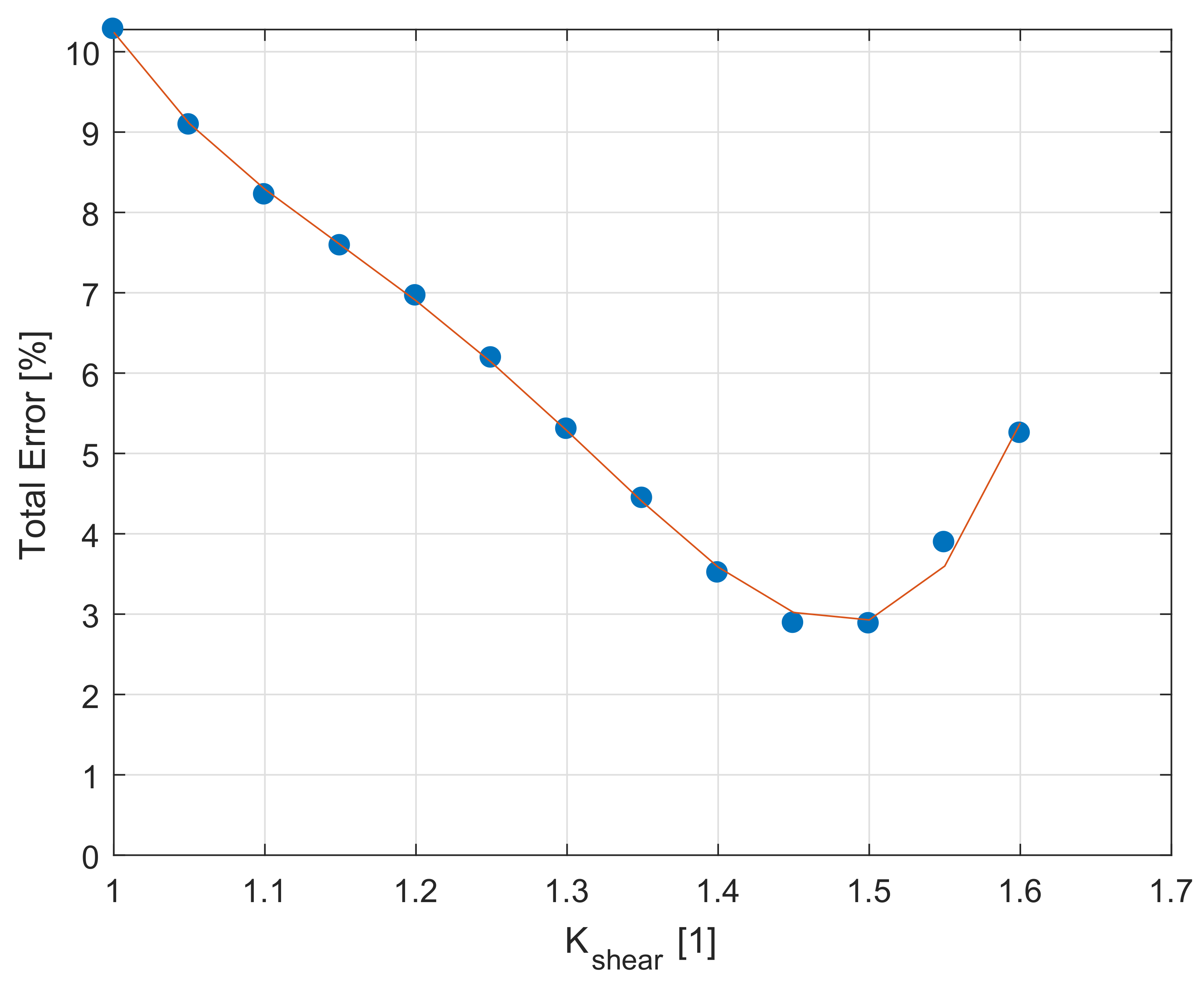
KShear = 1.50
C get PE components
call GETVRM('PE',ARRAY,JARRAY,FLGRAY,JRCD,JMAC,JMATYP,
+ MATLAYO,LACCFLA)
C EQPLAS
EQPLAS = ARRAY(7)
oEQPLAS = STATEV(iEQPLAS)
dEQPLAS = EQPLAS - oEQPLAS
C get PE
do K1=1,NTENS
oEPLAS(K1) = STATEV(iEPLAS-1+K1)
EPLAS(K1) = ARRAY(K1)
dEPLAS(K1) = EPLAS(K1) - oEPLAS(K1)
enddo
C get ALPHAv
do K1=1,NTENS
ALPHA1v(K1) = STATEV(iALPHA1v-1+K1)
ALPHA2v(K1) = STATEV(iALPHA2v-1+K1)
ALPHA3v(K1) = STATEV(iALPHA3v-1+K1)
oALPHAv(K1) = STATEV(iALPHAv-1+K1)
ALPHA1r(K1) = STATEV(iALPHA1r-1+K1)
ALPHA2r(K1) = STATEV(iALPHA2r-1+K1)
ALPHA3r(K1) = STATEV(iALPHA3r-1+K1)
oALPHAr(K1) = STATEV(iALPHAr-1+K1)
enddo
C get FLOW vector
if(dEQPLAS.gt.ZERO) then
do K1=1,NDI
FLOW(K1) = dEPLAS(K1)/dEQPLAS
enddo
do K1=NDI+1,NTENS
FLOW(K1) = dEPLAS(K1)/TWO/dEQPLAS
enddo
else
do K1=1,NTENS
FLOW(K1) = ZERO
enddo
endif
C RM
RM = STATEV(iRM)
oRM = RM
C dALPHAv
do K1=1, NDI
dALPHA1v(K1) = (TWO/THREE*C1*dEQPLAS*FLOW(K1) -
+ GAMMA1*ALPHA1v(K1)*dEQPLAS)/(ONE+GAMMA1*dEQPLAS)
dALPHA2v(K1) = (TWO/THREE*C2*dEQPLAS*FLOW(K1) -
+ GAMMA2*ALPHA2v(K1)*dEQPLAS)/(ONE+GAMMA2*dEQPLAS)
dALPHA3v(K1) = (TWO/THREE*C3*dEQPLAS*FLOW(K1) -
+ GAMMA3*ALPHA3v(K1)*dEQPLAS)/(ONE+GAMMA3*dEQPLAS)
ALPHAv(K1) = (ALPHA1v(K1)+dALPHA1v(K1)) +
+ (ALPHA2v(K1)+dALPHA2v(K1)) + (ALPHA3v(K1)+dALPHA3v(K1))
!dALPHAv(K1) = ALPHAv(K1)-oALPHAv(K1)
dALPHAv(K1) = dALPHA1v(K1) + dALPHA2v(K1) + dALPHA3v(K1)
enddo
do K1=NDI+1, NTENS
dALPHA1v(K1) = (TWO/THREE*C1*dEQPLAS*FLOW(K1) -
+ GAMMA1*KShear*ALPHA1v(K1)*dEQPLAS)/(ONE+GAMMA1*dEQPLAS)
dALPHA2v(K1) = (TWO/THREE*C2*dEQPLAS*FLOW(K1) -
+ GAMMA2*KShear*ALPHA2v(K1)*dEQPLAS)/(ONE+GAMMA2*dEQPLAS)
dALPHA3v(K1) = (TWO/THREE*C3*dEQPLAS*FLOW(K1) -
+ GAMMA3*KShear*ALPHA3v(K1)*dEQPLAS)/(ONE+GAMMA3*dEQPLAS)
ALPHAv(K1) = (ALPHA1v(K1)+dALPHA1v(K1)) +
+ (ALPHA2v(K1)+dALPHA2v(K1)) + (ALPHA3v(K1)+dALPHA3v(K1))
!dALPHAv(K1) = ALPHAv(K1)-oALPHAv(K1)
dALPHAv(K1) = dALPHA1v(K1) + dALPHA2v(K1) + dALPHA3v(K1)
enddo
do K1=1, NTENS
ALPHA1v(K1) = ALPHA1v(K1) + dALPHA1v(K1)
ALPHA2v(K1) = ALPHA2v(K1) + dALPHA2v(K1)
ALPHA3v(K1) = ALPHA3v(K1) + dALPHA3v(K1)
ALPHAv(K1) = ALPHA1v(K1) + ALPHA2v(K1) + ALPHA3v(K1)
enddo
C magALPHAv
magALPHAv = ZERO
do K1=1, NDI
magALPHAv = magALPHAv + ALPHAv(K1)**2
enddo
do K1=NDI+1, NTENS
magALPHAv = magALPHAv + TWO*ALPHAv(K1)**2
enddo
magALPHAv = sqrt(THREE/TWO*magALPHAv)
C G function
G = magALPHAv - RM
if(magALPHAv.gt.ZERO) then
do K1 = 1, NTENS
DirVec(K1)=ALPHAv(K1)/magALPHAv
enddo
else
do K1 = 1, NTENS
DirVec(K1) = ZERO
enddo
endif
C double dot product DDP
DDP = ZERO
do K1 = 1, NDI
DDP = DDP+DirVec(K1)*dALPHAv(K1)
enddo
do K1 = NDI+1, NTENS
DDP = DDP+TWO*DirVec(K1)*dALPHAv(K1)
enddo
C heaviside function of G
if (G.gt.ZERO) then
heavisideG = ONE
elseif (abs(G).lt.TOLER) then
heavisideG = ONE/TWO
else
heavisideG = ZERO
endif
C memory surface RM
dRM = heavisideG*abs(DDP)
RM = oRM + dRM
if (RM.lt.RMmin) then
RMused = RMmin
elseif (RM.gt.RMmax) then
RMused = RMmax
else
RMused = RM
endif
C RMR
RMR = STATEV(iRMR)
oRMR = RMR
do K1=1, NDI
dALPHA1r(K1) = (TWO/THREE*C1*dEQPLAS*FLOW(K1) -
+ GAMMA1*ALPHA1r(K1)*dEQPLAS)/(ONE+GAMMA1*dEQPLAS)
dALPHA2r(K1) = (TWO/THREE*C2*dEQPLAS*FLOW(K1) -
+ GAMMA2*ALPHA2r(K1)*dEQPLAS)/(ONE+GAMMA2*dEQPLAS)
dALPHA3r(K1) = (TWO/THREE*C3*dEQPLAS*FLOW(K1) -
+ GAMMA3*ALPHA3r(K1)*dEQPLAS)/(ONE+GAMMA3*dEQPLAS)
ALPHAr(K1) = (ALPHA1r(K1)+dALPHA1r(K1)) +
+ (ALPHA2r(K1)+dALPHA2r(K1)) + (ALPHA3r(K1)+dALPHA3r(K1))
!dALPHAr(K1) = ALPHAr(K1)-oALPHAr(K1)
dALPHAr(K1) = dALPHA1r(K1) + dALPHA2r(K1) + dALPHA3r(K1)
enddo
do K1=NDI+1, NTENS
dALPHA1r(K1) = (TWO/THREE*C1*dEQPLAS*FLOW(K1) -
+ GAMMA1*KShear*ALPHA1r(K1)*dEQPLAS)/(ONE+GAMMA1*dEQPLAS)
dALPHA2r(K1) = (TWO/THREE*C2*dEQPLAS*FLOW(K1) -
+ GAMMA2*KShear*ALPHA2r(K1)*dEQPLAS)/(ONE+GAMMA2*dEQPLAS)
dALPHA3r(K1) = (TWO/THREE*C3*dEQPLAS*FLOW(K1) -
+ GAMMA3*KShear*ALPHA3r(K1)*dEQPLAS)/(ONE+GAMMA3*dEQPLAS)
ALPHAr(K1) = (ALPHA1r(K1)+dALPHA1r(K1)) +
+ (ALPHA2r(K1)+dALPHA2r(K1)) + (ALPHA3r(K1)+dALPHA3r(K1))
!dALPHAr(K1) = ALPHAr(K1)-oALPHAr(K1)
dALPHAr(K1) = dALPHA1r(K1) + dALPHA2r(K1) + dALPHA3r(K1)
enddo
do K1=1, NTENS
ALPHA1r(K1) = ALPHA1r(K1) + dALPHA1r(K1)
ALPHA2r(K1) = ALPHA2r(K1) + dALPHA2r(K1)
ALPHA3r(K1) = ALPHA3r(K1) + dALPHA3r(K1)
ALPHAr(K1) = ALPHA1r(K1) + ALPHA2r(K1) + ALPHA3r(K1)
enddo
C magALPHAr
magALPHAr = ZERO
do K1=1, NDI
magALPHAr = magALPHAr + ALPHAr(K1)**2
enddo
do K1=NDI+1, NTENS
magALPHAr = magALPHAr + TWO*ALPHAr(K1)**2
enddo
magALPHAr = sqrt(THREE/TWO*magALPHAr)
C G function
G = magALPHAr - RMR
if(magALPHAr.gt.ZERO) then
do K1 = 1, NTENS
DirVecR(K1)=ALPHAr(K1)/magALPHAr
enddo
else
do K1 = 1, NTENS
DirVecR(K1) = ZERO
enddo
endif
C double dot product DDP
DDP = ZERO
do K1 = 1, NDI
DDP = DDP+DirVecR(K1)*dALPHAr(K1)
enddo
do K1 = NDI+1, NTENS
DDP = DDP+TWO*DirVecR(K1)*dALPHAr(K1)
enddo
C heaviside function of G
if (G.gt.ZERO) then
heavisideG = ONE
elseif (abs(G).lt.TOLER) then
heavisideG = ONE/TWO
else
heavisideG = ZERO
endif
C memory surface RMR
dRMR = heavisideG*abs(DDP)
RMR = oRMR + dRMR
if (RMR.lt.RMmin) then
RMRused = RMmin
elseif (RMR.gt.RMmax) then
RMRused = RMmax
else
RMRused = RMR
endif
C R
oR = STATEV(iR)
AR = CR*exp(ER*RMRused)
dR = AR*((EQPLAS+dEQPLAS)**BR-EQPLAS**BR)
R = oR + dR;
C PHIinfty
PhiInfty = AInfty*RMused**4 + BInfty*RMused**3 +
+ CInfty*RMused**2 + DInfty*RMused + EInfty
C Omega
OMEGA∼= AOmega+BOmega*(RMused)**-COmega
C PHIcyc
oPHIcyc = STATEV(iPHIcyc)
dPHIcyc = OMEGA*(PhiInfty-oPHIcyc)*DEQPLAS
PHIcyc = oPHIcyc + dPHIcyc
C PHI
PHI = PHI0 + PHIcyc
C save STATEV
STATEV(iEQPLAS) = EQPLAS
do K1=1,NTENS
STATEV(iEPLAS-1+K1) = EPLAS(K1)
STATEV(iALPHA1v-1+K1) = ALPHA1v(K1)
STATEV(iALPHA2v-1+K1) = ALPHA2v(K1)
STATEV(iALPHA3v-1+K1) = ALPHA3v(K1)
STATEV(iALPHAv-1+K1) = ALPHAv(K1)
STATEV(iALPHA1r-1+K1) = ALPHA1r(K1)
STATEV(iALPHA2r-1+K1) = ALPHA2r(K1)
STATEV(iALPHA3r-1+K1) = ALPHA3r(K1)
STATEV(iALPHAr-1+K1) = ALPHAr(K1)
STATEV(120+K1) = dALPHAv(K1)
enddo
STATEV(iR) = R
STATEV(iRM) = RM
STATEV(iRMR) = RMR
STATEV(iRMused) = RMused
STATEV(iRMRused) = RMRused
STATEV(iPHIcyc) = PHIcyc
STATEV(iPHI) = PHI
STATEV(iPhiInfty) = PhiInfty
STATEV(127) = SYIELD+R
STATEV(128) = DDP
C FIELD(1)
FIELD(1) = SYIELD+R
STATEV(iFIELD1) = FIELD(1)
C FIELD(2)
FIELD(2) = PHI
STATEV(iFIELD2) = FIELD(2)
RETURN
END
Appendix B.2. Material Parameters Definition in the Abaqus Input File
The example of material parameters definition in Abaqus input file:
*Material, name=Material-1
*Depvar
128
*Elastic
210000.0,0.3
*Plastic, dependencies=2, hardening=COMBINED, datatype=PARAMETERS,
number backstresses=3
** Material data as∼a∼function of FIELD1 and∼FIELD2 follows:
SYIELD,C1,GAMMA1,C2,GAMMA2,C3,GAMMA3,FIDEL1,FIELD2
%%
In the last material data line, the numeric values of material parameters are written. The material data line repeats for different values of variables and . Variables definitions are: , , , , , , , , . So, for presented material model, few material data lines can look like this:
** Material data as∼a∼function of FIELD1 and∼FIELD2 follows: ** ... 250.0,63399.70889,222.83539,9999.77788,1367.02686,2000.0,0.0,250.0,1.5 150.0,63399.70889,237.69108,9999.77788,1458.16199,2000.0,0.0,150.0,1.6 151.0,63399.70889,237.69108,9999.77788,1458.16199,2000.0,0.0,151.0,1.6 ** ...
References
- Halama, R.; Sedlák, J.; Šofer, M. Phenomenological Modelling of Cyclic Plasticity. In Numerical Modelling; Miidla, P., Ed.; IntechOpen: Rijeka, Croatia, 2012; pp. 329–354. [Google Scholar]
- Halama, R.; Fumfera, J.; Gál, P.; Kumar, T.; Makropulos, A. Modeling the Strain-Range Dependent Cyclic Hardening of SS304 and 08Ch18N10T Stainless Steel with a Memory Surface. Metals 2019, 9, 832. [Google Scholar] [CrossRef]
- Jiang, Y.; Zhang, J. Benchmark experiments and characteristic cyclic plastic deformation behavior. Int. J. Plast. 2008, 24, 1481–1515. [Google Scholar] [CrossRef]
- Facheris, G.; Janssens, K.G.F.; Foletti, S. Multiaxial fatigue behavior of AISI 316L subjected to strain-controlled and ratcheting paths. Int. J. Fatigue 2014, 68, 195–208. [Google Scholar] [CrossRef]
- Kim, C. Nondestructive Evaluation of Strain-Induced Phase Transformation and Damage Accumulation in Austenitic Stainless Steel Subjected to Cyclic Loading. Metals 2018, 8, 14. [Google Scholar] [CrossRef]
- Borodii, M.; Shukayev, S. Additional cyclic strain hardening and its relation to material structure, mechanical characteristics, and lifetime. Int. J. Fatigue 2007, 29, 1184–1191. [Google Scholar] [CrossRef]
- Jin, D.; Tian, D.J.; Li, J.H.; Sakane, M. Low-cycle fatigue of 316L stainless steel under proportional and nonproportional loadings. Fatigue Fract. Eng. Mater. Struct. 2016, 39, 850–858. [Google Scholar] [CrossRef]
- Xing, R.; Dunji, Y.; Shouwen, S.; Xu, C. Cyclic deformation of 316L stainless steel and constitutive modeling under non-proportional variable loading path. Int. J. Plast. 2019, 120, 127–146. [Google Scholar] [CrossRef]
- Srnec Novak, J.; Benasciutti, D.; De Bona, F.; Stanojevic, A.S.; De Luca, A.; Raffaglio, Y. Estimation of Material Parameters in Nonlinear Hardening Plasticity Models and Strain Life Curves for CuAg Alloy. IOP Conf. Ser. Mater. Sci. Eng. 2016, 119, 012020. [Google Scholar] [CrossRef]
- Benallal, A.; Marquis, D. Constitutive Equations for Nonproportional Cyclic Elasto-Viscoplasticity. J. Eng. Mater. Technol. 1987, 109, 326–336. [Google Scholar] [CrossRef]
- Tanaka, E. A nonproportionality parameter and a cyclic viscoplastic constitutive model taking into account amplitude dependences and memory effects of isotropic hardening. Eur. J. Mech. A/Solids 1994, 13, 155–173. [Google Scholar]
- Jiang, Y.; Sehitoglu, H. Modeling of cyclic ratchetting plasticity, part I: Development of constitutive relations. J. Appl. Mech. 1996, 63, 720–725. [Google Scholar] [CrossRef]
- ASTM Standard E606-92. Standard Practise for Strain-Controlled Fatigue Testing; ASTM International: West Conshohocken, PA, USA, 1998. [Google Scholar]
- Fumfera, J.; Halama, R.; Kuželka, J.; Španiel, M. Strain-Range Dependent Cyclic Plasticity Material Model Calibration for the 08Ch18N10T Steel. In Proceedings of the 33rd Conference with International Participation on Computational Mechanics, Špičák, Czech Republic, 6–8 November 2017. [Google Scholar]
- Abdel-Karim, M.; Ohno, N. Kinematic hardening model suitable for ratchetting with steady-state. Int. J. Plast. 2000, 16, 225–240. [Google Scholar] [CrossRef]
- Peč, M.; Šebek, F.; Zapletal, J.; Petruška, J.; Hassan, T. Automated calibration of advanced cyclic plasticity model parameters with sensitivity analysis for aluminium alloy 2024-T351. Adv. Mech. Eng. 2019, 11, 1–14. [Google Scholar] [CrossRef]
- Halama, R.; Pagáč, M.; Paška, Z.; Pavlíček, P.; Chen, X. Ratcheting Behaviour of 3D Printed and Conventionally Produced SS316L Material. In Proceedings of the ASME 2019 Pressure Vessels & Piping Conference PVP2019, San Antonio, TX, USA, 14–19 July 2019. Paper Number PVP2019-93384. [Google Scholar]
© 2019 by the authors. Licensee MDPI, Basel, Switzerland. This article is an open access article distributed under the terms and conditions of the Creative Commons Attribution (CC BY) license (http://creativecommons.org/licenses/by/4.0/).