Abstract
The thermal behavior of Li-ion cells is an important safety issue and has to be known under varying thermal conditions. The main objective of this work is to gain a better understanding of the temperature increase within the cell considering different heat sources under specified working conditions. With respect to the governing physical parameters, the major aim is to find out under which thermal conditions a so called Thermal Runaway occurs. Therefore, a mathematical electrochemical-thermal model based on the Newman model has been extended with a simple combustion model from reaction kinetics including various types of heat sources assumed to be based on an Arrhenius law. This model was realized in COMSOL Multiphysics modeling software. First simulations were performed for a cylindrical 18650 cell with a -cathode to calculate the temperature increase under two simple electric load profiles and to compute critical system parameters. It has been found that the critical cell temperature , above which a thermal runaway may occur is approximately , which is near the starting temperature of the decomposition of the Solid-Electrolyte-Interface in the anode at . Furthermore, it has been found that a thermal runaway can be described in three main stages.
1. Introduction
Lithium-ion batteries (LIB) have found a wide range of applications in many consumer products in the last 25 years. LIBs are used in cell phones, tablet and laptop computers as well as in electric (EV) or hybrid electric (HEV) driven vehicles. The size and the capacity of the batteries differs with the application. A battery used in an EV or HEV is much bigger than the one used for a cell phone. However the scale up of the batteries leads to a complexity of the physical phenomenona that do not play any significant role in single or small battery systems.
The occurrence of these physical phenomena are spread over a wide range of time and length scales, from the atomic level up to the heat transfer of the whole battery. The relation of these different phenomena to each other is of great importance, especially regarding the safety of the battery systems.
The usage of model-based investigations promises a theoretical understanding of battery physics even beyond the point that is possible using experiments. Due to their general structure, the behavior of batteries is strongly affected by the interaction of physics on varying length and time scales. In the last two decades, many approaches have been reported in literature starting with the work of Newman [1,2,3] based on the theory of porous electrodes [4]. This theory is based on a electrochemical description of diffusion dynamics and charge transfer kinetics of a battery and can give a forecast of the electric response of a cell in an intercalation electrode system. This model is adequate in small battery systems. In large formatted battery cells, however, the uniformity of the electrical potential along the current collectors in the cell composites is no longer given. Additionally due to the inhomogeneity of the distribution of the temperature field with respect to the cell geometry, thermal dynamics must also be taken into account.
As consequence an extended coupled electrochemical-thermal model must be considered. First thermal approaches for Lithium batteries are suggested by Newman and Pals [5,6,7] using an inhomogeneous heat equation , where the coupling of the thermal and electrochemical model is realized with the heat generation terms. This approach can be applied to single battery cells as well as to whole batteries [8,9,10,11,12]. In parallel the multi-scale and multi-domain character of the electrochemical model is developed [13,14] by using the mathematical theory of homogenization resp. the spatial averaging theorem [15]. Newer approaches are reported in the works of [16,17,18].
First, coupling between the multi-scale, multi-domain electrochemical-thermal model is introduced by [19,20,21] and is under development until now. A general short overview can be found in [22] and some current results in [23,24,25]. The purpose of this modeling approach is to gain a better understanding of the behavior of large LIB systems, because the transport of electrical current and heat must be considered on the length scales of the electrode particles up to the length scale of the cell composite, which is in general an anisotropic medium. One central point in the modeling of LIBs is the aspects of cell safety which corresponds to the thermal stability of a LIB. Several exothermic reactions can occur inside a cell during operation as its inner temperature increases. If the heat creation is larger than the dissipated heat in the surrounding space, this may cause heat to accumulate inside the cell and chemical reactions will be accelerated which yields in a further temperature increase until a thermal runaway is reached. In these terms, a thermal runaway describes a rapid temperature increase in a very short time interval of the typical order of and above [26].
This phenomenon can not be described with the mathematical models mentioned above. A first attempt to overcome this disadvantage is given in [27]. The heat equation is coupled with ordinary differential equations (ODEs), describing the temporal evolution of the concentration of the exothermic reactions based on an Arrhenius-type law. Spotnitz et al. [28,29] give a first PDE modeling of a thermal runaway including reaction kinetics. In [30,31,32], the electrochemical-thermal model is extended with reaction kinetics based on an ODE formulation. Some newer results can be found in [33,34,35]. In [33] an oven test and the influence of convection is investigated, while [34] is focused on a Lithium-Titanate Battery with a model similar as the one described in [33]. The PhD Thesis of Tanaka [35] gives a detailed insight in the modeling and simulation of a thermal runaway for different chemistry.
In Section 2 of this article a model to describe the thermal behavior of a LIB in general with all sub-models is introduced and reviewed. In Section 2.1, the thermal model is formulated and the important heat sources are identified. In the following subsections, the corresponding mathematical models behind the several heat sources are given. In Section 2.2, the abusive exothermic kinetic reactions leading to a thermal runaway are given in terms of mathematical combustion theory [36,37] followed by a simplification in Section 2.3. In Section 2.4, the electrochemical heat source is considered and the multi-scale, multi-domain electrochemical model of LIB’s [22,23], which is implemented in the Battery and Fuel Cell Module in COMSOL Multiphysics, is introduced. In the Section 3 some results simulated in COMSOL Multiphysics are shown. In Section 3.1, the model with and without exothermic contributions is compared, followed by the computation of the time, where the thermal runaway occurs in Section 3.2. Additionally a first coarse classification of the thermal runaway is given. In Section 3.3 the critical overall cell temperature, where above the thermal runaway occurs, is determined. Furthermore intervals for the convective heat transfer coefficient and environmental temperature are computed in this case. In the final section, we summarize our results and an outlook of possible future work is given.
2. Modeling the Thermal Behavior of a Lithium-Ion Battery
Since the interior of a LIB is separated from the environmental air due to the battery can, the cell can be considered as a closed system. Under working conditions, i.e., the cell is exposed to an electrical load, heat is generated inside the cell due to several electrochemical and chemical processes. If more heat can be dissipated to the environment than is generated inside the cell, the LIB works in a stable state with respect to the temperature. If more heat is generated inside the cell than can be dissipated to the environment the cell is in an unstable state with respect to the temperature, leading to a permanent temperature increase, that finally can end in a thermal runaway. The critical aspect in the case of thermal runaway is its relation to energy conservation. With the help of energy conservation, one is able to describe thermal characteristics like heat generation and heat dissipation. For our consideration we state the following assumptions with respect to the geometry of the LIB (cylindrical, pouch or prismatic):
- (1)
- In a certain (infinitesimal) time interval the cell is under constant charge, discharge or in relaxation.
- (2)
- The cell geometry resp. volume is constant, i.e., elastic processes and gas generation inside the cell are not considered.
- (3)
- Without loss of generality (W.l.o.g.) the emissivity , heat transfer coefficient h, the density , heat capacity and thermal conductivity are assumed to be constant in space and time.
2.1. The Energy Conservation
Neglecting heat convection inside the LIB, the general equation for the conservation of energy can be derived from Fourier’s Law as initial-boundary problem [36,37,38] with the parabolic differential equation:
for the temperature of the cell and the corresponding initial and boundary conditions:
In this framework is a spatial interior or surface point of the cell and is the time coordinate. denotes the environmental temperature, is the initial temperature profile inside the cell at and it is assumed that the initial temperature at the boundary of the cell coincides with the environmental temperature at . is the outward pointing normal vector. Ω denotes the interior of the battery cell, ∂Ω represent the boundary of the cell and the closure is the complete cell. Furthermore h is the heat transfer coefficient, ϵ the emissivity, the Stefan-Boltzmann constant, i.e., , the density of the cell, the heat capacity is and denotes the thermal conductivity.
In the inhomogeneity different heat sources are included. These contributions come from the heat generated by exothermic kinetic reactions, Joule and Ohmic heat and from reversible and irreversible thermodynamic effects:
For each contribution of an additional complete mathematical model must be formulated.
2.2. Identifying Heat Sources From Exothermic Reaction Kinetics Inside the Lithium-Ion Batteries
Exothermic reaction kinetics are closely related to thermal abuse mechanisms inside a LIB. Several exothermic chemical reactions can occur inside a battery as the temperature increases. These may generate heat, which accumulates inside the cell and accelerates the chemical reaction between the cell components, if the heat transfer to the surroundings is not sufficient [39], i.e., if the heat generation rate exceeds the dissipation rate. External conditions for a temperature rise can be external heating, over-charging or -discharging, high current charging, nail penetration, external short or others. In these cases, a thermal runaway can occur resulting in leak, smoke, gas venting, flames etc., which leads to a destruction of the cells. Several authors have given models to describe abuse behavior and thermal runaway. First attempts to describe the exothermic reaction kinetics are given by [27]. A simplified reaction-diffusion model is given in the works of [30,31,32]. The case of nail penetration is described in [40]. A catastrophe theoretic approach can be found [41], which is based on a simplified ODE model and is extended in [42]. To describe the abuse behavior including thermal runaway, one has to identify the main exothermic chemical reactions. Following [26,27,31,32,43] the general mechanism that leads to a thermal runaway can be described with respect to rising temperature in four steps as follows:
- (1)
- SEI decomposition reaction: At , in an exothermic reaction, the solid-electrolyte interface (SEI) decomposes.
- (2)
- Negative solvent reaction: At an exothermic reaction between the intercalated Li-ions and the electrolyte starts (NE).
- (3)
- Positive solvent reaction: For an exothermic reaction between the positive material and the electrolyte takes place under the evolution of oxygen inside the cell (PE).
- (4)
- Electrolyte decomposition: In a final exothermic reaction the electrolyte decomposes at (ELE).
The several temperatures may differ with the cell chemistry. For a - chemistry the corresponding temperatures are [32]: and . Other exothermic- or endothermic contributions are neglected in this work. For example exothermic reactions caused by a phase transition of from hexagonal to cubic crystal structure give a reaction enthalpy of typical 4– [44] in comparison to the SEI decompostion, where the enthalpy is between 250– [28]. Furthermore the produced oxygen during the phase change can lead to additional exothermic reactions with the electrolyte which can accelerate the thermal runaway [45].
A suitable theory to describe exothermic reaction kinetics is the mathematical theory of combustion [36,37]. Within this theory, if one is mainly interested in temperature dynamics, the usage of a so called solid fuel model is a possible approach. A Solid Fuel Model consists of the Equations (1)–(3) and an additional system of parabolic differential equations to describe the time-spatial evolution of the concentrations, the several constituents of the exothermic kinetic reactions with the corresponding initial and boundary equations. These equations may be derived from Fick’s Law of diffusion. In the following, we assume that the several exothermic reactions are independent from each other and are governed by a simple Arrhenius law. With and , we denote the spatial domain where the exothermic reaction took place, is the corresponding boundary and the closure. Then the i-th exothermic reaction can be written as:
Here is the initial concentration, is the diffusion coefficient, the stoichiometric coefficient. Then the exothermic heat sources can be computed assuming an Arrhenius-law:
where is the heat release in , the reaction rate in , the frequency factor in , the dimensionless reaction order, the activation energy in and R the universal gas constant, i.e., .
This gives the total exothermic heat source as:
2.3. Simplification of Combustion Model: The Constant Fuel Model
For our simulation the solid fuel model will be simplified to a constant fuel model [38,52] by neglecting all time-spatial dynamics of the concentrations , if one assumes that:
2.4. The Electrochemical Heat Source of a LIB and the Electrochemical Model
If one applies the thermal model described in last two sections to a LIB, this will coincide with a so called oven-trial for a Li-ion cell [31,32]. The cell is placed in a hot environment and the environmental temperature is increased with a specific profile. The cell is then heated only from the outside, if no current load is applied. If the environmental temperature is held constant and the cell is exposed to a current load, the cell will be heated from the inside. In addition to the exothermic heat contributions, additional electrochemical heat sources like Joule/Ohmic heating and reversible and irreversible effects will also occur. In summary these heat sources are given as
with
where I is the applied current profile in A, U the cell voltage and the equilibrium voltage of the cell in V. is the internal resistance of the LIB in Ω. The critical variable in the electrochemical heat source is the equilibrium voltage and derivation of the equilibrium voltage with respect to the temperature. In the Ohmic heat source, the internal resistance must be computed from the first partial derivative of the electric potential in the liquid and solid phase and the concentration of the Li-ions in the cell. These are additional variables to compute. These quantities must be computed with a separate mathematical model based on the porous electrode model developed by Newman [4]. This type of model has been under constant development in the last twenty years and describes a multi-scale multi-domain model (MSMD) to resolve the spatial-temporal electrochemical dynamics of a LIB with the Equations (1)–(3). The MSMD approach takes the physical and geometrical structure on different length scales and different geometrical domains into account. The general scheme is given in Figure 1. The three domains of interest and their inclusion in the LIB are identified (a) the particle domain; (b) the electrode domain and (c) the cell domain. To every domain an associated coordinate system taking into account the corresponding length scale and geometry is used.
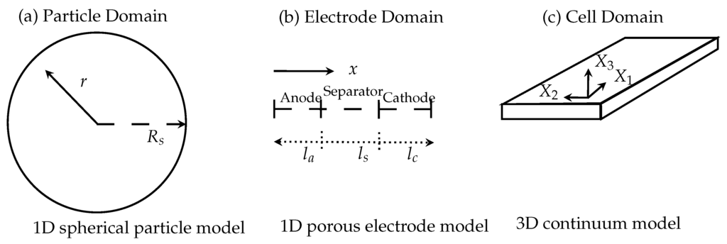
Figure 1.
Scheme of the several domain levels and their corresponding coordinate systems. (a) Particle domain; (b) electrode domain; (c) cell domain.
At the electrode-electrolyte interface charge transfer kinetics have to be solved. The transport of the Li-ions is modeled with a diffusion mechanism and the migration and diffusion of the Li-ions through the liquid electrolyte can be evaluated. The charge balances in the solid and liquid phase are also resolved in the corresponding domains, i.e., cathode, anode and separator. The model is able to predict the electrical behavior of a LIB cell for given electrical load. In this extended form with the Equations (1)–(3) the temperature-distribution is solved over the whole cell geometry. The electrochemical dynamics of a LIB can mathematically be described as coupled system of elliptic and parabolic differential equations for the concentration of the Li-ions and the electric potential in the electrochemical active domain . From the concentractions of the Li-ions and electrical potentials in the subdomains the corresponding heat sources in the Equations (14)–(17) have to be computed with a suitable homogenization using the spatial averaging theorem [15] from current densities and heat fluxes. This model is implemented in the Battery and Fuel Cell Module of COMSOL Multiphysics. A short review can be found in [22] and a more detailed review in [46].
3. Simulations
First simulation results using COMSOL Multiphysics Version 4.4 are given in this chapter. The model was implemented in the Battery and Fuel Cell Module of COMSOL Multiphysics. This module includes some predefined models of a LIB as described in the last section. The user defines his simulation problem including the concrete models, their coupling, the cell geometry, the simulation parameters and the spatial-temporal discretisation.
The purpose of this first simulation is to get a better insight in the thermal behavior of a LIB under normal and abuse conditions. The standard battery model in this module is not able to resolve thermal runaway. In the following the standard model is labeled as Model A. Therefore, an extension of this model with additional contributions is required. This extension is described in the last section together with the battery model and implemented in COMSOL Multiphysics in our already existing model in the most simple case first. This model is labeled as Model B in the following.
We consider a cylindrical 18650 cell with chemistry, i.e., in the COMSOL Multiphysics material database a anode, a cathode and as electrolyte with a salt is chosen. The internal spiral wounds are not resolved in this work, which means, that the geometric considerations will be restricted to the -plane. Only the additional heat sources are used to extend the temperature equation with additional heat sources (Constant fuel assumption) from the reaction-diffusion system of the exothermic reactions inside the LIB. These heat contributions are directly implemented with the electrochemical heat sources in the MSMD approach.
It is assumed, that a single LIB is placed in an Accelerating Rate Calorimeter (ARC) and the environment of the LIB in the ARC is filled with air. Experimental measurements inside the ARC gave typical values for h in the range of . During the simulations the convective heat transfer coefficient h is varied in the interval of . This setup represents adiabatic conditions for . The non adiabatic conditions with positive h describes the free flow of gases and steams for in general, stationary gases and air in the environment are described by h in the interval [47]. Therefore only natural convection is considered in this work.
In a cylindrical geometry, the equations for the particle and electrode domain model remains unchanged. Only on cell domain the corresponding equations for the potentials at the current collector and the temperature field have to be reformulated in cylindrical coordinates in the plane, i.e., :
The initial and boundary conditions of the temperature field T are given in the Equations (2) and (3). Since the electrodes and the separator possess a porous structure, where the pores are filled with the electrolyte, the thermal parameter in the heat Equation (19) have to be considered as an effective parameter. Therefore in each of the three porous domains the total value of the thermal parameter is computed with a mixture formula containing the parameter value of the corresponding solid phase and the liquid electrolyte. Then the effective thermal conductivity (radial-, z- direction) , density and heat capacity are given as follows [30]:
where denotes the index set to the corresponding parameter in cathode, anode, separator and current collector.
The last four equations can be regarded as special cases from corresponding formulas of the spiral geometry restricted to the plane [48,49]. Therefore, this thermal model can be considered as a serial thermal network in direction and a parallel thermal network in direction. With the parameters from Table A1 in the appendix, the corresponding effective parameters are given in Table 1. In this table, the effective parameters are compared with parameters given in literature [50,51].

Table 1.
Effective thermal parameter used in simulation in comparison with effective thermal parameter given in literature.
The main physical parameters of the simulation for both models can be found in Table A1 and in Table A2 in the appendix. The additional simulation parameters of the exothermic reaction in Model B for the abuse contributions are taken from [30,31].
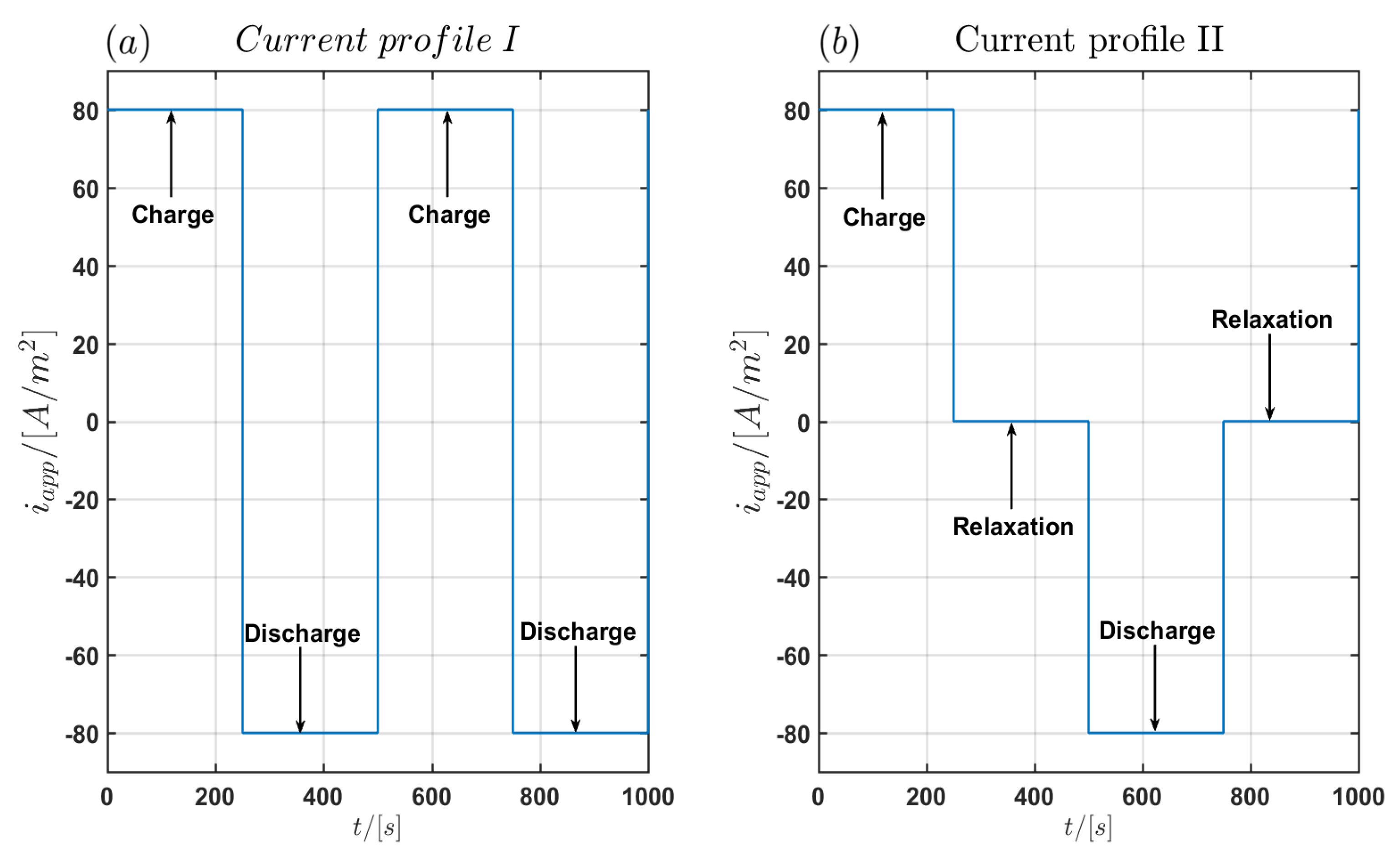
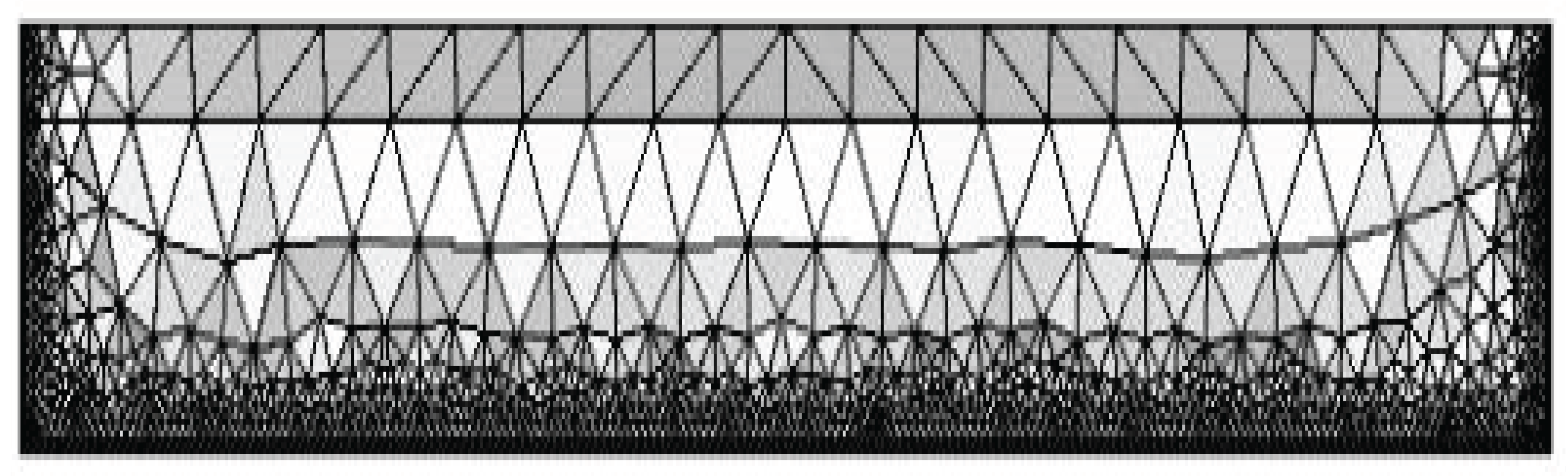
The simulations were performed with the two current load profiles with a constant current density of as seen in Figure 2. In the first profile labeled Profile I shown in Figure 2a there are no relaxation periods between the charging and discharging pulses with duration of each. In the second profile (Profile II) relaxation periods of between charging and discharging pulses are used as shown in Figure 2b. A complete current cycle lasts and . The maximal simulation time is and . For the time integration in COMSOL Multiphysics, a BDF integration scheme is chosen with a minimum order of 1 and a maximum order of 5 using a variable step size with a maximum time step of and an absolute tolerance of . Since the spatial discretisation in COMSOL Multiphysics is based on the FEM method, we have used an adaptive spatial discretisation in the three models of the particle domain, the electrode domain and the cell domain respectively. The model of the particle domain is solved automatically in the battery module of COMSOL Multiphysics. Therefore only a spatial discretisation for the electrode domain and the cell domain is required. In the electrode domain, the maximum element size in the discretisation is chosen as In total the discretisation contains 168 elements. Quadratic basis functions were chosen for the one-dimensional finite element discretisation in the electrode domain. In the cell domain the spatial discretisation is performed in the -plane using 2266 triangular elements with the element size in the interval and quadratic basis functions. The FEM discretisation is shown in Figure 3.

Figure 2.
(a) First of the current load profile I without relaxation times and (b) of the current load profile II with relaxation times of 250 s between charging and discharging pulses.
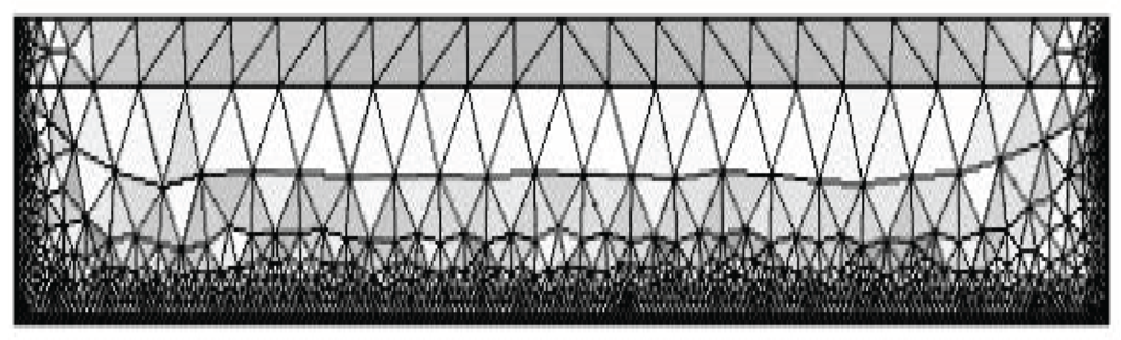
Figure 3.
Meshing of a cylindrical 18650 cell.
The main purpose of this section is to compute the overall mean cell temperature, below which the LIB shows normal behavior and above which the cell shows a thermal runaway with respect to some system parameters like the environmental temperature or the convective heat transfer coefficient. Furthermore, critical values for such parameters will be computed from the simulations and a first coarse classification of the thermal runaway will be given.
3.1. Model Comparison
In a first step Model A and Model B are compared under normal and abusive conditions with Profile (I). The following three cases are considered:
- (1)
- : In this case the LIB is unable to dissipate any generated heat to the environment. Therefore, a thermal runaway will always occur after a sufficiently large time.
- (2)
- h positive and a thermal runaway occurs after a sufficiently large time: In this case, more heat is generated inside the LIB, as can be dissipated to the environment.
- (3)
- h positive and no thermal runaway occurs after a sufficiently large time: In this case the generated heat can be dissipated completely to the environment.
The first case coincides with adiabatic boundary conditions while the other two cases coincide with isoperibolic boundary conditions. Additionally for this comparison an environmental temperature of is chosen as a representative temperature in the interval of . This temperature coincides with the minimum temperature where stable environmental conditions can be adjusted in the ARC. As corresponding convective heat transfer coefficients the values are chosen. The spatial averaged mean cell temperature of all interior points is considered W.l.o.g. the overall mean cell temperature can be replaced by the mean temperature of the cell surface or the temperature at an arbitrary interior point of the cell. , i.e.,
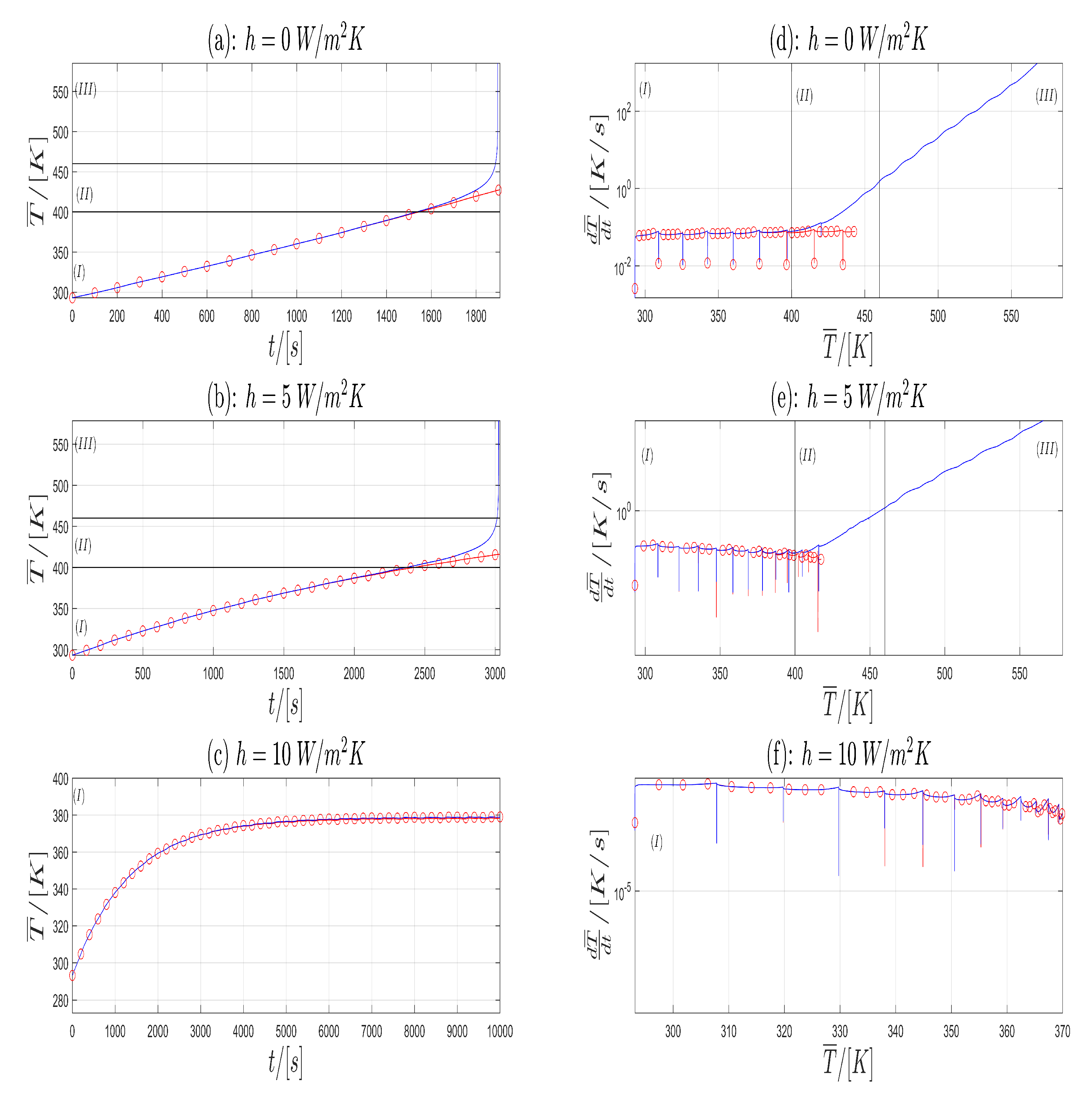
Since the simulation results are stored in a non-equidistant time grid, the mean temperature is interpolated to an equidistant time grid with using splines with Matlab® 2015b. In Figure 4a–c the Time- Temperature plots for Model A (blue) and Model B (red) are shown with respect to . In Figure 4d–f the corresponding Temperature-Heating Rate plots are given on a semi-logarithmic scale. From Figure 4 one can see that in (a) and (b) both models shows similar behavior until resp. . The corresponding cell temperature is approximately (Lower horizontal line in (a), (b), first vertical line in (d), (e)). This temperature is near to the start temperature of SEI decomposition, which is given in [26] to . After this time Model B exhibits a greater increase in temperature as Model A. Finally, the simulation of Model B shows a blow-up in solution which corresponds to a thermal runaway in a LIB. For , the reaction for the electrolyte decomposition starts [26]. This is marked with the upper horizontal line in (a), (b) and the second vertical line in (d), (e) in Figure 4. The corresponding heating rate is which correspond very well with the start of the thermal runaway given in [26] with . In (c), both models have no significant difference in their time evolution of the temperature and the both solutions remain bounded. Therefore, in the graphs (a), (b) and (d), (e) of Figure 4 one can split the time evolution of the temperature in the three zones (I),(II) and (III).
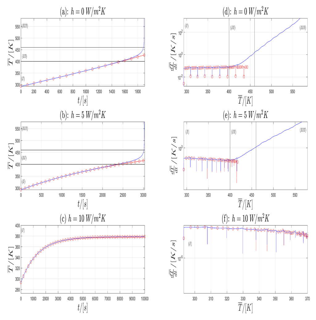
Figure 4.
-plot (a–c) and corresponding plot (d–f) for the Model A (blue) and Model B (red) and three different h values.
First consider the plots (a) and (b) of Figure 4. In Zone (I) the cell shows a normal behavior. In this zone, the heat generation is governed by the electrochemical, Joule and Ohmic heat contributions. Exothermic contributions are negligible. In Zone (II), the cell temperature is high enough, so that the exothermic heat contributions are no longer negligible. This zone can be considered as an intermediate zone or the onset of the thermal runaway. In Zone (III), the exothermic heat contributions are dominant and thermal runaway takes place. Electrochemical heat contributions can be neglected in Zone (III).
Next consider in Figure 4 in the plots (d), (e), (f) the corresponding Temperature-Heating Rate trajectory. Since the current profiles Profile I and Profile II are of a rectangular shape, the first derivative will be a piecewise continuous function with discontinuities at the time, where the current profiles jumps. Therefore, we consider in the sense of distributions. At the time of the discontinuities one has to take the limit from right and left to get a derivation from left and right.
The graphs in (d) and (e) can be separated into three zones again (Vertical black lines). In the first zone (I) Model A and Model B show similar behavior with an increase in the mean cell temperature while the heating rate remains almost constant or has a small decrease with respect to some outlier points. These points coincide with the time, where the current profile jumps from the charging state to the discharging state and vice versa. At the end of zone (I) in Model B, the heating rate begins to rise. This is justified due to heat contribution of the exothermic reaction, which is no longer negligible. The general shape of the curve from Model B remains unchanged. This is the transition to zone (II). In the zones (II) and (III) one observes an increase in temperature T and an increase in the heating rate , which is justified in the accelerating of the exothermic reactions. The transition from zone (II) to (III) is reached, when the heating rate exceeds the critical value of [26]. The corresponding temperatures are computed from the plots (d) and (e) in Figure 4 as the intersection the horizontal black line with the graph of Model B (red). This result is compared with the upper black line in the plots (a) and (b) with the graph of Model B (red). The results are given in the last column in Table 2. Next, we compare our simulation results for Model B with the experimental results from Abraham et al. [26]. In their work, the thermal abuse of a 18650 cell with a chemistry is considered. The time evolution of the temperature is also grouped into three zones. A comparison between the experimental results from [26], the results given in [32] and our simulation results is given in Table 2. From a physical point of view one can interpret the zones (I)–(III) as follows: If the curve remains in zone (I) and stays below certain temperature values the cell works in safe conditions. If the -curve changes to zone (II) thermal runaway starts, and both the heating rate and temperature rise. In zone (III) the heating rate exceeds a critical heating rate value. This is the thermal runaway, in which the heating rate tends to infinity. In Figure 4c,f both models stay in zone (I), no thermal runaway occurs and no significant difference is to be observed in both models.
Table 2.
Classification of the time evolution of the temperature during thermal runaway.
In summary one can see the difference between Model A and Model B due to the exothermic heat sources in the temperature development over the time and corresponding heating rate. Furthermore Model B gives a good agreement with experimental results from literature [26,32] and a coarse classification of the time evolution of a thermal runaway event has been made. This topic will be considered in more detail in a subsequent publication.
3.2. Computing the Thermal Runaway Time
In this and the following section only Model B is considered. The environmental temperature is and steps of were employed. In the simulations for each , the heat transfer coefficient h is in the interval and the emissivity is equal to . The time required for thermal runaway to occur with respect to the environmental temperature and convective heat transfer coefficient is computed in the simulation. For this purpose, the term Thermal runaway time has to be precisely defined.
Definition 1.
The Thermal Runaway Time of a Lithium ion cell is defined as the time, at which the heating rate exceeds a predefined threshold i.e., such that:
for sufficiently high cell temperatures.
For an equidistant time grid of , the heating rate is approximated by the Equation (26).
The threshold is chosen here as:
The thermal runaway time is chosen as the time at which the condition is achieved.
In Table 3 and Figure 5 the time for the current profiles (I) and (II) is given with respect to and h. The following two cases are considered:
Table 3.
Thermal runaway time with respect to heat transfer coefficient h and the environment al temperature . (a) Profile (I), (b) Profile (II).
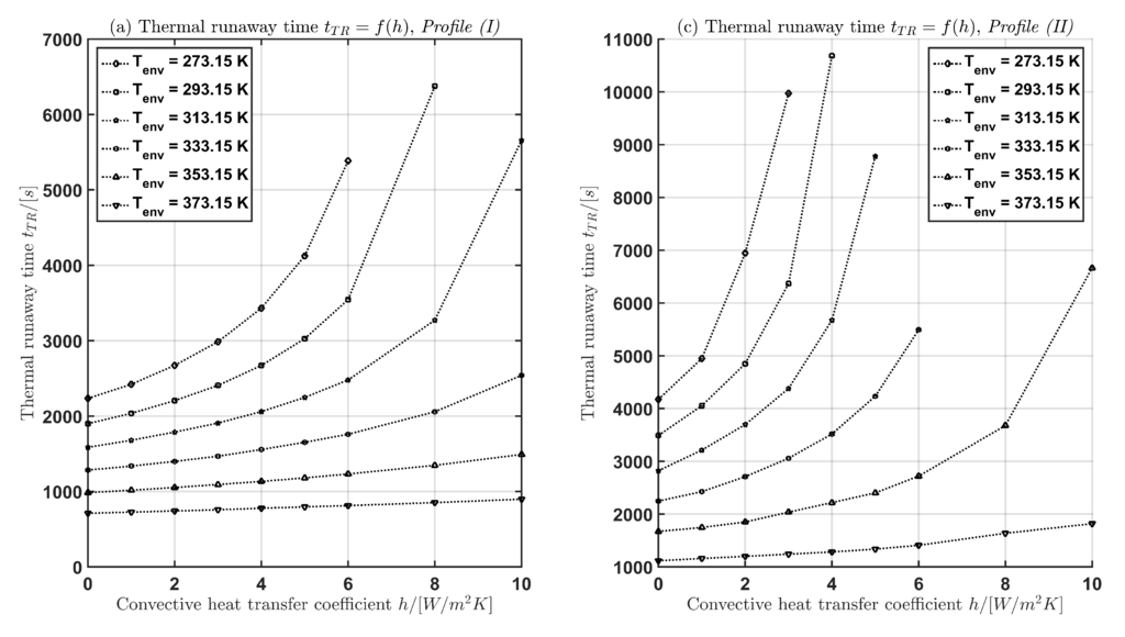
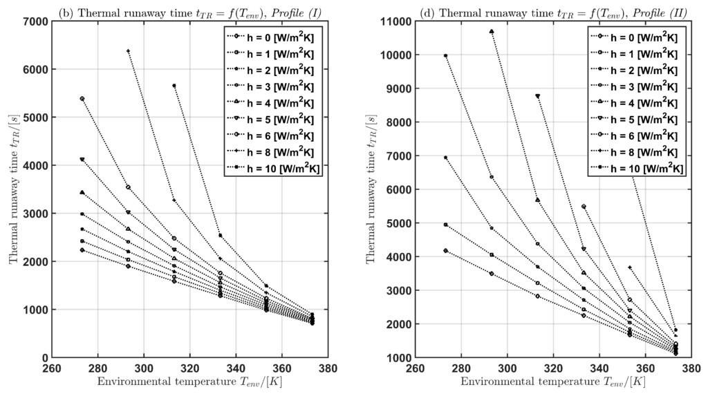
Figure 5.
Thermal runaway time as function of the convective heat transfer coefficient h (a),(b) and as function of the environmental temperature (c),(d) for both current profiles Profile (I) and Profile (II).
In case (1) for a fixed environmental temperature, the thermal runaway time increases with increasing convective heat transfer coefficient h. In case (2) for a fixed convective heat transfer coefficient, the thermal runaway time decreases with increasing environmental temperature.
3.3. Critical parameter intervals
In the last section the thermal runaway time was computed. In this section the time evolution of the mean cell temperature was computed, again in the cases (1) and (2) from Section 3.2. The aim is to calculate the critical mean cell temperature with respect to the parameter and h in the sense, that below the critical temperature the LIB is under safe conditions and above the LIB will show a thermal runaway. Therefore, multiple simulations of the current profiles (I) and (II) are performed. In all simulations the environmental temperature is in the interval and the convective heat transfer coefficient h is in the interval . The purpose of the simulations was to compute numerically approximately intervals for the critical environmental temperature and the critical convective heat transfer h, analog to the cases (1) and (2) from Section 3.2 for fixed environmental temperature and variable heat transfer coefficient h (case(1)) and vice versa (case (2)). The critical parameter intervals are determined with a bisection procedure, where successive the intervals of the parameter under investigations is shrinking with respect to the fact, if a thermal runaway in the simulation occurs or not.
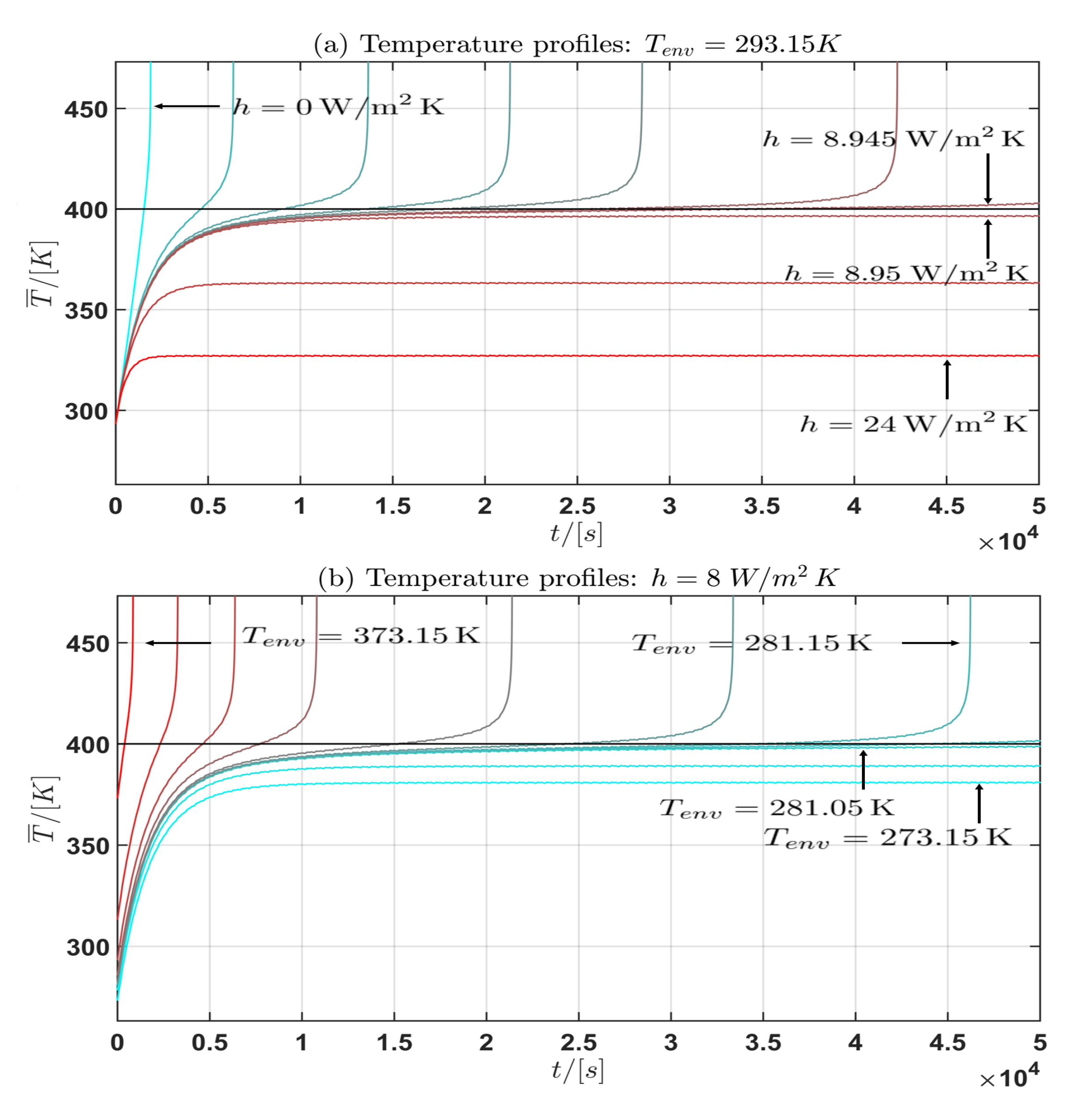
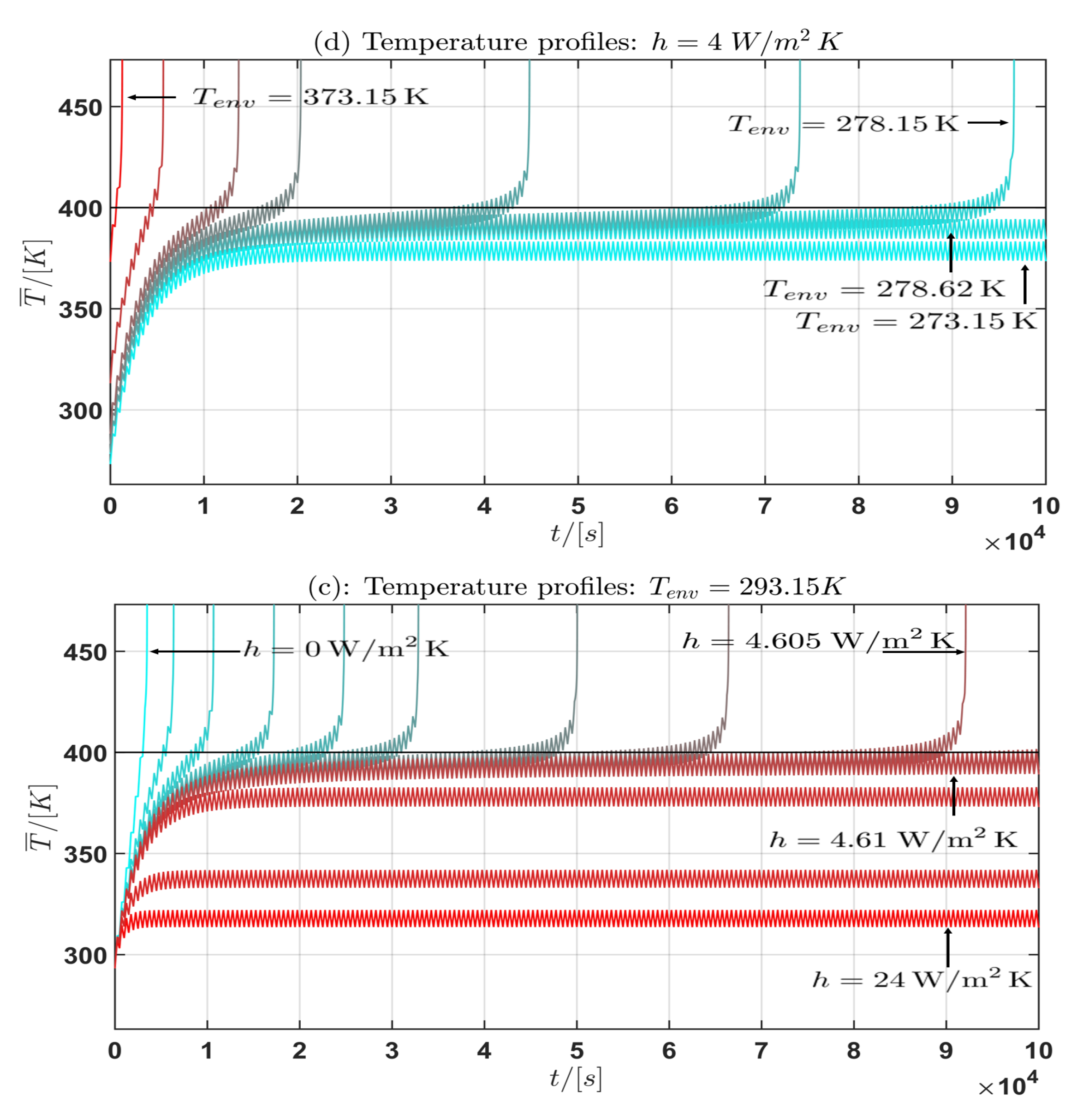
The results are plotted in the Figure 6 and Figure 7. In the subplots (a) and (c) for , the convective heat transfer coefficient is varied in the interval for the current profiles (I) and (II). In the subplots (b) and (d), the environmental temperature is varied over the interval for and for the current profiles (I) and (II). In Table 4 some approximate intervals for the critical parameter are given.
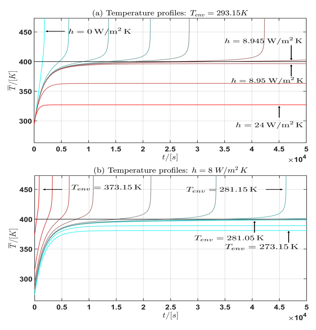
Figure 6.
Profile (I): Temperature profile for the mean cell temperature : (a) fixed, h varied; (b) h fixed, varied.

Figure 7.
Profile (I): Temperature profile for the mean cell temperature : (a) fixed, h varied; (b) h fixed, varied.
Table 4.
Critical parameter intervals: Profile (I) (a) fixed, (b) h fixed, Profile (II) (c) fixed, (d) h fixed.
Moreover from the temperature curves of the mean cell temperature in the Figure 6 and Figure 7 the critical mean cell temperature is . Since the development of a complete mathematical theory is far beyond the scope of this work an extension of the theories of Semenov [52] and Frank-Kamenetskii [38] and the corresponding critical parameter will be considered in future work. In summary the following general statement can be given from the observation of the simulation results:
Statement 1.
Let be a the asymptotic temperature profile if the limit exists. Then the following holds:
- (a) If the environmental temperature is constant and fixed and the convective heat transfer coefficient h is allowed to vary, then with:
- -
- -
- (b) If the convective heat transfer coefficient h is constant and fixed and the environmental temperature is allowed to vary, then with:
- -
- -
If or is bounded then it is (almost) constant for the current profile (I) and periodic for the current profile (II).
4. Conclusions and Outlook
In this work a model for the simulation of a thermal runaway in LIBs for a given current profile was introduced. The thermal model was extended with additional heat sources coming from several exothermic reactions inside the LIB due to the constant fuel assumption. In the electrochemical part of our model we took the length scales for the essential dynamics into account. This results in a coupled system of elliptic and parabolic partial differential equations on the particle, the electrode and the cell domain respectively. The coupling of the equations of the particle domain with the the equations of the electrode domains, as well as the the equations of the electrode domain with the equations of the cell domain is solved with suitable homogenization procedures using the spatial averaging theorem which is based on the assumption of spatial homogeneity. Despite the fact that the advantages of this model in the spatial resolution are not used in this work, it is the intention of the authors to consider spatial localized effects in the dynamics of a thermal runaway in future work with this model. In this work we show the difference between the old model Model A and the model with additional contributions for exothermic reactions Model B. Furthermore, we have shown that Model B is able to show a thermal runaway in contrary to Model A. We defined and computed the thermal runaway time with respect to some system parameters as well as the critical cell temperature which can be interpreted as a marker for the cell stability with respect to thermal dynamics. Furthermore, a coarse classification of thermal runaway is given with the Model B. In summary, in these simulations, which were performed using COMSOL Multiphysics, we have shown that these additional exothermic terms in the numerical FEM model can resolve such phenomena for a specific current load profile. Due to the constant fuel assumption, this model is not able to resolve the decay period of a thermal runaway after all fuel is consumed. Also, the change in the amount of fuel is not considered in this model. For future work, this first model describing the thermal runaway of LIB’s will be improved by skipping the constant fuel assumption. A detailed consideration of the underlying battery chemistry and corresponding exothermic reaction kinetics is planned in addition to determining a criteria to predict a thermal runaway with the information given by the simulations. Furthermore, it is planned to compare the simulations of this model with experimental results in a future work.
Acknowledgments
This R&D project is partially funded by the Federal Ministry for Education and Research (BMBF) within the framework “IKT 2020 Research for Innovations” under the grant 16N12515 and is supervised by the Project Management Agency VDI | VDE | IT.
We acknowledge support by Deutsche Forschungsgemeinschaft and Open Access Publishing Fund of Karlsruhe Institute of Technology.
Author Contributions
Andreas Melcher: Modeling the thermal runaway, Performing the simulation and data evaluation; Carlos Ziebert: Electrochemical and thermal modeling; Magnus Rohde: Electrochemical modeling, thermal modeling, first simulations; Hans Jürgen Seifert: Electrochemical, thermal modeling
Conflicts of Interest
The authors declare no conflict of interest.
Appendix: Simulation Parameters
Table A1.
Simulation parameters.
| Initial values | |||
|---|---|---|---|
| Li-concentration neg. solid phase | Li-concentration pos. solid phase | ||
| Initial temperature | Li-concentration liquid phase | ||
| Li-diffusivity | |||
| Neg. solid phase | Pos. solid phase | ||
| Volume frcation | |||
| Neg. solid phase | Pos. solid phase | ||
| Neg. liquid phase | Pos. liquid phase | ||
| Maximal concentration | |||
| Neg. solid phase | Pos. solid phase | ||
| Thermal conductivity | |||
| Neg. electrode | Pos. electrode | ||
| Neg. current collector | Pos. current collector | ||
| Density | |||
| Neg. electrode | Pos. electrode | ||
| Neg. current collector | Pos. current collector | ||
| Particle radius | |||
| Neg. particle | Pos. particle | ||
| Reaction rate coefficient | |||
| Neg. electrode | Pos. electrode | ||
| Neg. electrode | Pos. electrode | ||
| Neg. current collector | Pos. current collector | ||
| Separator | |||
| Density | Thermal conductivity | ||
| Heat capacity | |||
| Battery geometry | |||
| Radius | Height | ||
| Mandrel radius | |||
| Cell thickness | Thickness battery canister | ||
| Thickness neg. current collector | Thickness pos. current collector | ||
| Length pos./neg. electrode | Length separator | ||
Table A2.
Exothermic simulation parameters.
| Reaction Heat | Frequency | Activation Energy | Volume Content | |
|---|---|---|---|---|
| factor | ||||
| SEI reaction | ||||
| Neg. solvent reaction | ||||
| Pos. solvent reaction | ||||
| Electrolyte decomp. |
References
- Doyle, M.; Fuller, T.F.; Newman, J. Modeling Galvanostatic Charge and Discharge of the Lithium/Polymer/ Insertion Cell. J. Electrochem. Soc. 1993, 140, 1526–1533. [Google Scholar] [CrossRef]
- Fuller, T.F.; Doyle, M.; Newman, J. Simulation and Optimization of the Dual Lithium Ion Insertion Cell. J. Electrochem. Soc. 1994, 141, 1–10. [Google Scholar] [CrossRef]
- Doyle, M.; Newman, J. Comparison of the Modeling Predictions with Experimental Data from Plastic Lithium Ion Cells. J. Electrochem. Soc. 1996, 143, 1890–1903. [Google Scholar] [CrossRef]
- Newman, J.; Tiedemann, W. Porous-Electrode Theory with Battery Applications. AIChE J. 1975, 21, 25–41. [Google Scholar] [CrossRef]
- Newman, J.; Tiedemann, W. Temperature Rise in a Battery Module with Constant Heat Generation. J. Electrochem. Soc. 1995, 142, 1054–1057. [Google Scholar] [CrossRef]
- Pals, C.R.; Newman, J. Thermal modeling of Lithium/Polymer Battery, I. Discharge Behavior of a Single Cell. J. Electrochem. Soc. 1995, 142, 3274–3281. [Google Scholar] [CrossRef]
- Pals, C.R.; Newman, J. Thermal modeling of Lithium/Polymer Battery, II. Temperature Profiles in a Cell Stack. J. Electrochem. Soc. 1995, 142, 3282–3288. [Google Scholar] [CrossRef]
- Al Hallaj, S.; Maleki, H.; Hong, J.S.; Selman, J.R. Thermal modeling and design considerations of lithium-ion batteries. J. Power Sour. 1999, 83, 1–8. [Google Scholar] [CrossRef]
- Chen, S.C.; Wan, C.C.; Wang, Y.Y. Thermal analysis of lithium-ion batteries. J. Power Sources 2005, 140, 111–124. [Google Scholar] [CrossRef]
- Inui, Y.; Kobayashi, Y.; Watanabe, Y.; Watase, Y.; Kitamura, Y. Simulation of temperature distribution in cylindrical and prismatic lithium ion secondary batteries. Energy Convers. Manag. 2007, 48, 2103–2109. [Google Scholar] [CrossRef]
- Zhu, C.; Li, X.; Song, L.; Xiang, L. Development of the theoretically based thermal model for lithium ion battery pack. J. Power Sources 2013, 223, 155–164. [Google Scholar] [CrossRef]
- Hu, J.; Tao, L.; Jing, L. Temperature Field Analysis and Thermal Dissipation Structure Optimization of Lithium-ion Battery Pack in PEVs. Res. J. Appl. Sci. Eng. Technol. 2014, 7, 62–71. [Google Scholar]
- Wang, C.Y.; Gu, W.B.; Liaw, B.Y. Micro-Macroscopic Coupled Modeling of Batteries and Fuel Cells. I. Model Development. J. Electrochem. Soc. 1998, 145, 3407–3417. [Google Scholar] [CrossRef]
- Gu, W.B.; Wang, C.Y.; Liaw, B.Y. Micro-Macroscopic Coupled Modeling of Batteries and Fuel Cells. II.Application to Nickel Cadmium and Nickel-Metal Hybride Cells. J. Electrochem. Soc. 1998, 145, 3418–3427. [Google Scholar] [CrossRef]
- Howes, F.A.; Whitaker, S. The Spatial Averaging Theorem Revisited. Chem. Eng. Sci. 1985, 40, 1387–1392. [Google Scholar] [CrossRef]
- Latz, A.; Zausch, J.; Iliev, O. Modeling of Species and Charge Transport in Li-Ion Batteries Based on Non-equilibrium Thermodynamics; Dimov, I., Dimova, S., Kolkovska, N., Eds.; NMA 2010, LNCS 6046; Springer: Berlin, Germany, 2011; pp. 329–337. [Google Scholar]
- Richardson, G.; Denault, G.; Please, C.P. Multiscale modeling and analysis of lithium-ion battery charge and discharge. J. Eng. Math. 2012, 72, 41–72. [Google Scholar] [CrossRef]
- Landstorfer, M.; Jacob, T. Mathematical modeling of intercalation batteries at the cell level and beyond. Chem. Soc. Rev. 2013, 42, 3234–3252. [Google Scholar] [CrossRef] [PubMed]
- Gu, W.B.; Wang, C.Y. Thermal-Electrochemical Modeling of Battery Systems. J. Electrochem. Soc. 2000, 147, 2910–2922. [Google Scholar] [CrossRef]
- Wang, C.Y.; Srinivasan, V. Computational battery dynamics (CBD)-electrochemical/thermal coupled modeling and multi-scale modeling. J. Power Sources 2002, 110, 364–376. [Google Scholar] [CrossRef]
- Kumaresan, K.; Sikha, G.; White, R.E. Thermal Model for Lion-Ion Cell. J. Electrochem. Soc. 2008, 155, A164–A171. [Google Scholar] [CrossRef]
- Cai, L.; White, R.E. Mathematical modeling of lithium ion battery with thermal effects in COMSOL Inc. Multiphysics (MP) software. J. Power Sources 2011, 196, 5985–5989. [Google Scholar] [CrossRef]
- Kim, G.H.; Smith, K.; Lee, K.J.; Santhanagopalan, A.P. Multi-Domain Modeling of Lithium-Ion Batteries Encompassing Multi-Phyiscs in Varied Length Scales. J. Electrochem. Soc. 2011, 158, A955–A969. [Google Scholar] [CrossRef]
- Guo, M.; Kim, G.H.; White, R.E. A three-dimensional multi-physics model for a Li-ion battery. J. Power Sources 2013, 240, 80–94. [Google Scholar] [CrossRef]
- Lee, K.J.; Smith, K.; Pesaran, A.; Kim, G.H. Three dimensional thermal-, electrical, and electrochemical-coupled model for cylindrical wound large format lithium-ion batteries. J. Power Sources 2013, 241, 20–32. [Google Scholar] [CrossRef]
- Abraham, D.P.; Roth, E.P.; Kostecki, R.; McCarthy, K.; MacLaren, S.; Doughty, D.H. Diagnostic examination of thermally abused high-power lithium-ion cells. J. Power Sources 2006, 161, 648–657. [Google Scholar]
- Hatchard, T.D.; MacNeil, D.D.; Basu, A.; Dahn, J.R. Thermal Model of Cylindrical and Prismatic Lithium-Ion Cells. J. Electrochem. Soc. 2001, 148, A755–A761. [Google Scholar] [CrossRef]
- Spotnitz, R.; Franklin, J. Abuse behavior of high-power, lithium-ion cells. J. Power Sources 2003, 113, 81–100. [Google Scholar] [CrossRef]
- Spotnitz, R.M.; Weaver, J.; Yeduvaka, G.; Doughty, D.H.; Roth, E.P. Simulation of abuse tolerance of lithium-ion battery packs. J. Power Sources 2007, 163, 1080–1086. [Google Scholar] [CrossRef]
- Kim, G.H.; Pesaran, A.; Spotnitz, R. A three-dimensional thermal abuse model for lithium-ion cells. J. Power Sources 2007, 170, 476–489. [Google Scholar] [CrossRef]
- Peng, P.; Sun, Y.; Jiang, F. Thermal analyses of LiCoO2 lithium-ion battery during oven tests. Heat Mass Transf. 2014, 50, 1405–1416. [Google Scholar] [CrossRef]
- Peng, P.; Sun, Y.; Jiang, F. Numerical simulations and thermal behavior analysis for oven thermal abusing of LiCoOO2 lithium-ion battery. CIESC J. 2014, 65, 647–657. [Google Scholar]
- Lopez, C.F.; Jeervarajan, J.A.; Mukherjee, P.P. Characterizarion of Lithium-Ion Battery Thermal Abuse Behavior Using Experimental and Computational Analysis. J. Electrochem. Soc. 2015, 162, A2163–A2173. [Google Scholar] [CrossRef]
- Chen, M.; Sun, Q.; Wu, K.; Liu, B.; Peng, P.; Wang, Q. A Thermal Runaway Simulation on a Lithium Titanate Battery and Battery Module. Energies 2015, 8, 490–500. [Google Scholar] [CrossRef]
- Tanaka, N. Modeling and Simulation of Thermo-Electrochemistry of Thermal Runaway in Lithium-Ion Batteries. Ph.D. Thesis, University of Stuttgart, Stuttgart, Germany, 2015. [Google Scholar]
- Bebernes, J.; Eberly, D. Mathematical Problems from Combustion Theory; Applied Mathematical Sciences Volume 83, Springer: Berlin, Germany, 1989. [Google Scholar]
- Volpert, V. Elliptic Partial Differential Equations, Volume 2: Reactions-Diffusion Equations; Birkhäuser: Basel, Switzerland, 2014. [Google Scholar]
- Frank-Kamentstskij, D.A. Diffusion And Heat Transfer in Chemical Kinetics; Plenum Press: New York, NY, USA, 1969. [Google Scholar]
- Guo, G.; Long, B.; Cheng, B.; Zhou, S.; Cao, B. Three-dimensional thermal finite element modeling of lithium-ion battery in thermal abuse application. J. Power Sources 2010, 195, 2393–2398. [Google Scholar]
- Chiu, K.-Ch.; Lin, C.-H.; Yeh, S.-F.; Lin, Y.-H.; Chen, K.-C. An electrochemical modeling of lithium-ion battery nail penetration. J. Power Sources 2014, 251, 254–263. [Google Scholar] [CrossRef]
- Wang, Q.; Ping, P.; Sun, J. Catastrophe analysis of cylindrical lithium ion battery. Nonlinear Dyn. 2010, 61, 763–772. [Google Scholar] [CrossRef]
- Wang, Q.; Ping, P.; Zhao, X.; Chu, G.; Sun, J.; Chen, C. Thermal runaway caused fire and explosion of lithium ion battery. J. Power Sources 2012, 208, 210–224. [Google Scholar] [CrossRef]
- Lisbona, D.; Snee, T. A review of hazards associated with lithium and lithium-ion batteries. Process Saf. Environ. Protect. 2011, 89, 434–442. [Google Scholar] [CrossRef]
- Veluchamy, A.; Doh, C.-H.; Kim, D.-H.; Lee, J.-H.; Shin, H.-M.; Jin, B.-S.; Kim, H.-S.; Moon, S.-I. Thermal analysis of LixCoO2 cathode material of lithium ion battery. J. Power Sources 2009, 189, 855–858. [Google Scholar] [CrossRef]
- Dahn, J.R.; Fuller, E.W.; Obrovac, M.; Von Sacken, U. Thermal stability of LixCoO2,LixNiO2 and λ-MnO2 and consequences for the safety of Li-ion cells. Solid State Ion. 1994, 69, 265–270. [Google Scholar] [CrossRef]
- Melcher, A.; Ziebert, C.; Lei, B.; Zhao, W.; Rohde, M.; Seifert, H.J. Modellierung und Simulation des thermischen Runaways in zylindrischen Li-Ionen Batterien. In Workshop ASIM/GI-Fachgruppen “Simulation technischer Systeme inklusive der Grundlagen und Methoden in Modellbildung und Simulation”; Tikhomiriv, D., Mammen, H.-T., Pawletta, T., Eds.; ARGESIM Report 51, ASIM Mittelung AM 158, ISBN 978-3-901608-48-3, Hochschule Hamm-Lippstadt, 10./11.03.2016; ARGESIM Verlag: Vienna, Austria.
- Roetzel, W.; Spang, B. VDI Heat Atlas, C3 Typical Values of Overall Heat Transfer Coefficients, Springer Materials; Springer-Verlag: Berlin, Germany, 2010. [Google Scholar]
- Gomadam, P.M.; White, R.E.; Weidner, J.W. Modeling Heat Conduction in Spiral Geometries. J. Electrochem. Soc. 2003, 150, A1339–A1345. [Google Scholar] [CrossRef]
- Chen, S.-C.; Wang, Y.-Y.; Wan, C.-C. Thermal Analysis of Spirally Wound Lithium Batteries. J. Electrochem. Soc. 2006, 153, A637–A648. [Google Scholar] [CrossRef]
- Zhang, J.; Wu, B.; Huang, J. Simultaneous estimation of thermal parameter for large-format laminated lithium-ion batteries. J. Power Sources 2014, 259, 106–116. [Google Scholar] [CrossRef]
- Drake, S.J.; Wetz, D.A.; Ostanek, J.K.; Miller, S.P.; Heinzel, J.M.; Jain, A. Measurment of anisotropic thermophysical properties of cylindrical Li-ion cells. J. Power Sources 2014, 252, 298–304. [Google Scholar] [CrossRef]
- Semenoff, N.N. Zur Theorie des Verbrennungsprozesses. Z. Phys. Hadron. Nucl. 1928, 48, 571–582. [Google Scholar] [CrossRef]


© 2016 by the authors; licensee MDPI, Basel, Switzerland. This article is an open access article distributed under the terms and conditions of the Creative Commons by Attribution (CC-BY) license (http://creativecommons.org/licenses/by/4.0/).