Short-Term Wind Power Forecasting Using LSTM for Microgrid Operation in Bonavista, NL

Abstract

For enhancing the operations of microgrids, especially in places like Bonavista in Newfoundland and Labrador, accurate short-term wind power forecasting is critically important. This is more so for communities which integrate renewable energy. This paper aims to develop and implement deep learning Long Short-Term Memory (LSTM) models for wind power forecasting for three months ahead based on one year of historical data. With a Mean Absolute Error (MAE) of 0.27 m/s and a Root Mean Squared Error (RMSE) of 0.39 m/s, the model demonstrates high predictive accuracy. Estimated power output was calculated using a standard wind turbine power curve, assuming representative turbine parameters, in order to convert wind speed forecasts into useful power inputs for microgrid operations. The LSTM’s potential and significance in microgrid planning and optimization are highlighted by the results, which show that its yield power estimates closely match actual generation.

1. Introduction

The increasing application of renewable energy sources in microgrids has brought with it issues of variability and intermittency, notably with wind generation. Rural communities like Bonavista, Newfoundland and Labrador (NL), rely heavily on wind power as a green supplement to conventional generation. The natural unstable nature of wind, however, makes supply–demand management, energy storage management, and minimizing diesel generator or grid importation in microgrid operation problematic.

Accurate short-term wind prediction is important for reducing these issues. It allows for better scheduling, economic dispatch, and backup power planning. Good forecasting gives operators the tools to make informed decisions. This improves reliability and saves money for microgrid systems. By predicting wind changes, operators can act ahead of time instead of waiting for problems to arise. This lowers the risk of power imbalances. It ensures system stability and helps integrate more renewable energy sources.

Statistically, wind forecasting has been addressed using statistical models such as Autoregressive (AR) and Autoregressive Moving Average (ARMA) and Autoregressive Integrated Moving Average (ARIMA), which offer convenience but are limited when it comes to capturing the non-linear and chaotic nature of the wind [1]. Statistical hybrid approaches have achieved improved performance in some environments but are poor in highly unstable regimes [2]. Physical models, like those based on Numerical Weather Prediction (NWP), are extremely accurate at large temporal and spatial scales but involve enormous computational power and are of no use at fine, microgrid-scale resolutions [3,4].

The advent of machine learning provided a viable alternative through learning complex, non-linear relationships directly from data without explicit physical modelling. The initial applications of Artificial Neural Networks (ANNs) were superior to the traditional statistical models but were unable to effectively model temporal dependencies. Other methods, such as Support Vector Machines (SVMs) and Random Forests (RFs), performed better in some cases but were still significantly reliant on feature engineering to fully describe temporal patterns [5].

The greatest milestone was the development of Recurrent Neural Networks (RNNs), which in theory could learn long-term sequences. RNNs were, however, suffering from the vanishing gradient problem, which disallowed them to learn long-range dependencies. This was solved by Long Short-Term Memory (LSTM) networks [6], which make use of gated mechanisms to store and utilize long-term information in an efficient manner.

A couple of recent studies have succeeded in illustrating the superior performance of LSTM-based models for wind forecasting. Zhang et al. [7], for example, proposed a hybrid Convolutional Neural Network (CNN)–LSTM model with outstanding improved short-term prediction accuracy of wind speed. Scholars were able to apply LSTM networks to wind forecasting in Brazil with significant decreases in errors with conventional methods [8]. Besides, they also enhanced forecast accuracy by including physical Weather Research and Forecasting (WRF) model output with LSTM prediction. Ensemble techniques involving the use of more than one different LSTM model have also been shown to enhance accuracy and reliability [9,10].

In recent years, graph neural networks (GNNs) have been proposed as a robust method that can account for the spatial dependencies in wind forecasting, especially for the multi-farm environment where the relationships among farms can be represented as graphs [11]. Such approaches exploit adaptive graph attention mechanisms to learn dynamic spatial dependencies among geographically distributed wind farms and ultimately, to improve forecast precision in the case of interconnected systems.

However, most existing work has focused on utility-scale wind farms or regional forecasts. Extremely few studies have explicitly addressed special microgrid-scale, with techniques like GNNs primarily addressing spatial dependencies between multiple farms rather than site-specific wind forecasting needs in such isolated and coastal locations as Bonavista.

In addition, microgrids in remote coastal areas such as Bonavista experience wind patterns significantly impacted by land–sea breezes and coastal topography, resulting in greater short-term variability. This, combined with limited system inertia and balancing resources, further highlights the necessity for site-specific accurate short-term forecasting, over large, interconnected wind farms in terms of operational stability. Despite this need, very few studies have specifically investigated microgrid-scale forecasting within such isolated coastal environments [12].

This research contributes to current literature by:

• Developing a short-term wind speed forecasting model for Bonavista, NL microgrid operation based on a year of historical meteorological data and evaluating the performance thereof within the three-month prediction period.
• Comparing the performance of three machine learning techniques—LSTM, Random Forest (RF), and Support Vector Regression (SVR)—based on the same dataset to highlight their relative suitability for wind prediction at the microgrid level.
• Translating wind speed forecasts into anticipated wind power production using default turbine power curve assumptions, demonstrating the practical consequences of forecasting accuracy to power scheduling and microgrid optimization.

Notably, in this study, several steps were taken to ensure validity of the analysis. The three-month forecast horizon was chosen to coincide with the quarterly cycle of microgrid maintenance and fuel procurement planning in isolated communities [13]. The NASA POWER dataset was selected for its global accessibility and consistency, ensuring the methodology can be verified in other data-poor areas [14]. The LSTM network has been selected over other machine learning models due to its demonstrated superiority in capturing long-range temporal dependencies in sequential data, which is a critical requirement in wind forecasting [15].

The findings of this study offer practical recommendations to operators of microgrids based on renewables in remote communities, facilitating stronger and more economically efficient integration of wind power.

2. Methodology

2.1. Data Collection and Description

The dataset used in this study was gotten from NASA’s Prediction of Worldwide Energy Resources (POWER) database, covering the geographical location of Bonavista, NL (Latitude: 48.6538, Longitude: −53.1117). The dataset includes hourly records spanning from 1 March 2024 to 31 May 2025. The key parameters utilized are wind speed at 10 m (WS10M), wind direction at 10 m (WD10M), surface pressure (PS), and temperature at 2 m (T2M). These parameters were selected based on their known influence on wind speed dynamics [16].

The single-year period from March 2024 to February 2025 was chosen to accommodate a full annual cycle, which incorporates the seasonal differences essential for three-month-ahead forecasting. NASA POWER, on the other hand, offers reanalysis data rather than direct measurements, but it provides a consistent, gap-free global dataset at a spatial resolution (~0.5° × 0.5°) with the capacity to assess regional renewable energy projects. In microgrid-scale studies, it serves as a valuable and accessible proxy where high-resolution local measurements may be unavailable [14].

2.2. Data Preprocessing

Data preprocessing involved several critical steps to ensure the integrity and usability of the dataset. First, missing values were addressed through deletion or interpolation depending on the context. A time-based index was constructed from the YEAR, MO, DY, and HR columns to create a continuous time series.

All features were normalized using Min–Max Scaling to ensure uniformity across different variable scales [17]. The scaling process is represented mathematically as follows:

$$X_{scaled}={\displaystyle \frac{X-X_{min}}{X_{max}-X_{min}}}$$

(1)

This transformation is crucial for stabilizing the gradient descent process during model training. A sliding window approach was used to convert the time series data into supervised learning samples. Specifically, the model uses the previous 24 h of data to predict the wind speed for the next hour.

2.3. Model Architecture

The core of the forecasting model is based on the Long Short-Term Memory (LSTM) neural network, which is a specialized form of Recurrent Neural Network (RNN) capable of learning long-term dependencies in time series data. Unlike conventional RNNs that suffer from vanishing and exploding gradient issues, LSTM introduces a gated memory cell mechanism that enables it to retain relevant information over extended periods [17].

Figure 1 illustrates the LSTM model structure. Each LSTM cell is composed of three main gates: the forget gate, the input gate, and the output gate. These gates control the flow of information, determining which data to keep, update, or discard at each time step. The mathematical operations within an LSTM cell at time step t are described by the following set of equations [18]:

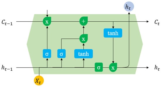
Figure 1. LSTM Structure.

Forget gate:

$$f_t=\sigma \left(W_f·\left[h_{t-1},x_t\right]+b_f\right)$$

(2)

Input gate:

$$i_t=\sigma \left(W_i·\left[h_{t-1},x_t\right]+b_i\right)$$

(3)

Candidate value:

$${\tilde{C}}_t=tanh\left(W_C·\left[h_{t-1},x_t\right]+b_C\right)$$

(4)

Cell state:

$$C_t= f_t·C_{t-1}+i_t·{\tilde{C}}_t$$

(5)

Output gate:

$$o_t=\sigma \left(W_o·\left[h_{t-1},x_t\right]+b_o\right)$$

(6)

Hidden state:

$$h_t=o_t·\tanh \left(C_t\right)$$

(7)

Table 1 provides a description of LSTM variables used. This gated mechanism allows the LSTM to effectively model both short-term and long-term dependencies in the wind speed data, which is particularly valuable for capturing recurring weather patterns, diurnal cycles, and seasonal variations inherent in the Bonavista region. Consequently, the LSTM model is well-suited for the task of short-term wind speed forecasting where temporal dynamics are crucial.

Table 1. Notation of LSTM variables.

Variable	Notation
$x_t$	Input vector at time t
$h_{t-1}$	Hidden state from previous time step
$C_{t-1}$	Cell state from previous time step
$W_f, { W}_i,{ W}_C,{ W}_o$	Weight matrices
$b_f, { b}_i, { b}_C,{ b}_o$	Bias vectors

2.4. Model Training and Evaluation Strategy

The dataset was divided chronologically into a training set covering March 2024 to February 2025 and a testing set spanning March 2025 to May 2025. This approach simulates real-world operational forecasting where future data is unavailable during training.

Model performance was evaluated using two widely accepted error metrics: Root Mean Squared Error (RMSE) and Mean Absolute Error (MAE) [19]. These are mathematically expressed as:

$$RMSE=\surd ({\displaystyle \frac{1}{n}}\sum _{i=1}^n{\left(y_i-{\widehat{y}}_i\right)}^2)$$

(8)

$$MAE={\displaystyle \frac{1}{n}}\sum _{i=1}^n{|y}_i-{\widehat{y}}_i|$$

(9)

Additionally, the Mean Absolute Percentage Error (MAPE) and Coefficient of Determination (R²) were calculated to provide a scale-independent error measure and an indication of explained variance, respectively:

$$MAPE={\displaystyle \frac{100\%}{n}}\sum _{i=1}^n\left|{\displaystyle \frac{y_i-{\widehat{y}}_i}{y_i}}\right|$$

(10)

$$R^2=1-{\displaystyle \frac{{\sum }_{i=1}^n{\left(y_i-{\widehat{y}}_i\right)}^2}{{\sum }_{i=1}^n{\left(y_i-\overline{y_i}\right)}^2}}{\displaystyle \frac{1}{n}}$$

(11)

These metrics provide intuitive interpretations of forecast accuracy in terms of the physical units of wind speed (m/s).

2.5. Model Implementation and Hyperparameters

The implementation of the LSTM model was done in TensorFlow/Keras. It includes two stacked LSTM layers (50 and 25 units, respectively), a Dropout layer (rate = 0.2) used for regularization, and a Dense output layer with linear activation function at the end. This 2-layer build was found to have an optimal trade-off between model capacity and training performance for this data set. Compilation of the model was done using an Adam optimizer with a learning rate of 0.001 and trained to limit the Mean Squared Error (MSE) loss function. The simulation used 32 batches and ran training for 10 epochs, including monitor of early stopping callback (patience = 5) to reduce validation loss and mitigate risk of overfitting. Temporally split training data into 80% for training phase and 20% validation phase.

3. Results and Analysis

The LSTM model demonstrated strong predictive performance over the three-month forecasting horizon. The RMSE and MAE values of 0.39 m/s and 0.27 m/s, respectively, indicate that the model captures the wind speed variability with reasonable precision suitable for microgrid operational decision-making. The model also achieved a MAPE of 5.73% and a R² value at 0.97, which further confirmed that it is very accurate in explaining the majority of variance in wind speed data.

3.1. Correlation Analysis

Figure 2 shows a correlation heatmap of the input variables which revealed that wind speed exhibited moderate inverse correlation with surface pressure and positive correlation with wind direction in specific ranges. This validates the inclusion of these parameters as input features.

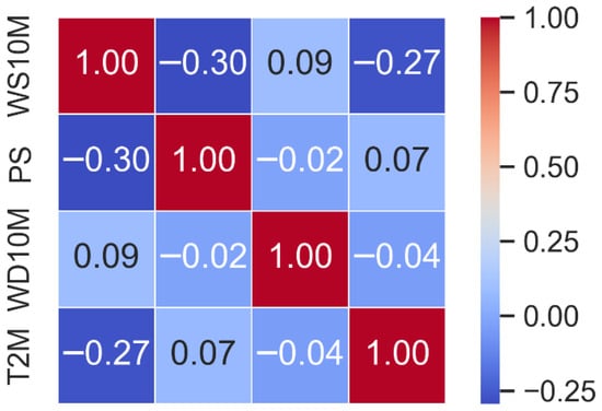
Figure 2. Correlation heatmap of attributes.

3.2. Forecast Performance

Figure 3 presents the forecast plot for March 2024 to February 2025 showing that the predicted wind speed closely follows the actual measurements.

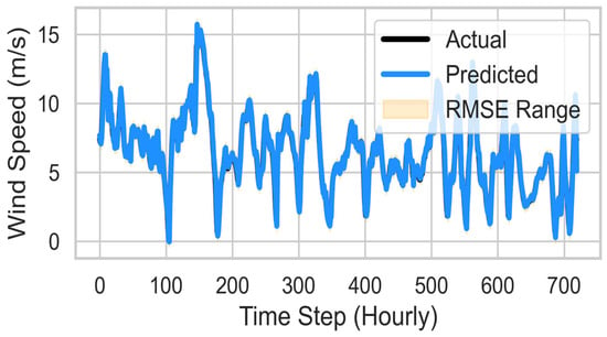
Figure 3. Forecast vs. Actual with Error Bands.

RMSE-based error bands were added to visually represent the uncertainty around the forecasts.

3.3. Error Distribution and Residuals Performance

Figure 4 illustrates an error distribution histogram which demonstrated that the errors are symmetrically distributed around zero, suggesting that the model does not systematically overestimate or underestimate wind speeds.

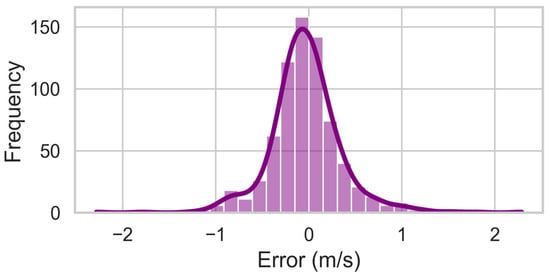
Figure 4. Histogram showing the distribution of prediction errors.

The residual plot as represented in Figure 5, which depicts errors over time, showed no significant trends or drifts, further indicating that the model generalizes well across the forecast horizon.

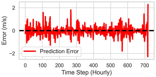
Figure 5. Residuals over time indicating error stability.

3.4. Actual vs. Predicted Scatter Plot

Figure 6 represents a scatter plot comparing actual versus predicted wind speeds displayed strong clustering around the 45-degree line, indicative of high forecast accuracy.

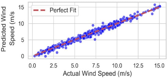
Figure 6. Actual versus predicted wind speed scatter plot.

3.5. Density Comparison

Figure 7 illustrates the Kernel density estimates of the actual and predicted wind speed distributions which showed high overlap, affirming the model’s capability to replicate the statistical characteristics of the wind speed data.

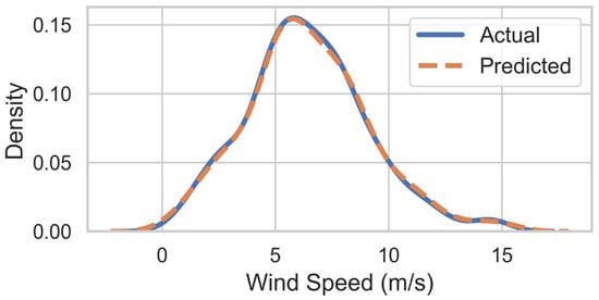
Figure 7. Comparison of probability density functions for actual and predicted wind speed.

The results confirm that the LSTM model effectively captures the temporal dependencies inherent in the wind speed data for Bonavista. The relatively low RMSE and MAE values suggest that the model is suitable for operational use in microgrid management tasks, including energy storage dispatch, demand response, and load balancing.

3.6. Model Inference Speed

The LSTM’s computational efficiency is thus critical for implementation in real-time microgrid energy management systems (EMS). The inference speed of the trained two-layer LSTM model was evaluated on a standard computing setup (Intel Core i5-8300H CPU). The average time required to generate a single one-hour-ahead wind speed prediction was approximately 8 milliseconds. This shows that the LSTM model is quite effective, and it can be easily used within real-time dispatch applications that have decision times of a few minutes to one hour, posing no computational bottleneck [20].

4. Model Comparison

4.1. Comparison to Persistence Model

The comparative analysis of the LSTM, Random Forest, and Support Vector Regression (SVR) models highlights the strengths and weaknesses of each approach in forecasting short-term wind speeds in Bonavista, NL. Compared to traditional models, LSTM’s ability to handle non-linearities and long-term dependencies gives it a significant advantage, especially for hourly forecasts over extended periods.

To further highlight the effectiveness of the proposed forecasting models, their performance was compared to a simple persistence model, which assumes that future wind speeds remain equal to the current value. This baseline is often used in wind forecasting studies due to its simplicity and surprisingly reasonable accuracy over very short horizons. Mathematically, the persistence prediction is given by:

$$\widehat{v}(t+h)=v\left(t\right)$$

(12)

where $\widehat{v}(t+h)$ is the predicted wind speed at horizon h, and $v\left(t\right)$ is the observed wind speed at the current time.

The results from Figure 8 provide useful insights of the predicting performance for each model (SVR, RF and LSTM) compared to the persistence baseline at 1, 10 and 15 h horizons. Overall, the distributions indicate that these short-term predictions pose a challenge: all three models show negative mean improvements at the 1 h horizon, indicating persistence is still very difficult to beat when the forecast window is very short [21]. However, as the time horizon is extended, the models start to benefit more clearly. For RF and LSTM, the improved positive means at both 10 and 15 h indicates that these learning-based approaches better capture broader temporal patterns which persistence accurately capture.

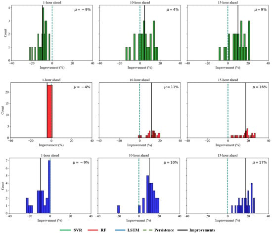
Figure 8. Distribution of forecast improvements with respect to persistence model.

Table 2 compares model performance against the persistence baseline. LSTM achieved the lowest errors, outperforming Random Forest and significantly surpassing SVR. Compared to persistence, LSTM reduced RMSE and MAE by 37% and 41%, while Random Forest achieved reductions of 27% and 30%, respectively. Additionally, LSTM also recorded the smallest MAPE of 5.73%, indicating stronger relative accuracy across varying wind speeds while maintaining a high R² value. This further demonstrates the LSTM’s ability to capture temporal and nonlinear patterns at a higher precision.

Table 2. Comparison results with baseline.

Model	RMSE (m/s)	MAE (m/s)	MAPE (%)	R2 (m/s)
LSTM	0.39	0.27	5.73	0.97
Random forest	0.45	0.32	6.73	0.97
SVR	0.997	0.79	20.87	0.86
Persistence	0.616	0.454	18.67	0.98

These findings align with prior studies [17,18,19], confirming the advantage of machine learning, especially LSTM, for longer forecasting horizons. The small gap between LSTM and Random Forest suggests both are well-suited for short-term wind forecasting in microgrid settings, whereas SVR and persistence remain less accurate.

4.2. Comparison with Related Literature

To increase the robustness of the findings and situate them in wider contemporary research, this section presents an extended comparison of the LSTM-based prediction model developed in this study with several other state-of-the-art models recently proposed in the literature. They vary from CNN-BiLSTM hybrids through attention-enhanced LSTM variants to transformer-based deep learning models.

For comparison purposes, four models were implemented and trained with the same data used in this research: the baseline LSTM, a CNN-BiLSTM as in [22], an Attention-LSTM with bidirectional architecture [23], and a lightweight Transformer model [24]. The models were compared based on RMSE, MAE, MAPE, and R² with their performances visually compared using two advanced visualization techniques: the polar wind forecast plot and the Taylor diagram.

For an unbiased analysis, all deep learning techniques (CNN-BiLSTM, Attention-LSTM, Transformer) were applied using the identical preprocessed dataset. All models were optimized using grid search to obtain key hyperparameters (number of convolutional filters, LSTM units, attention heads, learning rate) and then all trained under the same conditions to allow for a comparison.

Figure 9 presents polar scatter plots of modelled and observed wind speeds for various directions of wind from each model. These plots show the quality with which each model explains the joint magnitude–direction aspect of wind behaviour within Bonavista’s coastal environment. In all models, the great majority of time series of wind events cluster in the southwest to northwest sectors (approximately 225° to 315°), consistent with Bonavista’s coastally dominated wind patterns. The CNN-BiLSTM and LSTM models are more highly predictive of actual wind observations over the prevailing directions. They possess predicted values closely clustered around actual values, indicating that they preserve well both wind speed magnitude and directional bias.

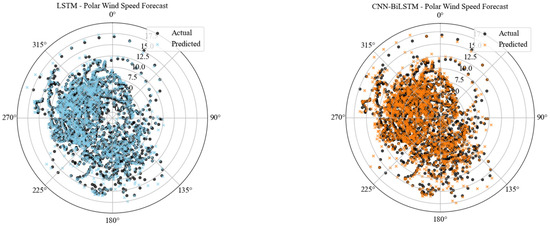
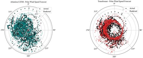
Figure 9. Polar wind forecast plot of the predictive models.

The Attention-LSTM model, while generally close agreement, possesses somewhat higher dispersal in predicted speeds between directions, particularly at 270°, indicating potential difficulties with higher-frequency directional change. On the contrary, the Transformer model has more extreme over-prediction for wind speeds, especially for events in the 180–270° range. This is evident from the spread of red predicted marks beyond the corresponding black actual values. While this model does follow the dominant directional trend, it appears to struggle more with magnitude accuracy in some regimes of winds.

Overall, the polar plots show that while all models capture dominant wind directions, the sequence-based LSTM offers greater fidelity in representing wind magnitude in this coastal setting.

Figure 10 shows the Taylor diagram which provides a compact and insightful representation of each model’s performance by simultaneously comparing the standard deviation, correlation coefficient, and centred RMSE against observed data. The plot effectively visualizes how closely each model’s output matches the reference in terms of pattern similarity and variability. Among the tested models, LSTM and CNN-BiLSTM exhibited strong correlations (r > 0.95) and standard deviations closely aligned with the reference, indicating accurate replication of wind speed dynamics. The Transformer model, while showing a lower correlation (r = 0.77), maintained a comparatively balanced standard deviation and may offer advantages in generalization under more volatile wind regimes.

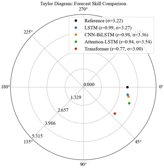
Figure 10. Taylor diagram of forecast skill for the predictive models.

A comparison of the proposed LSTM model with some recent deep learning approaches is presented in Table 3. Across the evaluated recent state-of-the-art models, LSTM achieves the lowest RMSE, MAE, and MAPE scores while still having the highest R² value. These results show that not only does the LSTM provide better forecasts, it also accounts for more variance in wind speed than CNN-BiLSTM, Attention-LSTM, and Transformer-based models.

Table 3. Model Performance Comparison Against Recent Literature.

Model	RMSE (m/s)	MAE (m/s)	MAPE (%)	R2 (m/s)
LSTM	0.39	0.27	5.73	0.97
CNN-BiLSTM [22]	0.67	0.45	8.47	0.96
Attention-LSTM [23]	1.18	0.86	20.14	0.70
Transformer [24]	2.25	1.76	36.54	0.61

5. Estimation of Wind Power Generation

While the primary focus of this study was on forecasting short-term wind speeds using machine learning models, it is also important to understand how these forecasts translate into actual wind power generation—the ultimate goal of microgrid operation planning. To this end, the predicted and actual windspeeds were converted into estimated power output using the standard wind power equation and a representative turbine model.

Wind power output at a given time can be expressed as [25]:

$$P=\left\{\begin{array}{cc}0,& v<v_{cut-in}\\ {\displaystyle \frac{1}{2}}\rho A{C}_p{v}^3,& v_{cut-in}\le v\le v_{rated}\\ P_{rated,}& v_{rated}\le v\le v_{cut-out}\end{array}\right\}$$

(13)

where:

• v is the wind speed (m/s) at time t,
• ρ is the air density,
• A is the rotor swept area,
• $C_p$ is the power coefficient, representing turbine efficiency,
• $P_{rated}$ is the rated power of the turbine,
• $v_{cut-in}, v_{rated},$ $v_{cut-out}$ are the cut-in, rated, and cut-out wind speeds, respectively.

In this study, the following assumptions were made for the turbine specifications:

• Rotor radius: 40 m;
• Rated power: 2 MW;
• Cut-in wind speed: 3 m/s;
• Rated wind speed: 12 m/s;
• Cut-out wind speed:  25 m/s.

The selected turbine parameters are representative of mid-scale turbines typically found in distributed wind projects and community microgrids in North Atlantic regions, which makes them suitable for estimating potential power generation within the context of the Bonavista microgrid [25]. Based on these assumptions, wind speeds below the cut-in or above the cut-out speeds were assigned zero power output, speeds between cut-in and rated were calculated using the cubic relation in the equation, and speeds between rated and cut-out were assigned the rated power.

The estimated power output was then computed for both actual and predicted wind speeds from all three models (LSTM, Random Forest, SVR).

Figure 11 provides a comparison plot of the estimated wind power over time. It illustrates how well the wind speed forecasts approximate the actual power output. As expected, the LSTM-based forecasts provided estimated power outputs that closely matched the actual power. In contrast, Random Forest and SVR displayed larger differences.

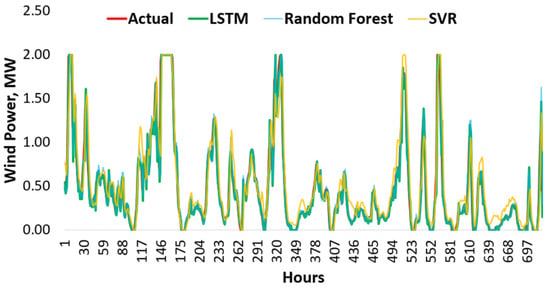
Figure 11. Estimated Wind Power Output.

It’s important to note that actual power generation can vary based on the specific wind turbine used. Different turbines have different rotor diameters, rated powers, and cut-in/cut-out speeds. The results here are based on a representative medium-sized turbine and aim to show that it’s possible to turn wind speed forecasts into useful power estimates.

Figure 12 shows the probability density distributions of forecast errors (predicted minus actual) in wind power output for the three models: Long Short-Term Memory (LSTM), Random Forest (RF), and Support Vector Regression (SVR). The horizontal axis indicates the forecast error in megawatts (MW), while the vertical axis displays the corresponding density.

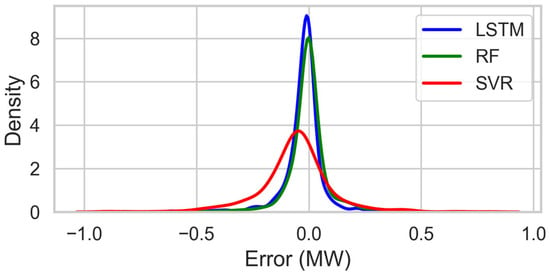
Figure 12. Probability density distributions of the forecast errors.

The LSTM model had the most focused error distribution, with a sharp peak at zero. This means that most of its predictions were very close to the actual wind power values. It suggests that LSTM not only has lower average errors, as indicated by RMSE and MAE metrics, but also maintains consistent predictions with fewer large deviations from the actual values.

The RF model also showed a tightly clustered error distribution around zero, although it was slightly wider than LSTM’s model. This indicates somewhat more variability, but overall, it still performed well. The peak density for RF was lower than that of LSTM, which corresponds to its slightly higher error metrics noted in previous analyses.

In contrast, the SVR model exhibited a broader and flatter error distribution when compared to LSTM and RF. It had a less defined peak at zero and a noticeable spread of errors in both positive and negative directions. This shows that SVR’s prediction is more scattered and less reliable, with a higher occurrence of larger errors.

Overall, the density plots clearly emphasize LSTM’s superior accuracy and reliability, closely followed by RF. Meanwhile, SVR showed the weakest performance of the three models in forecasting wind power at the microgrid level. These results support LSTM’s suitability for operational wind power forecasting, where low prediction error and stability are vital for effective microgrid management.

6. Discussion

This study presents significant insights into the use of machine learning for wind forecasting in remote coastal microgrids. The relatively simple two-layer Long Short-Term Memory (LSTM) network was superior under these conditions at generating the correct RMSE of 0.39 m/s and MAE of 0.27 m/s, which indicate that, due to the relative ease of engineering with an effective ability to recognize temporal patterns; it outperforms standard machine learning methods as well as deep learning architectures in this particular forecasting scope. This is particularly noteworthy given the growth of sophisticated neural network models in wind forecasting literature [26,27].

The architecture of the LSTM, which consists of 2 stacked recurrent layers (50 and 25), and a dense output layer, leads to an optimal balance of model size and data efficiency for the available dataset. This relatively simple architecture covered the temporal dependencies in Bonavista wind patterns and avoided the overfitting that characterizes more parameter-rich models, such as those in Transformer and Attention-LSTM variants. This architectural efficiency is further shown through the average inference speed of approximately 8 milliseconds per prediction for the model, which is suitable for deployment on the meager computing infrastructures generally accessible in remote microgrid areas.

Interpretation of the visualizations presented in this study, reveals important site-specific characteristics that inform both forecasting strategy and operational decision-making. Two polar wind plots are presented that show the most frequent southwesterly to northwesterly (225–315°) wind patterns from Bonavista’s coastal exposure to prevailing Atlantic systems. This orientation is instrumental in explaining the stability of the LSTM. Once these patterns have been learned, a predictable temporal evolution can be observed, which the LSTM networks are especially well-suited for capturing [14]. According to the Taylor chart, an improvement in both correlation and variance matching with the observed data supports the LSTM’s accuracy of prediction. The models not only predict timing correctly but capture the distribution of wind speed magnitudes from their real values.

Several limitations need to be acknowledged when interpreting these results. First, NASA POWER reanalysis data provides valuable evidence for reproducibility and accessibility. Nevertheless, there are difficulties with its resolution, which may affect forecast accuracy. The size of the data set (~35 km × 55 km in Bonavista latitude) which is about 0.5° × 0.5° does not allow microscale topographic and localized coastal breeze effects to be included that could influence the wind conditions at the turbine level [28]. Secondly, intense nor’easters common in Newfoundland were not accounted for in the dataset used for training the models. Thus, the performance of the models in extreme weather conditions is yet to be validated. Third, although the methodology exhibited strong site-specific performance, its generalizability to other locations would necessitate validation with local data. However, the efficient training methodology used in this study makes it possible to reproduce similar results.

Operationally, the forecasting system complements a number of microgrid management approaches. Converting wind speed predictions into estimated power generation enables the maximum dispatch of complementary renewables and energy sources (primarily diesel generators and battery storage systems). In the case of isolated microgrids such as Bonavista, where fuel delivery is an operational cost and logistical burden, providing reliable 3-month forecasting data helps to plan for fuel supply at the microgrid level on a quarterly basis. Additionally, the hourly forecast resolution facilitates predictive storage management that will enable operators to recharge batteries in anticipation of expected peak wind generation periods while discharging them strategically during forecast lulls.

This comparative analysis provides practical decisions for microgrid planners and operators. The two-layer LSTM model’s success indicates that the first phase of forecast implementation is better achieved through carefully optimized standard architectures before the use of more complicated solutions. This provides the balance between performance, implementation complexity and computation requirement that are crucial in resource constrained microgrid settings. Also, the high correlation between accuracy of forecast and power estimation accuracy emphasizes that reliable wind prediction is paramount for overall optimization of microgrid systems. Hybrid approaches might be considered for future implementation by combining the temporal learning of LSTMs and, where feasible, local high-resolution measurements with approaches like transfer learning or ensemble methods [20]. In addition, the results reflect the need to consider new value-oriented forecasting approaches considering feedback from microgrid optimization results. Practitioners can design predictive models integrated with the operational decisions that the predictive accuracy informs and can be used to better calibrate accuracy against actual operational benefits [29].

7. Conclusions

The application of a deep learning method for short-term wind speed forecasting in relation to microgrid operations in Bonavista, NL, was detailed in this paper. For the following three months, the LSTM model, which was trained on a year’s worth of historical data, accurately predicted wind speeds. Additionally, the model’s RMSE and MAE were lower than those of the Random Forest and SVR models. Similar results were observed when the LSTM model was compared to other deep learning methods, where it performed competitively well. Given the achieved RMSE of 0.39 m/s and an MAE of 0.27 m/s, LSTM’s computational efficiency (~8 ms inference time) and its reliable power conversion estimates make this model practically applicable for microgrid energy management.

However, there are some limitations. The reliance on NASA POWER reanalysis data, although globally available, may not capture local microscale effects, and the model’s overall robustness for severe meteorological events needs further consideration. To mitigate these limitations, additional work would consist of demonstrating the approach with higher-resolution local measurement data (for addressing the spatial limitations of this method); expanding the framework to multi-step forecasting (e.g., 6–48 h) to support better operational planning; complementing renewable sources by combining solar photovoltaic generation with other energy sources to form holistic renewable forecasting systems; employing transfer learning methods to allow for adaptation of the methodology to other remote coastal microgrids with little or no historical data; and exploring value-oriented forecasting that uses optimization decision results (for example economic dispatch or storage management) for microgrids that the forecasting method relies on, ultimately aligning forecast accuracy with operational value.

References

- Jafari, M.; Botterud, A.; Sakti, A. Decarbonizing power systems: A critical review of the role of energy storage. Renew. Sustain. Energy Rev. 2022, 158, 112077. [Google Scholar] [CrossRef]
- Ahmed, Z.; Jamil, M.; Khan, A. Short-Term Campus Load Forecasting Using CNN-Based Encoder–Decoder Network with Attention. Energies 2024, 17, 4457. [Google Scholar] [CrossRef]
- Manusov, V.Z.; Khaldarov, S.K.; Palagushkin, B.V. Short-term forecasting of wind and solar power generation. J. Phys. Conf. Ser. 2021, 2131, 052050. [Google Scholar] [CrossRef]
- Krishna, R.; S, H. Long short-term memory-based forecasting of uncertain parameters in an islanded hybrid microgrid and its energy management using improved grey wolf optimization algorithm. IET Renew. Power Gener. 2024, 18, 3640–3658. [Google Scholar] [CrossRef]
- Zhang, J.; Jiang, X.; Chen, X.; Li, X.; Guo, D.; Cui, L. Wind Power Generation Prediction Based on LSTM. In Proceedings of the 2019 4th International Conference on Mathematics and Artificial Intelligence, Chengdu, China, 12–15 April 2019; Association for Computing Machinery: New York, NY, USA, 2019; pp. 85–89. [Google Scholar]
- Giebel, A.G.; Brownsword, R.; Kariniotakis, G.; Denhard, M.; Draxl, C. The State-of-the-Art in Short-Term Prediction of Wind Power: A Literature Overview, 2nd ed.; ANEMOS.plus: Roskilde, Denmark, 2011. [Google Scholar]
- Pinson, P.; Christensen, L.E.; Madsen, H.; Sørensen, P.; Donovan, M.H.; Jensen, L.E. Regime-switching model for short-term wind power forecasting. Appl. Energy 2011, 88, 4606–4614. [Google Scholar]
- Sfetsos, A. A comparison of various forecasting techniques applied to mean hourly wind speed time series. Renew. Energy 2000, 21, 23–35. [Google Scholar] [CrossRef]
- Carta, J.; Velázquez, S.; Cabrera, P. A review of measure-correlate-predict (MCP) methods used to estimate long-term wind characteristics at a target site. Renew. Sustain. Energy Rev. 2013, 27, 362–400. [Google Scholar] [CrossRef]
- Madhukumar, M.; Sebastian, A.; Liang, X.; Jamil, M.; Shabbir, M. Regression Model-Based Short-Term Load Forecasting for University Campus Load. IEEE Access 2022, 10, 8891–8905. [Google Scholar] [CrossRef]
- Qu, K.; Xue, S.; Zheng, X.; Yan, D.; Cao, H. Learning dynamic inter-farm dependencies for wind power forecasting via adaptive sparse graph attention network. Renew. Energy 2025, 245, 124969. [Google Scholar] [CrossRef]
- Kangaji, L.M.; Raji, A.; Orumwense, E. Optimizing Sustainability Offshore Hybrid Tidal-Wind Energy Storage Systems for an Off-Grid Coastal City in South Africa. Sustainability 2024, 16, 9139. [Google Scholar] [CrossRef]
- Aguilar, D.; Quinones, J.J.; Pineda, L.R.; Ostanek, J.; Castillo, L. Optimal scheduling of renewable energy microgrids: A robust multi-objective approach with machine learning-based probabilistic forecasting. Appl. Energy 2024, 369, 123548. [Google Scholar] [CrossRef]
- Rodrigues, G.C.; Braga, R.P. Evaluation of NASA POWER Reanalysis Products to Estimate Daily Weather Variables in a Hot Summer Mediterranean Climate. Agronomy 2021, 11, 1207. [Google Scholar] [CrossRef]
- Wazirali, R.; Yaghoubi, E.; Abujazar, M.S.S.; Ahmad, R.; Vakili, A.H. State-of-the-art review on energy and load forecasting in microgrids using artificial neural networks, machine learning, and deep learning techniques. Electr. Power Syst. Res. 2023, 225, 109792. [Google Scholar] [CrossRef]
- NASA Prediction of Worldwide Energy Resource (POWER) Data Access Viewer. Available online: https://power.larc.nasa.gov/ (accessed on 25 June 2025).
- Liu, H.; Mi, X.; Li, Y. Wind speed forecasting method based on deep learning strategy using empirical wavelet transform, long short-term memory neural network and Elman neural network. Energy Convers. Manag. 2018, 156, 498–514. [Google Scholar] [CrossRef]
- de Figueiredo, Y.F.C.; de Campos, L.M.L. Wind power multi-step predictions in Northeastern Brazilian regions using artificial neural networks. In Hybrid Intelligent Systems (HIS 2020); Abraham, A., Hanne, T., Castillo, O., Gandhi, N., Rios, T.N., Hong, T.-P., Eds.; Advances in Intelligent Systems and Computing; Springer: Cham, Switzerland, 2021; Volume 1375, pp. 649–658. [Google Scholar] [CrossRef]
- de Araujo, J.S. Combination of WRF model and LSTM network for solar radiation forecasting-Timor Leste case study. Comput. Water Energy Environ. Eng. 2020, 9, 108–144. [Google Scholar] [CrossRef]
- Chen, Z.; Blair, H.; Cong, J. Energy Efficient LSTM Inference Accelerator for Real-Time Causal Prediction. ACM Trans. Des. Autom. Electron. Syst. 2022, 27, 1–19. [Google Scholar] [CrossRef]
- Dantas, G.; Browell, J. Seamless short- to mid-term probabilistic wind power forecasting. arXiv 2025, arXiv:2502.11960. [Google Scholar] [CrossRef]
- Hossain, M.A.; Chakrabortty, R.K.; Elsawah, S.; Ryan, M.J. Very short-term forecasting of wind power generation using hybrid deep learning model. J. Clean. Prod. 2021, 296, 126564. [Google Scholar] [CrossRef]
- de Aquino, R.R.B.; Ludermir, T.B.; Neto, O.N.; Ferreira, A.A.; Lira, M.M.S.; Carvalho, M.A. Forecasting models of wind power in Northeastern of Brazil. In Proceedings of the 2013 International Joint Conference on Neural Networks (IJCNN), Dallas, TX, USA, 4–9 August 2013; pp. 1–8. [Google Scholar] [CrossRef]
- Ahmed, Z.; Jamil, M.; Khan, A. A Novel Multi-Task Learning-Based Approach to Multi-Energy System Load Forecasting. IEEE Open Access J. Power Energy 2025, 12, 209–219. [Google Scholar]
- Ibrahim, A.; Mirjalili, S.; El-Said, M.; Ghoneim, S.S.M.; Al-Harthi, M.M.; Ibrahim, T.F.; El-Kenawy, E.M. Wind speed ensemble forecasting based on deep learning using adaptive dynamic optimization algorithm. IEEE Access 2021, 9, 125456–125471. [Google Scholar] [CrossRef]
- Zhu, M.; Li, Z.; Lin, Q.; Ding, L. Fast-Powerformer: A memory-efficient transformer for accurate mid-term wind power forecasting. arXiv 2025, arXiv:2504.10923. [Google Scholar] [CrossRef]
- Liao, W.; Bak-Jensen, B.; Pillai, J.R.; Yang, Z.; Liu, K. Short-term power prediction for renewable energy using hybrid graph convolutional network and long short-term memory approach. arXiv 2021, arXiv:2111.07958. [Google Scholar] [CrossRef]
- Rosa, S.; Souza, J.; Santos, A. Data from NASA Power and surface weather stations under different climates on reference evapotranspiration estimation. Pesqui. Agropecuária Bras. 2023, 58, e03261. [Google Scholar] [CrossRef]
- Zhang, Y.; Jia, M.; Wen, H.; Bian, Y.; Shi, Y. Toward Value-Oriented Renewable Energy Forecasting: An Iterative Learning Approach. IEEE Trans. Smart Grid 2024, 15, 350–364. [Google Scholar] [CrossRef]
Disclaimer/Publisher’s Note: The statements, opinions and data contained in all publications are solely those of the individual author(s) and contributor(s) and not of MDPI and/or the editor(s). MDPI and/or the editor(s) disclaim responsibility for any injury to people or property resulting from any ideas, methods, instructions or products referred to in the content. |
© 2026 by the authors. Licensee MDPI, Basel, Switzerland. This article is an open access article distributed under the terms and conditions of the Creative Commons Attribution (CC BY) license.