A Method for Asymmetric Fault Location in HVAC Transmission Lines Based on the Modal Amplitude Ratio

Abstract

To address the issues of insensitivity to high-impedance ground faults and difficulty in identifying reflected wavefronts in single-ended traveling-wave fault location methods for asymmetric ground faults in high-voltage AC transmission lines, this paper proposes a single-ended fault location method based on the modal amplitude ratio and deep learning. First, based on the dispersion characteristics of traveling waves, an approximate formula is derived between the fault distance and the amplitude ratio of the sum of the initial transient voltage traveling-wave 1-mode and 2-mode to 0-mode at the measurement point. Simulation verifies that the fault distance x from the measurement point at the line head is unaffected by transition resistance and fault inception angle, and that a nonlinear positive correlation exists between the distance x and the modal amplitude ratio. The multi-scale wavelet modal maximum ratio of the sum of 1-mode and 2-mode to 0-mode is used to characterize the amplitude ratio. This ratio serves as the input for a Residual Bidirectional Long Short-Term Memory (BiLSTM) network, which is optimized using the Dung Beetle Optimizer (DBO). The DBO-Res-BiLSTM model fits the nonlinear mapping between the fault distance x and the amplitude ratio. Simulation results demonstrate that the proposed method achieves high location accuracy. Furthermore, it remains robust against variations in fault type, location, transition resistance, and inception angle.

1. Introduction

High-voltage alternating current (HVAC) transmission lines play a crucial role in power transmission, responsible for delivering electrical energy from generation sources to load centers. In actual operation, asymmetric ground faults are the most common type of fault in HVAC lines, with single-phase ground faults accounting for over 80% of total faults [1]. After a fault occurs, rapid and accurate fault location is essential not only for timely line repair and power restoration but also for the economical, secure, and stable operation of the power system [2].

Traditional fault location methods mainly include impedance-based methods and traveling-wave methods. Impedance-based methods are now seldom used due to their relatively large errors. Traveling-wave methods can be divided into single-ended and double-ended approaches. Reference [3] proposed a single-ended traveling-wave location method combining wavefront steepness and wavelet-based wavefront identification; reference [4] introduced a novel single-ended fault location method for hybrid parallel HVAC/HVDC lines sharing the same tower. However, single-ended methods struggle to effectively identify reflected wavefronts. Reference [5] proposed a double-ended location method combining inherent frequency-based rough location and wavefront calibration using Ensemble Empirical Mode Decomposition (EEMD); reference [6] presented a fault detection and location technique for multi-terminal DC microgrids based on local measurement data. Nevertheless, double-ended methods require additional measurement devices and synchronization equipment, and their accuracy is affected by data asynchrony between the two ends. Traveling-wave location methods typically employ distributed parameter models [7,8,9,10,11]; however, studies have shown that the wave velocity calculated based on distributed parameters deviates from the actual velocity [12,13,14,15]. Reference [13] proposed an improved single-ended traveling-wave method that detects signal arrival times and wave polarity, which can address reflected wave identification but still introduces errors due to approximate wave velocity estimation.

In recent years, with the synergistic development of artificial intelligence and the power industry, intelligent algorithms based on machine learning have achieved significant results in HVAC transmission line fault location. The excellent nonlinear fitting capability of machine learning enables it to handle tasks that are difficult for impedance-based, traveling-wave, and inherent frequency methods [16]. Reference [17] developed an intelligent location system based on multiple random forest technology for single-phase ground fault location in wind farms, though its effectiveness on HVAC lines remains to be verified. Reference [18] employed a maximum mean discrepancy algorithm to classify different transmission lines and adopted a double-ended CNN-LSTM combined model for fault location. This method does not rely on line parameters or models but requires synchronized data from both ends, making it relatively complex for practical applications.

Traditional traveling-wave location methods still face challenges in wavefront identification, arrival time calibration, and wave velocity estimation [19]. To overcome these difficulties, this paper proposes a single-ended fault location method based on the modal amplitude ratio and deep learning for asymmetric ground faults in HVAC lines. It is noteworthy that the method proposed in this study primarily targets the most common asymmetric ground faults in HVAC transmission lines, such as single-phase-to-ground and double-phase-to-ground faults. These faults generate a distinct zero-sequence mode component, and the proposed mode amplitude ratio method is fundamentally based on the analysis of this component. Consequently, the method is not directly applicable to fault types that do not produce a zero-mode component, such as phase-to-phase faults. Delimiting the scope to ground faults allows for a focused investigation and enables the development of a more precise and robust solution for this predominant scenario. A detailed discussion on the scope of applicability is provided in Section 2.2.

Compared to existing methods, the main novelty and contributions of this work are threefold:

(1)

Conceptual innovation. Unlike traditional traveling-wave methods that strive to suppress or compensate for errors induced by dispersion [20,21], this paper is the first to proactively utilize the variation pattern of modal amplitudes caused by traveling-wave dispersion, transforming it into a direct representation of fault distance, thereby offering a new physical perspective for fault location.

(2)

Methodological innovation. A single-ended location principle based on the mode amplitude ratio is proposed, coupled with the construction of a “DBO-Res-BiLSTM” intelligent mapping model. This method requires only the detection of the initial voltage traveling-wavefront, eliminating the need for reflected wave identification, precise arrival time calibration, or wave velocity calculation, thus fundamentally avoiding the primary error sources of conventional single-ended methods.

(3)

Performance improvement. The proposed method has inherent robustness to transition resistance and fault initiation angle. The simulation results show that its positioning accuracy is significantly better than traditional A-type traveling wave method and other deep learning models, providing an effective solution for the precise positioning of high impedance grounding faults.

In summary, this work not only introduces a novel fault location philosophy but also delivers a practical, robust, and highly accurate solution for ground fault location in HVAC transmission systems.

2. Fault Location Principle for Asymmetric Grounding Faults

The three-phase voltage at the head end of the HVAC transmission line before the fault can be expressed as follows:

$$\left\{\begin{array}{l}{u}_A(t)=\sqrt{2}U\cos (\omega t)\\ u_B(t)=\sqrt{2}U\cos (\omega t-120°)\\ u_C(t)=\sqrt{2}U\cos (\omega t+120°)\end{array}\right.$$

(1)

Under normal operating conditions, the relationship between the voltage at a point located a distance x from the line head end before the fault and the voltage at the head end is given by the following [19]:

$$\left\{\begin{array}{l}{u}_{Ax}=u_A(t)e^{-{\displaystyle \frac{r_0}{2z}}x}=\sqrt{2}U\cos (\omega t)e^{-{\displaystyle \frac{r_0}{2z}}x}\\ u_{Bx}=u_B(t)e^{-{\displaystyle \frac{r_0}{2z}}x}=\sqrt{2}U\cos (\omega t-{120}^{\circ })e^{-{\displaystyle \frac{r_0}{2z}}x}\\ u_{Cx}=u_C(t)e^{-{\displaystyle \frac{r_0}{2z}}x}=\sqrt{2}U\cos (\omega t+{120}^{\circ })e^{-{\displaystyle \frac{r_0}{2z}}x}\end{array}\right.$$

(2)

where $u_{Ax}(t)$ is the phase A voltage at the point distance x from the sending end; $u_{Bx}(t)$ is the phase B voltage at that point; $u_{Cx}(t)$ is the phase C voltage at that point; r₀ is the resistance per unit length of the conductor; z is the surge impedance of the line.

Asymmetric ground faults include single-phase-to-ground faults and two-phase-to-ground faults. When a ground fault occurs at point f on a HVAC transmission line, according to the superposition theorem, the transient traveling-wave process is equivalent to the sudden superimposition of a voltage at the fault point that is equal in magnitude but opposite in direction to the pre-fault voltage.

2.1. Location Principle for Single-Line-to-Ground Faults

Taking an A-phase-to-ground fault as an example, and considering the influence of the transition resistance R_f, the initial transient voltage traveling waves for each mode at the fault point can be derived from reference [20]:

$$\left\{\begin{array}{l}\begin{array}{c}{u}_{f0}^{(1)}=-{\displaystyle \frac{Z_0}{Z_0+Z_1+Z_2+6R_f}}{u}_{\mathrm{Ax}}(t)=-{\displaystyle \frac{Z_0\sqrt{2}U\cos (\omega t){\mathrm{e}}^{-\frac{r_0}{2z^x}}}{Z_0+Z_1+Z_2+6R_f}}\\ u_{f1}^{(1)}=-{\displaystyle \frac{Z_1}{Z_0+Z_1+Z_2+6R_f}}{u}_{\mathrm{A}x}(t)=-{\displaystyle \frac{Z_1\sqrt{2}U\cos (\omega t){\mathrm{e}}^{-\frac{r_0}{2z^x}}}{Z_0+Z_1+Z_2+6R_f}}\end{array}\\ u_{f2}^{(1)}=-{\displaystyle \frac{Z_2}{Z_0+Z_1+Z_2+6R_f}}{u}_{\mathrm{Ax}}(t)=-{\displaystyle \frac{Z_2\sqrt{2}U\cos (\omega t){\mathrm{e}}^{-\frac{r_0}{2z^x}}}{Z_0+Z_1+Z_2+6R_f}}\end{array}\right.$$

(3)

where $u_{f0}^{(1)}$, $u_{f1}^{(1)}$ and $u_{f2}^{(1)}$ are the initial transient voltage traveling-wave components for mode 0, mode 1, and mode 2, respectively, for an A-phase-to-ground fault at the fault point; $Z_0$, $Z_1$ and $Z_2$ are the surge impedances for mode 0, mode 1, and mode 2 of the HVAC transmission line, respectively.

The line j th (j = 0, 1, 2) modal propagation coefficient ${\gamma }_j$ and the propagation function $A_j$ for a HVAC transmission line of length x can be defined as follows:

$$A_j(\mathrm{j}\omega )={\displaystyle \frac{u_j(\mathrm{j}\omega )}{u_f(\mathrm{j}\omega )}}={\mathrm{e}}^{-{\gamma }_{j}x}$$

(4)

$${\gamma }_j=\sqrt{(R_j+\mathrm{j}\omega L_j)\times \mathrm{j}\omega K_j}={\alpha }_j+j{\beta }_j$$

(5)

where $j=0$, $j=1$, $j=2$ are 0 mode, 1 mode, 2 mode, respectively, $\omega$ is the angular frequency of the system, $u_j(\mathrm{j}\omega )$, $u_f(\mathrm{j}\omega )$ is the modal voltage at the ranging place and the fault point, respectively, $R_j$, $L_j$, $K_j$ are the modal resistance, inductance and capacitance per unit length of the line, respectively, ${\alpha }_j$ is the modal attenuation constant of the line, ${\beta }_j$ is the modal phase coefficient of the line.

For a uniformly transposed three-phase line, the parameters of the 1-mode and 2-mode components are identical. In practical engineering scenarios involving non-uniformly transposed lines, although geometric asymmetry introduces slight discrepancies between these two aerial modes, their propagation characteristics remain highly similar. Unlike the 0-mode, which is significantly affected by the ground return path leading to substantial parameter variations, the 1-mode and 2-mode are primarily determined by the inter-conductor geometry and air insulation. Consequently, the differences in impedance and attenuation between them are negligible compared to the 0-mode. Therefore, within the allowable error margin for fault location engineering, it is reasonable to approximate ${\gamma }_1={\gamma }_2$. From Equation (4), the relationship between the initial transient voltage traveling wave modal at the line terminal and that at the fault point for a single-line-to-ground fault can be derived as follows:

$$u_0^{(1)}\left(\mathrm{j}\omega \right)={\mathrm{e}}^{-{\gamma }_{0}x}{u}_{f0}^{(1)}\left(\mathrm{j}\omega \right)=-{\displaystyle \frac{Z_0}{Z_0+Z_1+Z_2+6R_f}}{u}_{Ax}(t){\mathrm{e}}^{-{\gamma }_{0}x}=-{\displaystyle \frac{Z_0\sqrt{2}U\cos (\omega t)}{Z_0+Z_1+Z_2+6R_f}}{\mathrm{e}}^{-{\gamma }_{0}x}{\mathrm{e}}^{-{\displaystyle \frac{r_0}{2z^x}}}$$

(6)

$$u_1^{(1)}\left(\mathrm{j}\omega \right)={\mathrm{e}}^{-{\gamma }_{1}x}{u}_{f1}^{(1)}\left(\mathrm{j}\omega \right)=-{\displaystyle \frac{Z_1}{Z_0+Z_1+Z_2+6R_f}}{u}_{Ax}(t){\mathrm{e}}^{-{\gamma }_{1}x}=-{\displaystyle \frac{Z_1\sqrt{2}U\cos (\omega t)}{Z_0+Z_1+Z_2+6R_f}}{\mathrm{e}}^{-{\gamma }_{1}x}{\mathrm{e}}^{-{\displaystyle \frac{r_0}{2z^x}}}$$

(7)

$$u_2^{(1)}\left(\begin{array}{c}\mathrm{j}\omega \end{array}\right)={\mathrm{e}}^{-{\gamma }_{2}x}{u}_{f2}^{(1)}\left(\begin{array}{c}\mathrm{j}\omega \end{array}\right)=-{\displaystyle \frac{Z_2}{Z_0+Z_1+Z_2+6R_f}}{u}_{Ax}(t){\mathrm{e}}^{-{\gamma }_{2}x}=-{\displaystyle \frac{Z_2\sqrt{2}U\cos (\omega t)}{Z_0+Z_1+Z_2+6R_f}}{\mathrm{e}}^{-{\gamma }_{2}x}{\mathrm{e}}^{-{\displaystyle \frac{r_0}{2z^x}}}$$

(8)

where $u_0^{\left(1\right)}\left(j\omega \right)$, $u_1^{\left(1\right)}\left(j\omega \right)$, $u_2^{\left(1\right)}\left(j\omega \right)$ are the 0-mode, 1-mode, and 2-mode voltages at the measurement point, respectively; ${\gamma }_0$, ${\gamma }_1$, ${\gamma }_2$ are the propagation coefficients for the 0-mode, 1-mode, and 2-mode voltage traveling waves, respectively.

From Equations (6)–(8), we obtain the following:

$${\displaystyle \frac{u_1^{(1)}\left(\mathrm{j}\omega \right)+u_2^{(1)}\left(\mathrm{j}\omega \right)}{u_0^{(1)}\left(\mathrm{j}\omega \right)}}={\displaystyle \frac{u_{\mathrm{A}x}\left(t\right)\left({\mathrm{e}}^{-{\gamma }_{1}x}{Z}_1+{\mathrm{e}}^{-{\gamma }_{2}x}{Z}_2\right)}{u_{\mathrm{A}x}\left(t\right){\mathrm{e}}^{-{\gamma }_{0}x}{Z}_0}}={\displaystyle \frac{(Z_1+Z_2)}{Z_0}}{\mathrm{e}}^{({\gamma }_0-{\gamma }_1)x}$$

(9)

Taking the magnitude on both sides of Equation (9) yields the following:

$$\left|{\displaystyle \frac{u_1^{(1)}\left(\mathrm{j}\omega \right)+u_2^{(1)}\left(\mathrm{j}\omega \right)}{u_0^{(1)}\left(\mathrm{j}\omega \right)}}\right|=\left|{\displaystyle \frac{Z_1+Z_2}{Z_0}}\right|{\mathrm{e}}^{({\alpha }_0-{\alpha }_1)x}$$

(10)

Let $\left|(Z_1+Z_2)/Z_0\right|=1/k_1$ and $u_{12}^{\left(1\right)}\left(j\omega \right)=u_1^{\left(1\right)}\left(j\omega \right)+u_2^{\left(1\right)}\left(j\omega \right)$. When the structure and parameters of the HVAC transmission line are fixed, Z₀, Z₁, Z₂, α₀, α₁ are constants, resulting in the following:

$$x={\displaystyle \frac{1}{{\alpha }_0-{\alpha }_1}}\ln \left(k_1{\displaystyle \frac{\mid u_{12}^{(1)}\left(\mathrm{j}\omega \right)\mid }{\mid u_0^{(1)}\left(\mathrm{j}\omega \right)\mid }}\right)$$

(11)

Equation (11) indicates that for a single-line-to-ground fault, the fault distance x is related to the amplitude ratio of the sum of the 1-mode and 2-mode components to the 0-mode component of the initial transient voltage traveling wave at the measurement point. When a high-resistance single-line-to-ground fault occurs on the HVAC line, the fault resistance R_f affects the amplitudes of the 1-mode, 2-mode, and 0-mode components of the fault point voltage. According to Equation (9), the amplitude ratio of the sum of the 1-mode and 2-mode voltages to the 0-mode voltage at the measurement point is independent of R_f, thus eliminating the influence of fault resistance. The fault inception angle affects the amplitudes of the 1-mode, 2-mode, and 0-mode components of the fault point voltage. Similarly, Equation (9) shows that when calculating this amplitude ratio at the measurement point, the initial transient voltage wavefront amplitude $u_{Ax}(t)$ is eliminated, meaning the amplitude ratio is also independent of the fault inception angle. Therefore, for a single-line-to-ground fault, the amplitude ratio of the sum of the initial transient 1-mode and 2-mode voltages to the 0-mode voltage at the measurement point is unaffected by both the fault resistance and the fault inception angle.

2.2. Location Principle for Double-Line-to-Ground Faults

Taking a phase-B-and-C-to-ground fault as an example and considering the influence of the fault resistance R_f, the initial transient voltage traveling wave modal components at the fault point can be similarly derived as follows:

$$\left\{\begin{array}{l}{u}_{f0}^{\left(1,1\right)}={\displaystyle \frac{Z_0}{Z_m}}{u}_{Ax}\left(t\right)={\displaystyle \frac{Z_0}{Z_m}}\sqrt{2}U\cos \left(\omega t\right)e^{-{\displaystyle \frac{r_0}{2z^x}}}\\ u_{f1}^{\left(1,1\right)}={\displaystyle \frac{Z_0+2Z_1}{3Z_1\times Z_m}}{u}_{Bx}\left(t\right)+{\displaystyle \frac{Z_1-Z_0}{3Z_1\times Z_m}}{u}_{Cx}\left(t\right)={\displaystyle \frac{Z_0+2Z_1}{3Z_1\times Z_m}}\sqrt{2}U\cos \left(\omega t-{120}^{°}\right)e^{-{\displaystyle \frac{r_0}{2z^x}}}+\\ {\displaystyle \hspace{1em}\hspace{1em} \frac{Z_1-Z_0}{3Z_1\times Z_m}}\sqrt{2}U\cos \left(\omega t+{120}^{°}\right)e^{-{\displaystyle \frac{r_0}{2z^x}}}\\ u_{f2}^{\left(1,1\right)}={\displaystyle \frac{Z_1-Z_0}{3Z_1\times Z_m}}{u}_{Bx}\left(t\right)+{\displaystyle \frac{Z_0+2Z_1}{3Z_1\times Z_m}}{u}_{Cx}\left(t\right)={\displaystyle \frac{Z_1-Z_0}{3Z_1\times Z_m}}\sqrt{2}U\cos \left(\omega t-{120}^{°}\right)e^{-{\displaystyle \frac{r_0}{2z^x}}}+\\ {\displaystyle \hspace{1em}\hspace{1em} \frac{Z_0+2Z_1}{3Z_1\times Z_m}}\sqrt{2}U\cos \left(\omega t+{120}^{°}\right)e^{-{\displaystyle \frac{r_0}{2z^x}}}\end{array}\right.$$

(12)

where $Z_m=2Z_0+Z_1+12R_f$; $u_{f0}^{\left(1,1\right)}$, $u_{f1}^{\left(1,1\right)}$, $u_{f2}^{\left(1,1\right)}$ are the 0-mode, 1-mode, and 2-mode components, respectively, of the initial transient voltage traveling wave for a phase-B-and-C-to-ground fault at the fault point.

From Equation (4), the relationship between the initial transient voltage traveling wave modal components at the sending-end measurement point and those at the fault point for a double-line-to-ground fault can be derived as follows:

$$u_0^{(1,1)}\left(\begin{array}{c}\mathrm{j}\omega \end{array}\right)={\mathrm{e}}^{-{\gamma }_{0}x}{u}_{f0}^{(1,1)}\left(\begin{array}{c}\mathrm{j}\omega \end{array}\right){=\mathrm{e}}^{-{\gamma }_{0}x}{\displaystyle \frac{Z_0}{Z_{\mathrm{m}}}}{u}_{\mathrm{A}x}(t)={\displaystyle \frac{Z_0}{Z_{\mathrm{m}}}}\sqrt{2}U\cos (\omega t){\mathrm{e}}^{-{\gamma }_{0}x}{\mathrm{e}}^{-{\displaystyle \frac{r_0}{2z^x}}}$$

(13)

$$\begin{array}{c}{u}_1^{(1,1)}\left(\mathrm{j}\omega \right)={\mathrm{e}}^{-{\gamma }_{1}x}{u}_{f1}^{(1,1)}\left(\mathrm{j}\omega \right)=\left({\displaystyle \frac{Z_0+2Z_1}{3Z_1\times Z_m}}{u}_{Bx}(t)+{\displaystyle \frac{Z_1-Z_0}{3Z_1\times Z_m}}{u}_{Cx}(t)\right){\mathrm{e}}^{-{\gamma }_{1}x}{\mathrm{e}}^{-{\displaystyle \frac{r_0}{2z^x}}}\\ \hspace{1em}\hspace{1em}\hspace{1em}\hspace{1em}\hspace{1em}\hspace{1em}\hspace{1em}\hspace{1em} =\left({\displaystyle \frac{Z_0+2Z_1}{3Z_1\times Z_m}}\sqrt{2}U\cos (\omega t-{120}^{\circ })+\right.\left.{\displaystyle \frac{Z_1-Z_0}{3Z_1\times Z_{\mathrm{m}}}}\sqrt{2}U\cos (\omega t+{120}^{\circ })\right){\mathrm{e}}^{-{\gamma }_{1}x}{\mathrm{e}}^{-{\displaystyle \frac{r_0}{2z^x}}}\end{array}$$

(14)

$$\begin{array}{c}{u}_2^{(1,1)}\left(\mathrm{j}\omega \right)={\mathrm{e}}^{-{\gamma }_{2}x}{u}_{f2}^{(1,1)}\left(\mathrm{j}\omega \right)={\mathrm{e}}^{-{\gamma }_{1}x}{u}_{f2}^{(1,1)}\left(\mathrm{j}\omega \right)=\left({\displaystyle \frac{Z_1-Z_0}{3Z_1\times Z_m}}{u}_{Bx}(t)+{\displaystyle \frac{Z_0+2Z_1}{3Z_1\times Z_m}}{u}_{Cx}(t)\right){\mathrm{e}}^{-{\gamma }_{1}x}{\mathrm{e}}^{-{\displaystyle \frac{r_0}{2z^x}}}\\ \hspace{1em} =\left({\displaystyle \frac{Z_1-Z_0}{3Z_1\times Z_m}}\sqrt{2}U\cos (\omega t-{120}^{\circ })+\left.{\displaystyle \frac{Z_0+2Z_1}{3Z_1\times Z_m}}\sqrt{2}U\cos (\omega t+{120}^{\circ })\right)\right.{\mathrm{e}}^{-{\gamma }_{1}x}{\mathrm{e}}^{-{\displaystyle \frac{r_0}{2z^x}}}\end{array}$$

(15)

From Equations (13)–(15), we obtain:

$$\begin{array}{c}{\displaystyle \frac{u_1^{(1,1)}\left(\mathrm{j}\omega \right)+u_2^{(1,1)}\left(\mathrm{j}\omega \right)}{u_0^{(1,1)}\left(\mathrm{j}\omega \right)}}={\displaystyle \frac{\left(\frac{3Z_1}{3Z_1\times Z_m}{u}_{Bx}(t)+\frac{3Z_1}{3Z_1\times Z_m}{u}_{Cx}(t)\right){\mathrm{e}}^{-{\gamma }_{1}x}}{\frac{Z_0}{Z_m}{u}_{Ax}(t){\mathrm{e}}^{-{\gamma }_{0}x}}}\\ \hspace{1em}\hspace{1em}\hspace{1em}\hspace{1em}\hspace{1em}\hspace{1em}\hspace{1em}\hspace{1em}\hspace{1em}\hspace{1em}\hspace{1em}\hspace{1em}\hspace{1em}\hspace{1em}\hspace{1em}\hspace{1em}\hspace{1em}\hspace{1em} ={\displaystyle \frac{\cos (\omega t-{120}^{\circ })+\cos (\omega t+{120}^{\circ })}{Z_0\cos (\omega t)}}{\mathrm{e}}^{({\gamma }_0-{\gamma }_1)x}=-{\displaystyle \frac{1}{Z_0}}{\mathrm{e}}^{({\gamma }_0-{\gamma }_1)x}\end{array}$$

(16)

Taking the amplitude on both sides of Equation (16) yields the following:

$$\left|{\displaystyle \frac{u_1^{(1,1)}\left(\mathrm{j}\omega \right)+u_2^{(1,1)}\left(\mathrm{j}\omega \right)}{u_0^{(1,1)}\left(\mathrm{j}\omega \right)}}\right|=\left|{\displaystyle \frac{1}{Z_0}}\right|{\mathrm{e}}^{({\alpha }_0-{\alpha }_1)x}$$

(17)

Let $\left|1/Z_0\right|=1/k_2$ and $u_{12}^{(1,1)}\left(\mathrm{j}\omega \right)=u_1^{(1,1)}\left(\mathrm{j}\omega \right)+u_2^{(1,1)}\left(\mathrm{j}\omega \right)$ When the structure and parameters of the HVAC transmission line are fixed, Z₀, α₀, α₁ are constants, resulting in the following:

$$x={\displaystyle \frac{1}{{\alpha }_0-{\alpha }_1}}\ln \left(k_2{\displaystyle \frac{|u_{12}^{(1,1)}(\mathrm{j}\omega )|}{|u_0^{(1,1)}(\mathrm{j}\omega )|}}\right)$$

(18)

Equation (18) indicates that for a double-line-to-ground fault, the fault distance x is related to the amplitude ratio of the sum of the 1-mode and 2-mode components to the 0-mode component of the initial transient voltage traveling wave at the measurement point. When a high-resistance double-line-to-ground fault occurs, the fault resistance R_f affects the amplitudes of the modal components. According to Equation (16), the amplitude ratio at the measurement point is independent of R_f, eliminating its influence. The fault inception angle affects the amplitudes, but similarly, Equation (16) shows that the initial transient voltage wavefront amplitudes $u_{Ax}(t)$, $u_{Bx}(t)$, $u_{Cx}(t)$ are eliminated during the ratio calculation, making the amplitude ratio independent of the fault inception angle. Therefore, for a double-line-to-ground fault, this amplitude ratio is also unaffected by fault resistance and inception angle.

Consequently, by summarizing and deriving from Equations (11) and (18), the fault location formula for asymmetric grounding faults on HVAC transmission lines can be expressed as follows:

$$x={\displaystyle \frac{1}{{\alpha }_0-{\alpha }_1}}\ln \left(k_{\mathrm{n}}{\displaystyle \frac{\mid u_{12}(\mathrm{j}\omega )\mid }{\mid u_0(\mathrm{j}\omega )\mid }}\right)$$

(19)

where $u_{12}\left(j\omega \right)$ and $u_0\left(j\omega \right)$ are the sum of the 1-mode and 2-mode components, and the 0-mode component, respectively, of the initial transient voltage at the measurement point; $k_n$ is a constant related to the specific type of asymmetric grounding fault.

It is important to note that the zero-mode component exists only for ground faults, not for phase-to-phase faults. Therefore, Equation (19) becomes invalid for non-ground faults. However, asymmetric grounding faults are the most common type of fault on HVAC transmission lines. Phase-to-phase faults, open-circuit faults, and lightning strike faults occur with very low probability and often have more detectable characteristics. Thus, using Equation (19), it is possible to locate the prevalent and less easily discernible asymmetric grounding faults. Moreover, since it is unaffected by fault inception angle and transition resistance, this approach essentially meets the requirements for fault location of asymmetric grounding faults on HVAC transmission lines.

2.3. Neural Network-Based Fault Location Algorithm Using Wavelet Modal Maxima Ratio of Initial Traveling Waves

2.3.1. Wavelet Selection and Modal Maxima Extraction

Transient signals in power systems are typical non-stationary signals. Currently, it is not easy to extract the amplitude of a single-frequency transient signal, and time-domain analysis methods also cannot accurately obtain the amplitude of each frequency component in transient non-stationary signals. Therefore, the wavelet decomposition method is adopted to characterize the fault features at a specific frequency point using the frequency band signal near that point, overcoming the difficulty of extracting single-frequency signals.

According to the frequency-dependent characteristic of HVAC transmission lines, the surge impedance of the sum of voltage 1-mode, 2-mode and 0-mode components is relatively stable in the high-frequency range. Hence, the high-frequency transient voltage traveling wave is selected for analysis. With a sampling frequency of 1 MHz and a time-window length of 5 ms, wavelet decomposition tests were performed for three different wavelets for an asymmetric ground fault occurring at a point 50 km from the measurement device, as shown in Table 1.

Table 1. Effect of Different Waves on the Ratio of Maximum Amplitude of Wave Modes at a Distance of 5 km.

Fault Type	Single-Phase Ground Fault
Employing Wavelets	0 Ω Grounding	100 Ω Grounding	200 Ω Grounding
Haar	1.736560	1.725224	1.706325
Db4	1.716523	1.715191	1.713695
Bior3.3	1.776276	1.776915	1.776382
Fault Type	Double-Phase Ground Fault
Employing Wavelets	0 Ω Grounding	100 Ω Grounding	200 Ω Grounding
Haar	0.842887	0.831704	0.813059
Db4	0.860003	0.859027	0.857949
Bior3.3	0.888617	0.888138	0.888085

As can be seen from Table 1, the Bior3.3 wavelet delivers the highest decomposition accuracy. Therefore, this paper employs the Bior3.3 wavelet for wavelet decomposition, and the wavelet scale d1 is selected.

2.3.2. DBO-Res-BiLSTM Location Algorithm

In practical engineering, when asymmetric faults occur in HVAC transmission lines, the surge impedance and attenuation coefficient are difficult to calculate and are influenced by the line structure and specific parameters. Machine learning, with its excellent nonlinear learning capability, can bypass these complex parameter calculations and make fault location easier to implement. Residual Bidirectional Long Short-Term Memory (Res-BiLSTM) is an improved model that combines residual connections and a bidirectional long short-term memory network. Through the synergistic effect of both, it significantly enhances sequence modeling capability. The skip connections within the residual blocks effectively alleviate the depth limitation and gradient issues of BiLSTM, while ensuring sufficient capture of contextual information, thereby markedly strengthening the model’s nonlinear expressive ability.

The core concept of residual networks is that each additional layer should more readily incorporate the original function as one of its elements. Let the original input be x, and the ideal mapping to be learned be f(x) [22], as shown in Equation (20).

$$y=f(x,(W_i))+f(x)$$

(20)

In practice, residual mapping tends to be more tractable and is better suited for capturing subtle variations in the identity function. The input can propagate rapidly forward through cross-layer data pathways.

The LSTM network is a type of Recurrent Neural Network (RNN). Its advantage lies in its ability to integrate the current state of the model to produce an output for the input at each time step.

Two independent LSTM networks can be combined to form a Bidirectional Long Short-Term Memory (Bi-LSTM) network [23]. The design philosophy of Bi-LSTM is to allow the feature data acquired at time t to incorporate information from both past and future contexts. Bi-LSTM consists of two LSTM neural networks: a forward propagation layer and a backward propagation layer. The final output sequence is formed by concatenating the feature vectors extracted from these two layers. By appropriately utilizing information from preceding and succeeding time steps, the network efficiency can be enhanced, and the risk of overfitting can be reduced.

The regression capability of the Res-BiLSTM model is influenced by its hyperparameters. To further enhance the model’s robustness and generalization ability, the dung beetle optimizer (DBO) is introduced to optimize the learning rate, batch size, and LSTM hidden layer dimension of the Res-BiLSTM model. The specific optimization process is detailed in Reference [24]. In this study, the root mean square error (RMSE) on the validation set is adopted as the fitness function. The DBO algorithm iteratively searches for the optimal combination of the learning rate (search range: 10⁻⁵∼10⁻³), batch size (candidate values: 16, 32, 64, 128), and LSTM hidden-layer dimension (candidate values: 256, 512, 1024, 2048), thereby enhancing the predictive accuracy of the neural network model.

A fault-location model based on the DBO-optimized Residual Bidirectional Long Short-Term Memory (DRB) neural network is constructed. Through normalization, all data are given equal importance in the DRB. The input layer is set with 11 neurons, and the output layer with 1 neuron. During the initialization of the DRB parameters, the maximum iteration number of DBO is set to 20, the population is randomly initialized, and each individual contains three-dimensional position parameters. Each hyperparameter combination is trained for 25 epochs to complete the DRB training. After DBO optimization, the final optimal parameters are determined as: learning rate: 0.000086; batch size: 16; LSTM hidden-layer dimension: 1024. This optimization process takes approximately 4.5 h on an Intel Core i7-12700 and NVIDIA RTX 3060 platform, achieving an efficiency improvement of about 40% compared to grid search. Sensitivity analysis shows that the model is most sensitive to the learning rate—a one-order deviation from the optimum can increase RMSE by 15–30%, while it exhibits good robustness to changes in batch size and hidden-layer dimension, with RMSE fluctuations below 5%. The optimized model can be deployed in actual devices, with online inference in milliseconds, meeting the real-time requirements of engineering applications.

The training process of the DRB is illustrated in Figure 1.

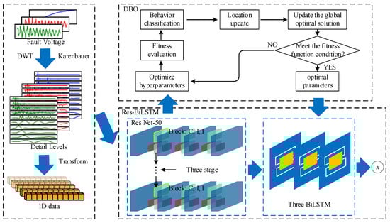
Figure 1. DRB Architecture.

Step 1: Perform Karrenbauer phase-mode transformation on the initial transient voltage traveling wave measured by the fault-location device at the line head to obtain the corresponding modal voltage traveling waves.

Step 2: Extract the wavelet modal maxima of the sum of mode 1 and mode 2 components and the wavelet modal maxima of mode 0 component from the initial transient voltage traveling wave. The ratio of the wavelet modal maxima of the sum of voltage 1-mode and 2-mode to 0-mode is taken as the input feature vector [k₁, k₂, k₃, k₄, k₅, k₆, k₇, k₈, k₉, k₁₀], while the fault distance is used as the output vector. The sample set is divided into a training set and a test set. The training set is fed into the DRB for training.

Step 3: Predict the fault distances for the test set using the trained DRB and evaluate the performance of the model.

3. Results

A 220 kV HVAC transmission line model is built on the PSCAD/EMTDC simulation platform, as shown in Figure 2. The power-frequency line parameters are listed in Table 2. The Frequency Dependent (Phase) Model is adopted. The total length of the HVAC transmission line is 200 km. The fault-location device is installed at the substation. A high sampling rate is employed to accurately capture high-frequency components, with the sampling frequency set to 1 MHz. The simulation time window length is 5 ms, corresponding to 5000 sampling points per channel. The initial transient voltage traveling-wave sample data are collected at the location device.

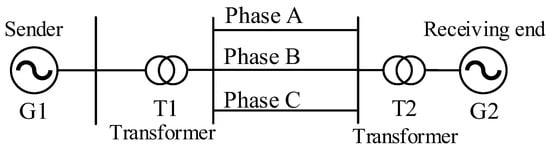
Figure 2. Simplified diagram of a HVAC transmission line.

Table 2. HVAC transmission line parameters.

Ordinal Component	R (Ω/km)	X (Ω/km)	G (S/km)	B (S/km)
Positive sequence	0.0343	0.424	1 × 10−10	2.71 × 10−6
Negative sequence	0.0343	0.424	1 × 10−10	2.71 × 10−6
Zero sequence	0.1800	1.454	1 × 10−10	1.93 × 10−6

A total of 26,026 samples were generated to ensure comprehensive coverage of the fault scenario space. The experimental simulation conditions are set as follows:

(1)

The fault types are single-phase ground fault and two-phase ground fault.

(2)

The fault point was set at distances from the ranging device starting at 5% of the total line length, with a step of 1% and a range from 5% to 95%.

(3)

The transition resistance was varied in steps of 20 Ω, with a range of 0–200 Ω;

(4)

The initial fault phase angle was varied in steps of 30°, covering the range from −60° to 300°.

Each sample contains 10 input variables and 1 output variable. The input feature vector [k₁, k₂, k₃, k₄, k₅, k₆, k₇, k₈, k₉, k₁₀] is constructed from the wavelet modal maxima ratio of the sum of voltage 1-mode and 2-mode to the 0-mode, extracted across 10 consecutive decomposition scales following fault inception. The output variable is the actual fault distance in kilometers.

To ensure the generalization ability of the neural network model and to facilitate hyperparameter tuning and early stopping, the complete dataset was divided into training, validation, and test sets in an 8:1:1 ratio. Specifically, 80% of the samples (20,821 samples) were used for training, 10% (2603 samples) for validation during the DBO optimization and model training process, and the remaining 10% (2602 samples) were held out as a completely independent test set for final performance evaluation. This split strategy provides a robust framework for model development and assessment, and its effectiveness is supported by common practice in machine learning for regression tasks.

3.1. Effect of Transition Resistance Simulation of Positioning Principles

3.1.1. Effect of Transition Resistance

According to Equations (9) and (16), the amplitude ratio of the sum of 1-mode and 2-mode components to the 0-mode component at the fault point is independent of the transition resistance. To verify this conclusion, asymmetric ground faults with the same fault inception angle but different transition resistances of 0 Ω, 100 Ω, and 200 Ω are simulated at a distance of x = 50 km from the measurement point at the line head. The corresponding voltage waveforms are shown in Figure 3.

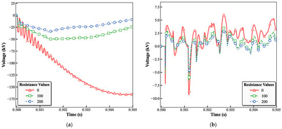
Figure 3. Voltage waveforms of ground faults with different transition resistances at a fault distance of 50 km: (a) Single-phase-to-ground fault; (b) Two-phase-to-ground fault.

As can be observed from Figure 3, when an asymmetric ground fault occurs, different transition resistance values affect the voltage waveform of the faulted phase. The larger the transition resistance, the smaller the amplitude of the voltage waveform, indicating a negative correlation between the two. To further verify this inference, the traveling wave during the fault is subjected to the Karrenbauer transformation to obtain the 0-mode, 1-mode, and 2-mode components of the fault traveling wave. The sum of the 1-mode and 2-mode components and the 0-mode component are then decomposed via wavelet transform, and the amplitude ratios under different transition resistances are compared. The comparison results are shown in Figure 4.

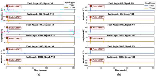
Figure 4. Effect of transition resistance on the d1-scale wavelet modal maxima: (a) Single-phase-to-ground fault; (b) Two-phase-to-ground fault.

As can be seen from Figure 4, under the condition of a constant fault inception angle, the amplitudes of V12 and V0 in a single-phase ground fault are influenced by different transition resistances: the larger the transition resistance, the smaller the amplitudes. However, the ratio of their wavelet modal maxima remains unaffected by changes in the transition resistance. At a distance of 50 km from the measurement point, the ratio of wavelet modal maxima is consistently 1.92. The amplitude ratio pattern for a two-phase ground fault is similar to that of a single-phase ground fault, and its wavelet-modal amplitude ratio is also independent of the transition resistance, with a constant value of 1.61 under the same 50 km condition. Therefore, the inference that the amplitude ratio of the sum of 1-mode and 2-mode components to 0-mode component at the fault point is independent of the transition resistance is verified.

3.1.2. Influence of the Initial Phase Angle of a Fault

According to Equations (9) and (16), the amplitude ratio of the sum of 1-mode and 2-mode components to the 0-mode component at the fault point is independent of the fault inception angle. To verify this inference, fault points with different inception angles are set at a distance of 50 km from the line head for simulation validation. For a single-phase ground fault, as shown in Figure 5a, different fault inception angles cause the wavelet modal maxima of V12 and V0 to vary, but the ratio of the wavelet modal maxima remains identical. This confirms that the fault inception angle does not affect the amplitude ratio of the sum of 1-mode and 2-mode components to the 0-mode component in the case of a single-phase ground fault.

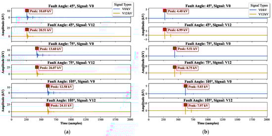
Figure 5. Effect of fault inception angle on the d1-scale wavelet modal maxima: (a) Single-phase-to-ground fault; (b) Two-phase-to-ground fault.

As shown in Figure 5, the amplitude ratio pattern for a two-phase ground fault is the same as that for a single-phase ground fault. Under different fault inception angles, the amplitude ratio of the wavelet modal maxima remains essentially 1.59 at a distance of 50 km from the measurement point, confirming that the fault inception angle does not affect the amplitude ratio of the sum of 1-mode and 2-mode components to the 0-mode component in the case of a two-phase ground fault.

3.1.3. Influence of Fault Distance

As indicated by Equations (11) and (19), once the AC transmission line is specified, its surge impedance and attenuation coefficient become fixed values. Therefore, there exists a corresponding relationship between the distance x from the fault point to the measurement point at the line head and the amplitude ratio of the sum of 1-mode and 2-mode components to the 0-mode component of the voltage at the fault point. To explore this relationship, asymmetric fault points are set along a 200 km AC transmission line, starting from 5 km away from the measurement point with a simulation step of 20 km, covering a range from 5 km to 185 km. This setup is used to investigate how the distance x relates to the amplitude ratio of the sum of the voltage 1-mode and 2-mode components to the 0-mode component at the fault point.

As shown in Figure 6, as the fault distance increases, the amplitude ratio of the sum of 1-mode and 2-mode components to the 0-mode component of the fault-point voltage exhibits a nonlinear increase. Therefore, for an HVAC transmission line with determined parameters, there exists a nonlinear positive correlation between the amplitude ratio of the sum of voltage 1-mode and 2-mode components to the 0-mode component and the fault distance. This nonlinear positive relationship can be regressively fitted using a neural network, thereby enabling fault location for asymmetric faults on HVAC transmission lines.

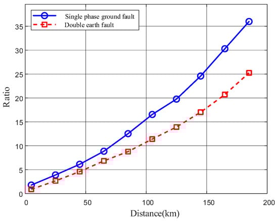
Figure 6. Variation in the amplitude ratio of the sum of 1-mode and 2-mode components to 0-mode component of the fault-point voltage under asymmetric ground faults at different distances.

3.2. Robustness Testing for the DRB Method

To comprehensively evaluate the universality and robustness of the DRB method, this study conducted comparative tests on AC transmission system models featuring a non-transposed transmission line and spanning multiple voltage levels, including 110 kV, 220 kV, and 500 kV. The test results are shown in Figure 7.

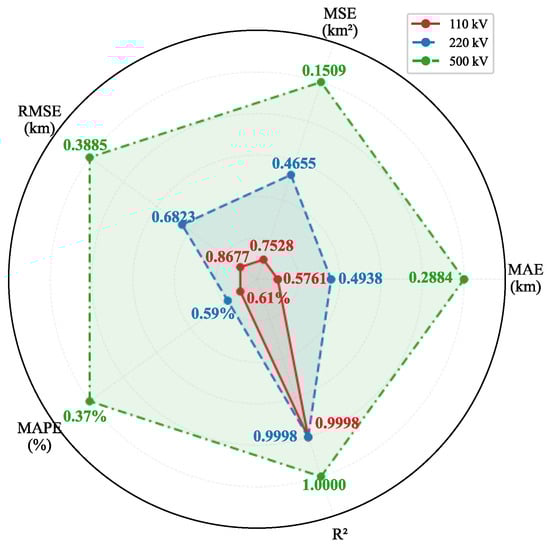
Figure 7. Comparison Chart of Indicators Across Different Voltage Levels.

As shown in Figure 7, the DRB method exhibits good adaptability and stability in all indicators. The experimental results confirm that the performance of the algorithm is not significantly affected by changes in the rated voltage level of the system, and can achieve consistent and effective calculation results over a wide range of tested voltages. Taking a typical 220 kV high-voltage transmission system as an example, to quantitatively evaluate the interference resistance of the assessment method, we injected additional Gaussian white noise at levels of 20 dB, 30 dB, and 40 dB on top of its inherent background noise to simulate actual channel interference of varying intensities. Figure 8 shows a comprehensive performance comparison of this method across different noise levels under 220 kV.

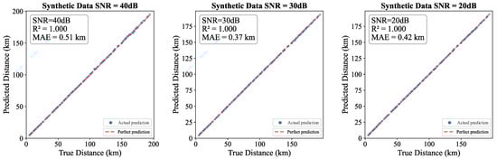
Figure 8. Prediction graph under different noise levels.

As shown in Figure 8, as noise levels increase, prediction accuracy decreases slightly, but the MAE remains below 0.6 km at 40 dB. This demonstrates the DRB’s robust interference resistance. To examine the performance of the DRB network under varying data acquisition precision levels, a comparative experiment across multiple sampling frequencies was conducted. Three representative frequencies were selected: 1 MHz, 700 kHz, and 400 kHz, simulating application scenarios ranging from precision monitoring to cost-effective monitoring. All tests were performed under the same 220 kV transmission system simulation model and a fixed noise level to ensure controlled variables. The results are shown in Table 3.

Table 3. Prediction results at different sampling frequencies.

Frequency	MAE (km)	MSE (km2)	RMSE (km)	MAPE (%)	R2
400 kHz	0.6848	0.8429	0.9883	0.7587	0.9997
700 kHz	0.3668	0.5107	0.4880	0.6312	0.9999
1 MHz	0.3648	0.4396	0.5489	0.4403	0.9999

According to Table 3, increasing the sampling frequency can improve the prediction accuracy, and the model exhibits strong fitting ability above 400 kHz, but there is a marginal decreasing effect.

3.3. Ablation Study

To quantitatively evaluate the contribution of each proposed module in the DRB, a systematic ablation study was conducted. Four model variants were compared: (1) Base LSTM (the baseline); (2) BiLSTM (incorporating bidirectional structure); (3) Res-BiLSTM (further adding residual connections); and (4) DBO-Res-BiLSTM (the complete proposed model with DBO optimization). All experiments were performed on the same dataset with identical splits, using MAE, RMSE, and MAPE as evaluation metrics. The results are summarized in Table 4.

Table 4. Comparison of Melting Experiment Results.

	LSTM	BiLSTM	Res	DBO	MAE (km)	RMSE (km)	MAPE (%)
1	√				2.1538	2.7921	2.4169
2		√			1.5192	1.7924	1.6827
3		√	√		0.7841	1.0217	0.8529
4		√	√	√	0.3950	0.5163	0.4149

As shown in Table 4, a progressive performance improvement is observed from the Base LSTM to the complete DRB model, with all error metrics consistently decreasing across variants: (1) The BiLSTM reduced RMSE by 35.8% versus Base LSTM, confirming bidirectional encoding better captures temporal context. (2) Adding residual connections further lowered RMSE by 43.0%, showing the residual structure mitigates gradient issues and aids feature reuse. (3) DBO optimization cut RMSE by another 49.5%, validating its role in automating hyperparameter search and avoiding manual tuning limits.

The ablation study systematically confirms the individual contributions and synergistic effects of the three modules: the bidirectional structure, residual connections, and the DBO optimization algorithm.

3.4. Performance Comparison of the DRB with Other Methods

To validate the fault location capability of DRB in HVAC transmission lines, it was compared with the CNN-LSTM location algorithm, the Transformer location algorithm, and the traditional Type-A traveling wave method.

Based on the line parameters in Table 2, the line-mode traveling-wave velocity is approximated as $v_1\approx 1/\sqrt{LC}$ km/s = 2.93145 × 10⁵ km/s. The conventional single-ended Type-A traveling-wave method requires collecting the arrival time of the initial voltage traveling-wavefront and the arrival time of the second reflected wavefront for location. The identification of the second reflected wavefront can be achieved by distinguishing the polarities of the fault-point reflected wavefront and the remote-bus reflected wavefront. According to the Type-A traveling-wave location formula in reference [25], the fault distance can then be calculated.

As shown in Figure 9 and Table 5, The systematic evaluation in this study demonstrates that among the four predictive models (DRB, CNN-LSTM, Transformer, and Type-A), the proposed DRB model achieves the best overall performance. It obtains the minimum values across all error metrics (MAE: 0.3648; MSE: 0.4396; RMSE: 0.5489; MAPE: 0.4403%) and the highest coefficient of determination R² of 0.9999, reflecting its superior prediction accuracy, stability, and goodness-of-fit. The CNN-LSTM and Transformer models perform comparably and significantly outperform the conventional baseline model Type-A, confirming the effectiveness of deep hybrid architectures and attention mechanisms for the present task. In contrast, the Type-A model shows clear gaps across all metrics, highlighting the necessity of adopting advanced model architectures.

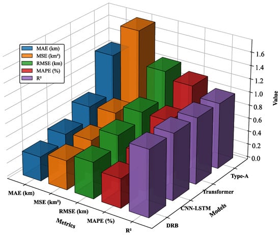
Figure 9. Evaluation Indices of Different Methods.

Table 5. Partial prediction results for each algorithm at different voltage levels.

Model	MAE (km)	MSE (km2)	RMSE (km)	MAPE (%)	R2
DRB	0.3648	0.4396	0.5489	0.4403	0.9999
CNN-LSTM	0.4791	0.5124	0.7158	0.57	0.9998
Transformer	0.6800	0.7047	0.8395	0.83	0.9998
Type-A	1.2643	1.7486	1.2444	1.14	0.9933

4. Discussion

The fault location method proposed in this paper utilizes the mode amplitude ratio of traveling wave modes combined with deep learning to establish a stable nonlinear mapping between the fault distance and the amplitude ratio of the sum of voltage 1-mode and 2-mode to the 0-mode. Both theoretical derivation and simulation verify that this ratio is theoretically independent of transition resistance and fault inception angle, effectively overcoming the limitations of traditional impedance-based and traveling-wave methods, which are sensitive to transition resistance and require the identification of reflected wavefronts.

This method innovatively transforms the dispersion characteristics of traveling waves from error sources to the basis for localization. Extracting modal amplitude features through the wavelet transform avoids the need for wave velocity estimation and reflection wave recognition. Compared with traditional traveling wave methods and other deep learning networks, it has higher convergence speed, generalization ability, and accuracy.

It is important to address the assumptions made in the theoretical derivation regarding line parameters. Equations (9), (16) and (19) are derived under the assumption that line parameters (such as Z₀, Z₁, Z₂ and α₀, α₁) are constants. In reality, transmission line parameters—particularly the zero-mode components—are frequency-dependent due to the skin effect and ground-return effect. However, the proposed method focuses on the initial transient voltage wavefront, the energy of which is primarily concentrated within a specific high-frequency range (typically tens to hundreds of kHz). Within this dominant frequency band, the variation in parameters is relatively smooth, allowing for the use of effective parameter values. Furthermore, the use of the amplitude ratio (1-mode and 2-mode versus 0-mode) partially mitigates the sensitivity to absolute parameter variations. Most importantly, the data-driven nature of the DRB model allows it to learn the complex, non-linear mapping relationships that exist in real-world scenarios, thereby compensating for the theoretical simplifications of the constant-parameter model.

Despite these advantages, the method presents certain limitations and implementation risks. Firstly, its core principle relies on the zero-sequence mode component generated by ground faults; therefore, it is not directly applicable to fault types that do not produce this component, such as phase-to-phase faults. Secondly, in practical applications, measurement noise, sensor frequency response characteristics, sampling synchronization errors, as well as complex grid conditions (e.g., non-uniform transposition, multi-branch configurations, and hybrid lines) may affect the accuracy of modal decomposition and introduce location errors. Additionally, the DRB model relies on extensive datasets for training, and its online performance depends on the coverage of the training data. Re-training or fine-tuning may be required for lines with entirely new topologies or significantly different parameters.

Compared to existing methods, the strength of the proposed approach lies in its principled avoidance of two major error sources—wave velocity estimation and reflected wave identification—and its inherent robustness to high-impedance ground faults. Its weakness, however, is the current limitation to ground faults and its dependency on data quality. Traditional traveling-wave methods, while susceptible to wave velocity errors, are in principle applicable to various fault types. Methods based on high-frequency inherent frequencies, although independent of wave velocity, are significantly influenced by line boundary reflections.

Although the current method is designed for ground faults, its fundamental principle holds potential for extension to other fault types. For instance, for phase-to-phase faults, future research could explore constructing new feature quantities using the amplitude or phase relationships between positive- and negative-sequence modes. Future work will focus on developing an adaptive fault-type identification and mode selection mechanism that automatically chooses the most effective modal combination based on the characteristics of the initial traveling wave, thereby extending the applicability of this method to a broader range of fault scenarios.

In summary, this method offers an effective approach to fault location based on the fusion of data-driven techniques and physical characteristics, contributing to the advancement of smarter and more robust fault localization in power systems. Future research will continue in three main directions: deepening the theoretical generality (including frequency-dependent modeling), enhancing engineering practicality, and expanding the range of applicable scenarios.

5. Conclusions

Aiming at the problems existing in single-ended traveling-wave fault location methods for asymmetric ground faults on HVAC transmission lines, this paper proposes a single-ended location method based on the modal amplitude ratio by utilizing the traveling-wave dispersion characteristics. The method features fast computation, good robustness, and strong generalization capability. Through theoretical analysis and simulation verification, the following conclusions are drawn.

(1)

The relationship between the fault distance and the amplitude ratio of the sum of 1-mode and 2-mode components to the 0-mode component of the initial transient voltage traveling wave at the measurement point is a definite nonlinear mapping, which is independent of the transition resistance and the fault inception angle.

(2)

In the high-frequency range, the relationship between the fault distance and the wavelet modal maximum ratio of the sum of voltage 1-mode and 2-mode components to the 0-mode component approximates a stable nonlinear curve.

(3)

Compared with the conventional single-ended traveling-wave location method, the proposed method achieves higher accuracy without the need to identify the reflected wavefront. It also surpasses traditional neural-network-based location models in accuracy. Moreover, its location capability is unaffected by fault type, fault location, transition resistance, or fault inception angle.

References

- Li, J.M.; Chu, S.C.; Shao, X.; Pan, J.-S. A single-phase-to-ground fault location method based on convolutional deep belief network. Electr. Power Syst. Res. 2022, 209, 108044. [Google Scholar]
- Naidu, O.D.; Pradhan, A.K. Precise traveling wave-based transmission line fault location method using single-ended data. IEEE Trans. Ind. Inform. 2020, 17, 5197–5207. [Google Scholar] [CrossRef]
- Zhu, B.; Yu, C.; Ma, J. Wavefront steepness based single-ended traveling wave fault location for transmission lines. Autom. Electr. Power Syst. 2021, 45, 130–135. [Google Scholar]
- Fayazi, M.; Joorabian, M.; Saffarian, A.; Monadi, M. A single-ended traveling wave based fault location method using DWT in hybrid parallel HVAC/HVDC overhead transmission lines on the same tower. Electr. Power Syst. Res. 2023, 220, 109302. [Google Scholar] [CrossRef]
- Zhang, M.; Zhao, W.; Li, P. Two-terminal fault combination location method on MMC-HVDC transmission lines based on ensemble empirical mode decomposition. Energy Rep. 2023, 9, 987–995. [Google Scholar] [CrossRef]
- Yang, Y.; Huang, C.; Zhou, D.; Li, Y. Fault detection and location in multi-terminal DC microgrid based on local measurement. Electr. Power Syst. Res. 2021, 194, 107047. [Google Scholar] [CrossRef]
- Luo, J.; Liu, Y.; Cui, Q.; Zhong, J.; Zhang, L. Single-ended time domain fault location based on transient signal measurements of transmission lines. Prot. Control. Mod. Power Syst. 2024, 9, 61–74. [Google Scholar] [CrossRef]
- Bai, H.; Hong, Z. A fault traveling wave location method based on CEEMD and NTEO. Power Syst. Prot. Control. 2022, 50, 50–59. [Google Scholar]
- Yu, K.; Zeng, J.; Zeng, X.; Xu, F.; Ye, Y.; Ni, Y. A novel traveling wave fault location method for transmission network based on directed tree model and linear fitting. IEEE Access 2020, 8, 122610–122625. [Google Scholar] [CrossRef]
- Jiang, K.; Zhou, K.; Ren, X.; Xu, Y. Frequency Domain Sampling Optimization of Cable Defect Detection and Location Method Based on Exponentially Increased Frequency Reflection Coefficient Spectrum. Energies 2025, 18, 2428. [Google Scholar] [CrossRef]
- Meng, P.; Li, T.; Zhou, K.; Tang, Z.; Zhu, G.; Li, Z.; Cao, Y.; Zhang, H.; Yin, Y.; Guo, J. A Novel Time–Frequency-Domain Reflectometry Location Method for Power Cable Defects Based on Synchrosqueezing Transform. IEEE Trans. Instrum. Meas. 2024, 73, 1–9. [Google Scholar] [CrossRef]
- Xia, Y.; Li, Z.; Xi, Y.; Wu, G.; Peng, W.; Mu, L. Accurate fault location method for multiple faults in transmission networks using travelling waves. IEEE Trans. Ind. Inform. 2024, 20, 8717–8728. [Google Scholar] [CrossRef]
- Rezaei, D.; Gholipour, M.; Parvaresh, F. A single-ended traveling-wave-based fault location for a hybrid transmission line using detected arrival times and TW’s polarity. Electr. Power Syst. Res. 2022, 210, 108058. [Google Scholar] [CrossRef]
- Hudomalj, M.; Trost, A.; Čampa, A. Traveling wave method for event localization and characterization of power transmission lines. Electr. Power Syst. Res. 2024, 232, 110382. [Google Scholar] [CrossRef]
- Zeng, R.; Wu, Q.; Zhang, L. Two-terminal traveling wave fault location based on successive variational mode decomposition and frequency-dependent propagation velocity. Electr. Power Syst. Res. 2022, 213, 108768. [Google Scholar] [CrossRef]
- Gao, S.; Xu, Z.; Song, G.; Shao, M.; Jiang, Y. Fault location of hybrid three-terminal HVDC transmission line based on improved LMD. Electr. Power Syst. Res. 2021, 201, 107550. [Google Scholar] [CrossRef]
- Zhu, Y.; Peng, H. Multiple random forests based intelligent location of single-phase grounding fault in power lines of DFIG-based wind farm. J. Mod. Power Syst. Clean Energy 2022, 10, 1152–1163. [Google Scholar] [CrossRef]
- Wang, X.; Zhou, P.; Peng, X.; Wu, Z.; Yuan, H. Fault location of transmission line based on CNN-LSTM double-ended combined model. Energy Rep. 2022, 8, 781–791. [Google Scholar] [CrossRef]
- Wu, K.; Xu, C.; Yan, J.; Wang, F.; Lin, Z.; Zhou, T. Error-distribution-free kernel extreme learning machine for traffic flow forecasting. Eng. Appl. Artif. Intell. 2023, 123, 106411. [Google Scholar] [CrossRef]
- Li, Y.; Chen, Y.; Deng, F. High Impedance Fault Detection Method Based on Traveling Wave Full Waveform Fault Characteristics. In Proceedings of the 2023 IEEE International Conference on Advanced Power System Automation and Protection (APAP), Xuchang, China, 8–12 October 2023. [Google Scholar]
- Deng, F.; Wang, Z.; Li, T.; Zhong, H.; Wang, R. Accurate Fault Location Method for Distribution Network Based on Spatio-Temporal Panoramic Information. In Proceedings of the 2025 IEEE 8th International Electrical and Energy Conference (CIEEC), Changsha, China, 16–18 May 2025. [Google Scholar]
- Shafiq, M.; Gu, Z. Deep residual learning for image recognition: A survey. Appl. Sci. 2022, 12, 8972. [Google Scholar] [CrossRef]
- Siami-Namini, S.; Tavakoli, N.; Namin, A.S. The performance of LSTM and BiLSTM in forecasting time series. In Proceedings of the 2019 IEEE International Conference on Big Data (Big Data), Los Angeles, CA, USA, 9–12 December 2019. [Google Scholar]
- Xue, J.; Shen, B. Dung beetle optimizer: A new meta-heuristic algorithm for global optimization. J. Supercomput. 2023, 79, 7305–7336. [Google Scholar] [CrossRef]
- Chen, P.; Xu, B.; Li, J. The optimized combination of fault location technology based on traveling wave principle. In Proceedings of the 2009 Asia-Pacific Power and Energy Engineering Conference, Wuhan, China, 27–31 March 2009. [Google Scholar]
Disclaimer/Publisher’s Note: The statements, opinions and data contained in all publications are solely those of the individual author(s) and contributor(s) and not of MDPI and/or the editor(s). MDPI and/or the editor(s) disclaim responsibility for any injury to people or property resulting from any ideas, methods, instructions or products referred to in the content. |
© 2026 by the authors. Licensee MDPI, Basel, Switzerland. This article is an open access article distributed under the terms and conditions of the Creative Commons Attribution (CC BY) license.