A Missing Data Imputation Method for Distribution Network Data Based on TGAN-GP

Abstract

Distribution network data may encounter random missing data caused by abnormal conditions and continuous missing data caused by natural disasters during gathering, transmission, and conversion. To address these problems, this paper proposes a missing data imputation method based on the Temporal Generative Adversarial Network with Gradient Penalty (TGAN-GP), which takes the Wasserstein Generative Adversarial Network with Gradient Penalty (WGAN-GP) as its basic framework, replaces traditional fully connected layers with a Temporal Convolutional Network (TCN) in the generator’s core, leverages causal dilated convolution to efficiently capture the long-range temporal dependencies and periodicity of measurement data, and integrates residual connections to mitigate gradient vanishing and network degradation during deep training. For the discriminator, the method adopts a Long Short-Term Memory (LSTM) network, which enhances the evaluation of the temporal rationality of generated data and thereby further improves imputation accuracy. Finally, simulations were conducted on the IEEE 33-bus distribution network test system. Results show that under the random missing scenario (10% missing rate), the Root Mean Squared Error (RMSE) and Mean Absolute Error (MAE) of node voltage magnitude imputation are as low as 0.00062 and 0.00051, those of node injected active power imputation are 0.00081 and 0.00065, and those of node injected reactive power imputation are 0.00082 and 0.00076. Under the continuous missing scenario, the RMSE and MAE of node voltage magnitude imputation are 0.00147 and 0.00122, those of node injected active power imputation are 0.00373 and 0.00268, and those of node injected reactive power imputation are 0.00314 and 0.00226. The imputation errors of all three data types are significantly lower than the comparison methods’.

1. Introduction

The widespread integration of distributed energy resources (DERs) and electric vehicles (EVs) is profoundly transforming distribution network operations, greatly increasing measurement data complexity and challenging its effective representation [1,2]. Additionally, large-scale new loads raise grid operational uncertainty, simplifying to more complex measurement data analysis. When the distribution network experiences anomalies or disruptions due to disasters, resulting in missing data, it can compromise data quality and the estimation of grid status [3]. Therefore, research on more accurate missing measurement data imputation methods matters greatly for boosting Distribution System State Estimation (DSSE) precision [4,5].

Extensive global research on measurement data missing imputation identifies three main categories. The first method is direct deletion. Although it can quickly handle missing data, there is a risk of losing crucial data, so it is rarely used [6]. The second category involves statistical methods, such as imputation using mean, mode, and median [7]. These methods only consider data’s statistical characteristics, ignoring temporal and relational aspects, leading to large imputation errors. The third category includes machine learning-based methods such as Random Forests (RF) [8], K-Nearest Neighbor (KNN) [9], Support Vector Machines (SVM) [10,11], and Matrix Factorization [12,13]. However, traditional machine learning cannot capture deep data structures, especially in time-series data of distribution networks, resulting in inefficient interpolation. Therefore, this paper proposes an electrical measurement data interpolation method based on deep learning. Refs [14,15] adopted Long Short-Term Memory (LSTM) networks for missing data imputation. However, using time-step recursive sequence processing can make parallel computing difficult and reduce the efficiency of long sequence imputation.

In 2014, Goodfellow proposed a Generative Adversarial Network (GAN) [16]. Due to efficient generation and feature learning capabilities, GAN has gained wide recognition in image processing [17,18,19,20,21]. Recently, GANs have also been successfully applied to sample generation in other fields [22,23,24,25,26,27]. Wang et al. [28] replaced JS divergence with Wasserstein divergence to form a WGAN for power system data reconstruction. However, WGAN’s weight clipping may cause gradient vanishing/explosion during training. Meanwhile, electrical loads are time-dependent [29], and GANs alone may miss the grid data’s temporal information.

Addressing the limitations of existing missing data imputation methods, such as unstable training of GANs and poor performance on long-term sequences, this paper proposes a TGAN-GP method. Its main contributions and innovations are as follows:

(1)

Firstly, WGAN-GP is adopted as the basic framework to replace the traditional GAN. It employs a gradient penalty strategy instead of a weight clipping mechanism, thereby enhancing the stability of model training.

(2)

Secondly, the generator employs a TCN, which utilizes parallel convolution and long-range dependency capture to enhance the accuracy of long-term sequence reconstruction. Furthermore, through residual connections, it mitigates the degradation of deep networks during training and improves the stability of high-dimensional nonlinear time series power data.

(3)

Thirdly, LSTM is selected as the discriminator. Its ability to capture long-term and short-term dependencies in data enables accurate identification of temporal correlations in time series, effectively distinguishing potential logical deviations between real data and generator input data, thereby improving the output quality of the generator.

The remainder of this paper is organized as follows: Section 2 presents the research background. Section 3 presents the detailed design of the TGAN-GP model and the data imputation steps. Section 4 and Section 5 present the experimental design and result analysis. Section 6 gives concluding remarks and outlines future research directions.

2. Research Background

In the actual operation of distribution networks, measurement data are often missing, which leads to a decline in system observability [30]. The causes of missing data can be categorized into two types, as illustrated in Figure 1. Therefore, this paper presents the TGAN-GP method to resolve this issue.

(1)

Random Missing Measurement Data: This features scattered temporal and spatial distribution, primarily due to transient, sporadic factors. For instance, temporary sensor failures, occasional data acquisition module glitches, or unstable communication links (e.g., wireless electromagnetic interference, poor wired contact) may interrupt recording or cause time-specific packet loss, resulting in discrete, irregular missing data.

(2)

Continuous Missing Measurement Data: This type of missing data involves continuous-time data interruptions in specific regions, mainly triggered by persistent faults or systemic events (e.g., device damage from lightning/heavy rain, prolonged base station power outages, broken backbone cables). It typically covers a large range and lasts for extended periods, spanning multiple complete time segments.

3. Overall Framework of the TGAN-GP Model

3.1. WGAN-GP Model

A Generative Adversarial Network (GAN) is a deep learning generative network composed of two neural networks: a generator (G) and a discriminator (D) [31,32]. Via adversarial learning between the two components, the model ultimately achieves Nash equilibrium. The structural model of GAN can be seen in Figure 2. As illustrated, historical measurement data collected from the distribution network act as real samples (denoted as x) that follow the real data distribution. The generator’s input is random noise from a standard normal distribution, and it outputs generated data with a distribution that is close to the real samples’ distribution. The discriminator receives real and generated samples, outputs the input’s probability of being a real sample to distinguish them, and feeds back the discrimination result to synchronously optimize generator and discriminator parameters for their adversarial collaborative training.

The generator minimizes its loss to maximize the discriminator’s output (denoted as $L_G$) to generate more realistic data, while the discriminator minimizes its own loss (denoted as $L_D$) to distinguish between real and generated data. Their loss functions are as follows:

$$L_G=-E_{z~p_z(z)}[\log D(G(z))]$$

(1)

$$L_D=-E_{x~p_{\mathrm{r}}(x)}\left[\log D(x)\right]-E_{z~p_z(z)}\left[\log (1-D(G\left(z\right)))\right]$$

(2)

where, $E$ represents the expectation distribution, $G\left(z\right)$ represents the data generated by the Generator, and $D(~)$ represents the discriminator output.

The generator and discriminator form a minimax game, so the final GAN objective function is as follows:

$$\underset{G}{\min } \underset{D}{\max }V\left(D,G\right)=E_{x~p_r\left(x\right)}\left[\log D\left(x\right)\right]+E_{z~p_z\left(z\right)}\left[\log (1-D\left(G\left(z\right)\right))\right]$$

(3)

However, the loss function of traditional GAN uses log cross-entropy to measure the difference between generated data and real data, which often leads to issues such as gradient vanishing and training instability. Therefore, the Wasserstein distance is used to replace cross-entropy loss for measuring the difference between the probability distributions of generated data and real data. Meanwhile, the objective function of the WGAN is defined as follows:

$$\underset{G}{\min } \underset{D}{\max }V\left(D,G\right)=E_{x~p_r\left(x\right)}\left[D\left(x\right)\right]-E_{z~p_z\left(z\right)}\left[D\left(G\left(z\right)\right)\right]$$

(4)

The WGAN-GP proposed in this paper further improves the 1-Lipschitz constraint method of the discriminator based on the original WGAN. Unlike the original WGAN, which employs weight clipping, WGAN-GP introduces a gradient penalty term at interpolation points between real and generated samples, making the discriminator gradient norm close to 1, thus satisfying the 1-Lipschitz condition in a smoother and more effective way. At this point, the objective function of WGAN-GP is redefined as follows:

$$\begin{array}{l}\underset{G}{\min } \underset{D}{\max }V\left(D,G\right)=E_{x~p_r\left(x\right)}\left[D\left(x\right)\right]-\\ E_{z~p_z\left(z\right)}\left[D\left(G\left(z\right)\right)\right]+\lambda E\left[{\left({‖\nabla D\left(x^{\prime }\right)‖}_2-1\right)}^2\right]\end{array}$$

(5)

In Equation (5), $\lambda E\left[{\left({‖\nabla D\left(x^{\prime }\right)‖}_2-1\right)}^2\right]$ represents the gradient penalty term, and $\lambda$ represents the weight coefficient of the gradient penalty term. $x^{\prime }$ denotes the randomly linearly interpolated sample between real data and generated data, with the expression $x^{\prime }=\epsilon x+\left(1-\epsilon \right)G\left(z\right), \epsilon \in \left(0,1\right)$, $\nabla D\left(x^{\prime }\right)$ represents the gradient of the discriminator with respect to the interpolated sample.

3.2. TCN Model

TCN is a convolutional neural network for time-series modeling, composed of causal convolution, dilated convolution, and residual connections [33]. Due to the large time span of SCADA measurement data, TCN is selected as the generator in WGAN-GP, showing better performance than fully connected networks in long-time-series data generation.

Causal convolution limits the convolution kernel’s receptive field to current and historical time steps, ensuring temporal causality in time-series generation. Dilated convolution expands the receptive field exponentially via a dilation factor between kernel sampling points, supporting long-range dependency modeling without significant increases in network depth or computational load.

Causal and dilated convolutions are combined, and their structure is shown in Figure 3. It is defined as follows:

$$y(t)={\displaystyle \sum _{j=0}^{k-1}h\left(j\right)·x\left(t-d·j\right)}$$

(6)

where $y(t)$ represents the output at time t, $h\left(j\right)$ represents the j-th weight of the convolution kernel, $x\left(t-d·j\right)$ represents the data sampled by skipping d steps in the input sequence, k represents the size of the convolution kernel, taking a value of 3, d represents the dilation factor, taking a value of 1 for ordinary causal convolution; and a dilation operation is introduced when $d>1$.

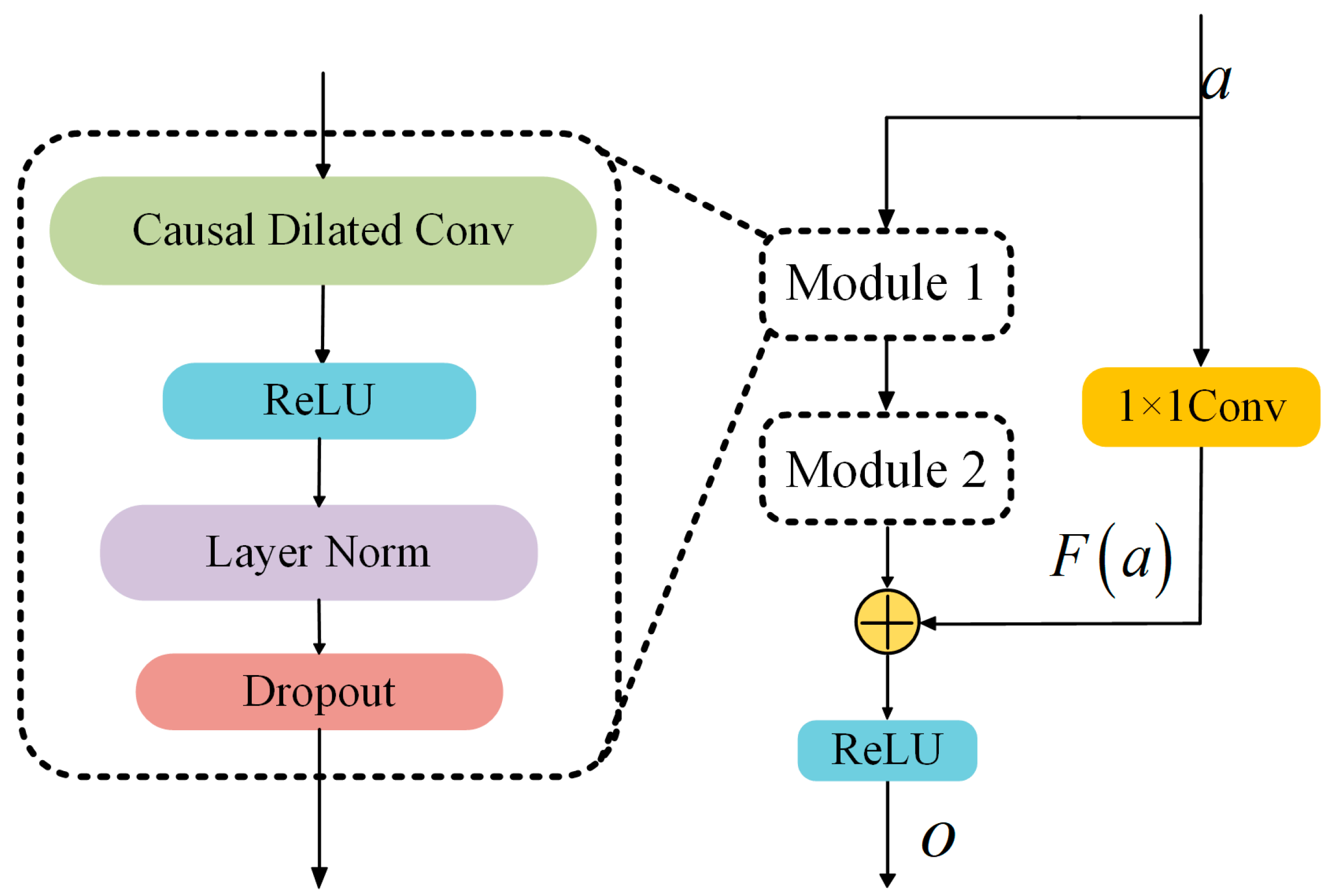
The residual block introduces residual connections into the network structure, and its mathematical definition is as follows:

$$o=\mathit{ReLU}\left(F\left(a\right)+a\right)$$

(7)

where $a$ represents the input feature, $F\left(·\right)$ represents the nonlinear transformation applied to the input, $o$ represents the output feature.

The structure of the residual block is shown in Figure 4.

3.3. LSTM Model

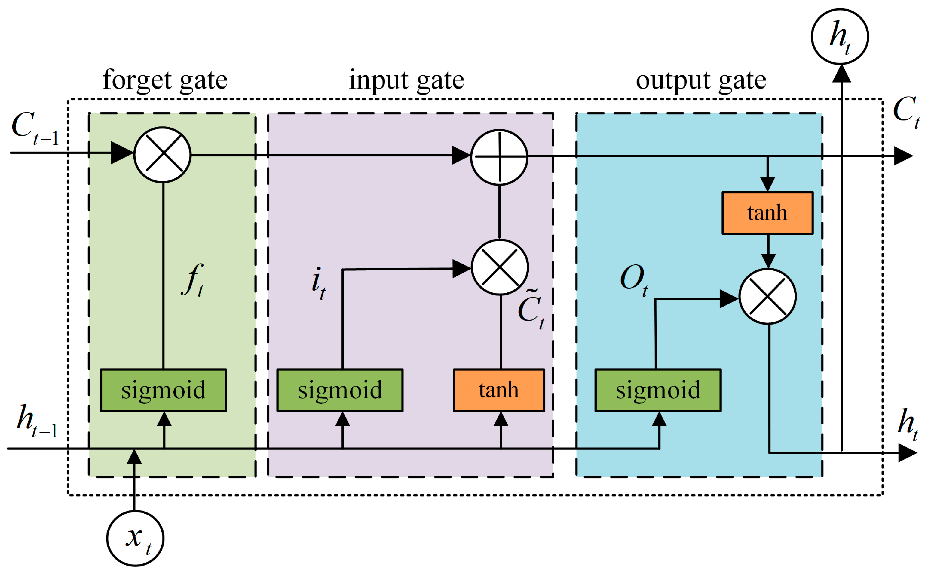
LSTM is a type of recurrent neural network, suitable for handling long and short-term dependencies in time series data. As a discriminator in GAN, it leverages its strengths in time series modeling to learn the temporal differences between generated data and real data, enabling effective classification. Its structure (as shown in Figure 5) consists of a forget gate, an input gate, and an output gate.

The updated formulas for the three gates are as follows:

$$\left\{\begin{array}{l}{f}_t=\sigma \left(W_f·\left[h_{t-1},x_t\right]+b_f\right)\\ i_t=\sigma \left(W_i·\left[h_{t-1},x_t\right]+b_i\right)\\ O_t=\sigma \left(W_o·\left[h_{t-1},x_t\right]+b_o\right)\\ {\tilde{C}}_t=\tanh \left(W_C·\left[h_{t-1},x_t\right]+b_C\right)\\ h_t=O_t·\tanh \left(C_t\right)\\ C_t=f_t·C_{t-1}+i_t·{\tilde{C}}_t\end{array}\right.$$

(8)

where, $W_f$, $W_i$, $W_o$ and $W_C$ represent the weight matrices of the forget gate, input gate, output gate, and candidate memory cell, respectively; $\sigma$ represents the sigmoid activation function; $\tanh$ represents the hyperbolic tangent activation function; $b_f$, $b_i$, $b_o$ and $b_C$ represent the corresponding bias terms.

3.4. Integration and Training Process of the TGAN-GP Model

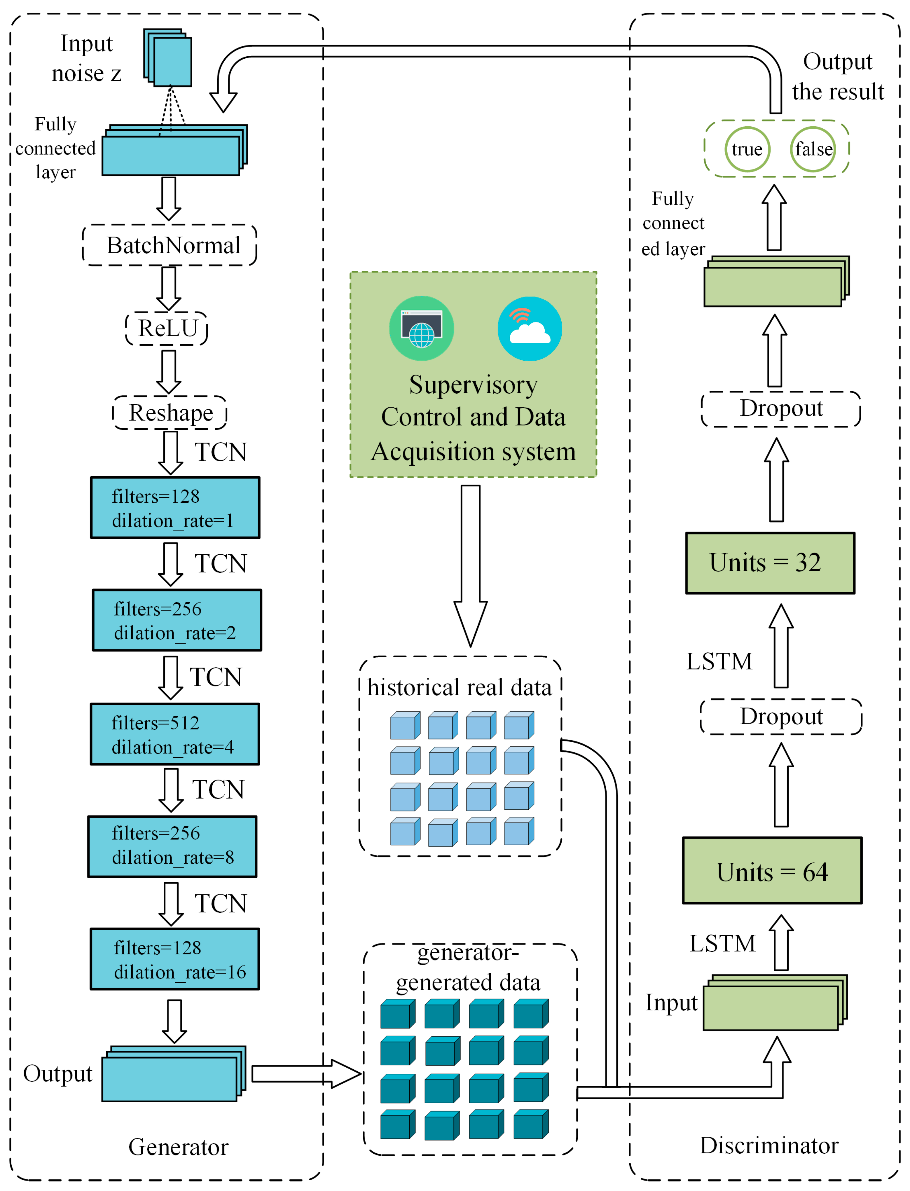
Figure 6 illustrates the model training process. In each adversarial training round, the generator learns measurement data temporal features via TCN to generate real-approximating data; the discriminator takes generated and historical real data as inputs, discriminates via an LSTM network, calculates loss, and feeds it back to the generator for iterative optimization. This proceeds until the discriminator fails to distinguish the two, yielding generated data (denoted as $G\left(z\right)$) with a nearly identical distribution to real data. The generator comprises multiple TCN residual blocks: firstly, a fully connected layer expands the noise vector to a specified dimension, then five TCN residual blocks follow in sequence (dilation factors: 1, 2, 4, 8, 16; channel numbers: 128 → 256 → 512 → 256 → 128). The discriminator has two LSTM layers (64 and 32 hidden units, respectively) and outputs a single discrimination value through a fully connected layer to provide generator feedback.

3.5. Data Imputation Steps

Utilizing data generated by the TGAN-GP model to effectively fill in missing positions, a method based on Euclidean distance was designed for filling [34]. The specific steps are as follows:

Firstly, construct a binary mask matrix B matching the historical measurement data matrix in dimensions, then compute the two matrices’ Hadamard product to get a matrix with missing data, expressed as follows:

$$\overline{X}=X\odot B$$

(9)

where B represents a binary mask matrix with the same dimensions as the test set, where a value of 1 indicates normal data and 0 indicates missing data. $\odot$ represents the Hadamard product operation.

Secondly, the generated data were used to fill in the missing positions. After completing the imputation, the complete data matrix $\widehat{X}$ is obtained as follows:

$$\widehat{X}=\overline{X}+(1-B)\odot G\left(z\right)$$

(10)

It can be seen from the above formula that the filled data includes both original non-missing data and generated data for missing positions.

4. Experimental Preparation

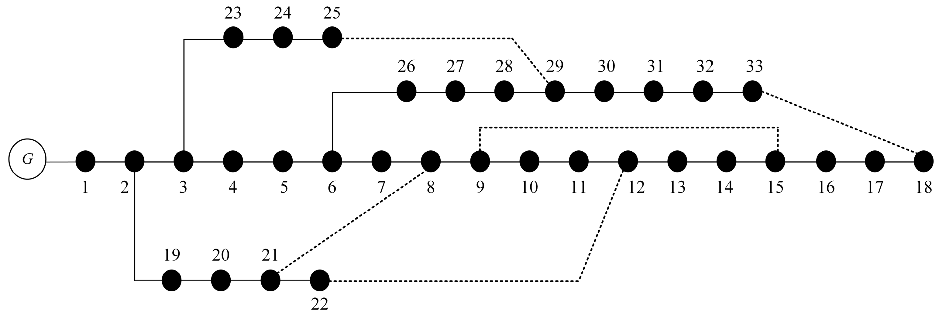
The experimental computing environment and implementation details are as follows: Hardware: Experiments ran on a workstation with an Intel (R) Core (TM) i5-8500 CPU (3.00 GHz) and 32.0 GB RAM; Software: The operating system was Microsoft Windows, and the algorithm was implemented in Python 3.9 based on the TensorFlow 2.10.0 framework; Test system: The IEEE 33-bus test system was used (with its topology shown in Figure 7) [35].

4.1. Experimental Dataset

In practical applications, missing measurement data are unavailable, so the effectiveness of imputation cannot be directly assessed with true values, which makes the problem essentially unsupervised [36]. This paper uses a complete, reliable dataset to artificially generate one with missing values, then compares imputed (reconstructed) data with the original complete dataset to evaluate the proposed method. Thus, the dataset was not split into training and testing sets, as validation relies on comparing imputed results with the original data, obviating the need for an independent test set.

The experimental dataset is derived from the load data of a specific region under the NYISO jurisdiction. The data used are the load information for June, with a sampling interval of 5 min, totaling 8640 sample groups. Each sample group includes: node voltage amplitude measured by the SCADA system, active and reactive power injected into nodes, and active and reactive power flows of branches. The dimensionality of the dataset used in this paper for training was (8640, 33, 3), where 8640 represents the number of samples, 33 denotes the number of nodes, and 3 corresponds to the number of features (voltage amplitude, active power, reactive power).

Considering the inevitability of noise in the actual measurement environment, during the simulation process, we incorporate Gaussian noise with a mean of 0 and a standard deviation of 0.001 into the SCADA measurement data to simulate real-world measurement scenarios.

4.2. Error Evaluation Metrics

To verify the effectiveness of the proposed imputation method quantitatively, the Root Mean Squared Error (RMSE) and Mean Absolute Error (MAE) are used as error evaluation indicators to assess the error between the algorithm-derived imputed values and the true values. The formula is defined as follows:

$$\mathit{RMSE}=\sqrt{{\displaystyle \frac{1}{n}}{\displaystyle \sum _{i=1}^n{(y_i-{\widehat{y}}_i)}^2}}$$

(11)

$$\mathit{MAE}={\displaystyle \frac{1}{n}}{\displaystyle \sum _{i=1}^n\left|y_i-{\widehat{y}}_i\right|}$$

(12)

where, $y_i$ is the true value at the i-th position, ${\widehat{y}}_i$ is the imputed value, and n is the total number of missing nodes. RMSE calculates the average of squared differences between imputed and true values, being more sensitive to large errors. MAE measures their average absolute difference, thus being relatively stable. For both indicators, smaller values indicate more ideal imputation effects.

4.3. Training Settings

The model is trained for 100 epochs (34 min total) with a batch size of 32, gradient penalty λ = 17.5, and Adam optimizer (fixed initial learning rates: 0.00001 for generator, 0.00005 for discriminator; β₁ = 0.5, β₂ = 0.9). It underwent 500 rounds of adversarial training with the objective function in Equation (5).

5. Case Study

5.1. Results of Random Missing Measurement Data Imputation

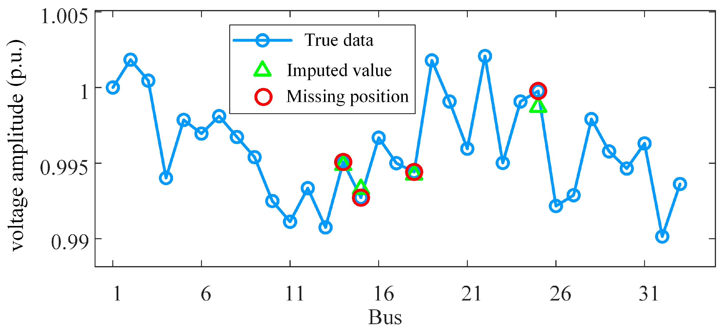
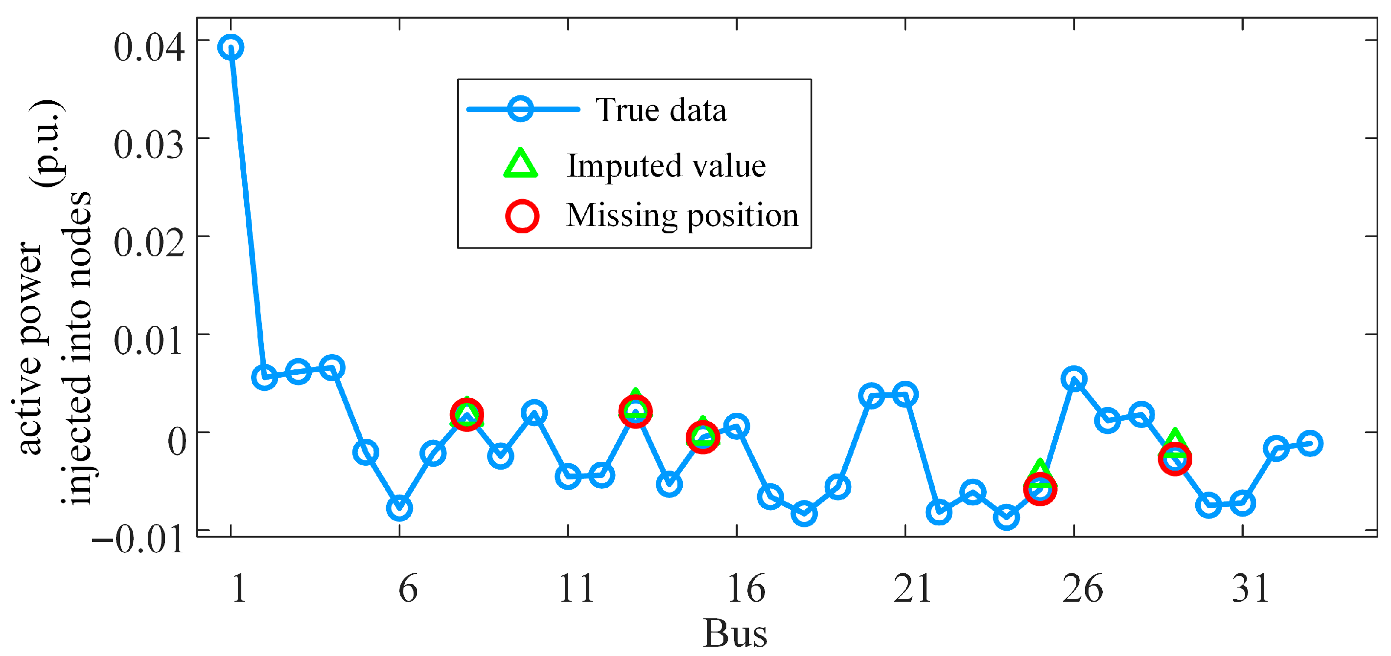
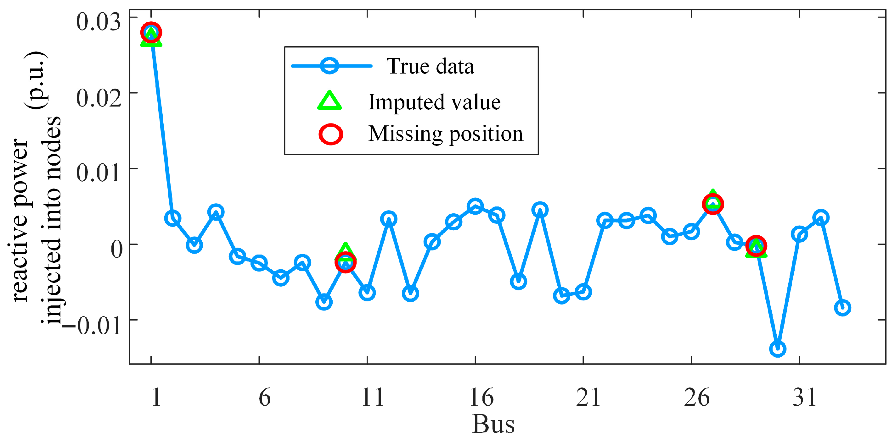
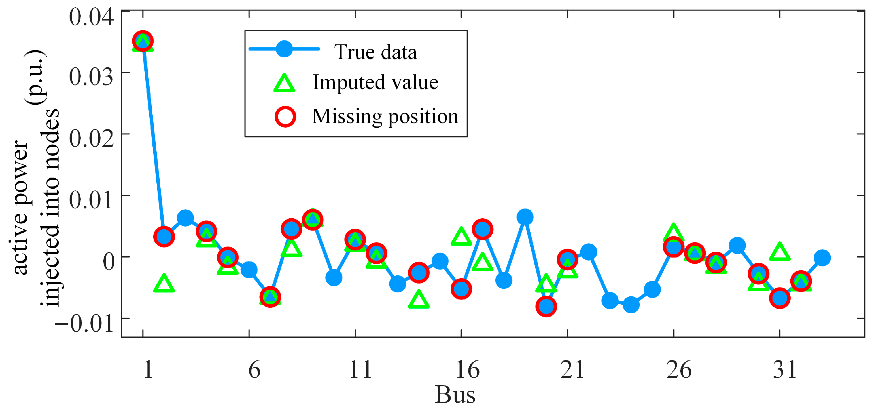
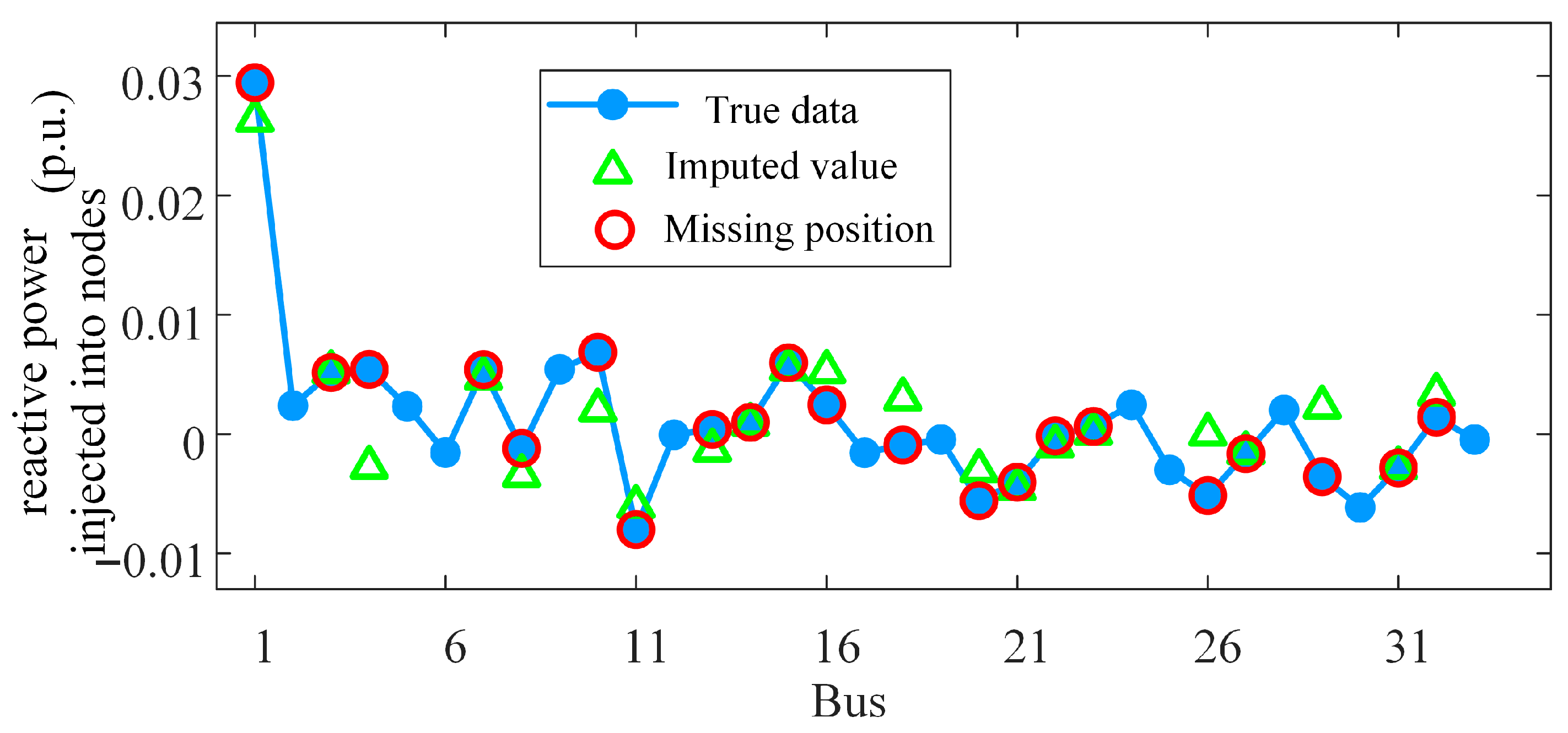
When designing the random missingness scenario, the experiment adopts a generation strategy that constrains the total amount of missingness and randomly assigns missing positions for the binary mask matrix B. Specifically, the total amount of missing data is controlled by a preset missingness rate (set to 10% in the experiments conducted in this paper), while the missing points are randomly distributed across the spatial and temporal dimensions to simulate real-world scenarios. A random set from the imputed matrix (Figure 8, Figure 9 and Figure 10) demonstrates the proposed method’s imputation effect.

In Figure 8, blue circles denote “true data”, green triangles “imputed values”, and red circles “missing positions”. The figure demonstrates the proposed method’s strong reconstruction capability for scattered missing points, with voltage magnitude imputation results highly consistent with the true curve and accurate restoration of sparse data regions. Figure 9 and Figure 10 present node active and reactive power injection imputations, respectively; despite short-term fluctuations in the original data at some missing positions, the model effectively captures changing trends, with imputed values matching the true data in value and shape.

5.2. Results of Continuous Missing Measurement Data Imputation

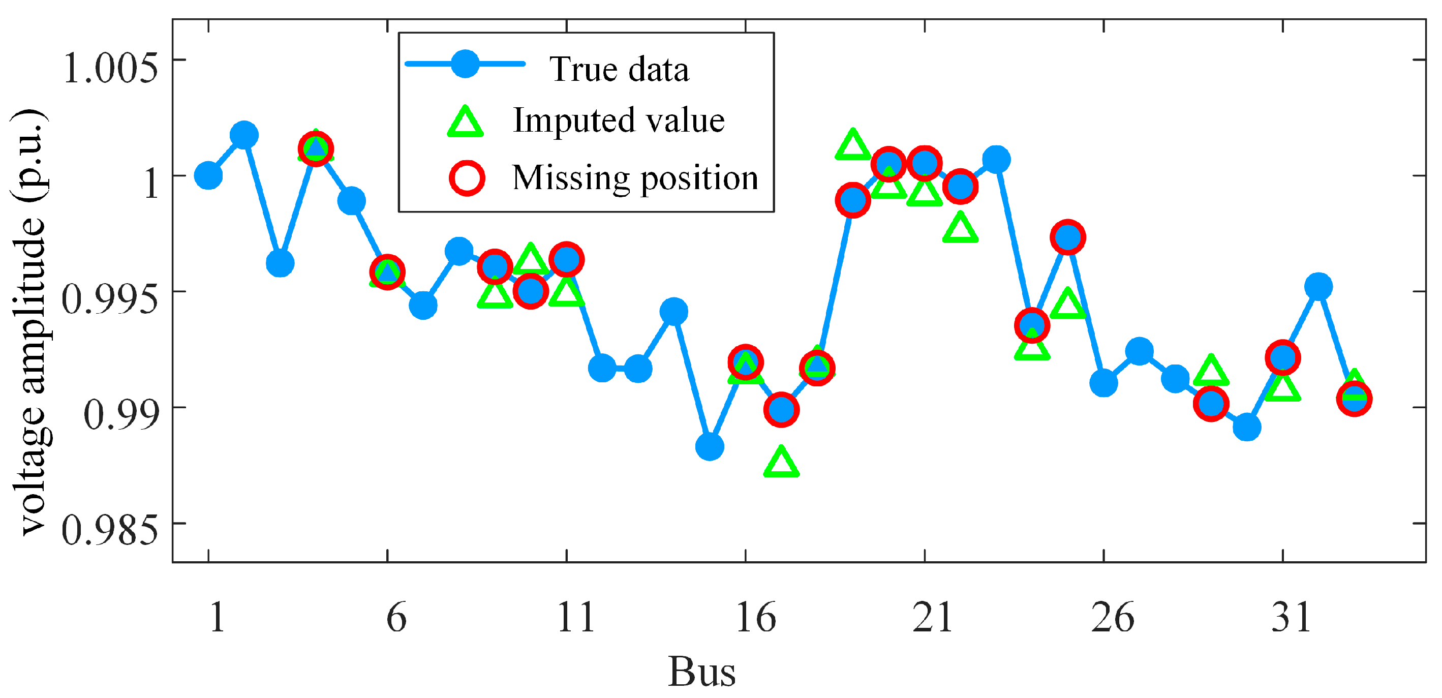
The continuous missing scenario was designed with seven consecutive days of missing measurement data, with true data, imputed values, and missing positions shown in Figure 11, Figure 12 and Figure 13.

Data reconstruction under the continuous missing scenario is more challenging due to concentrated and long-duration missing segments. Nevertheless, the proposed method still demonstrates strong temporal modeling capability: Figure 11 shows stable voltage imputation with minimal errors, while Figure 12 and Figure 13 maintain consistent overall trends despite slight deviations at some positions. This indicates the model possesses excellent generalization and reconstruction performance for long-range temporal dependencies.

5.3. Analysis of the Model Training Process

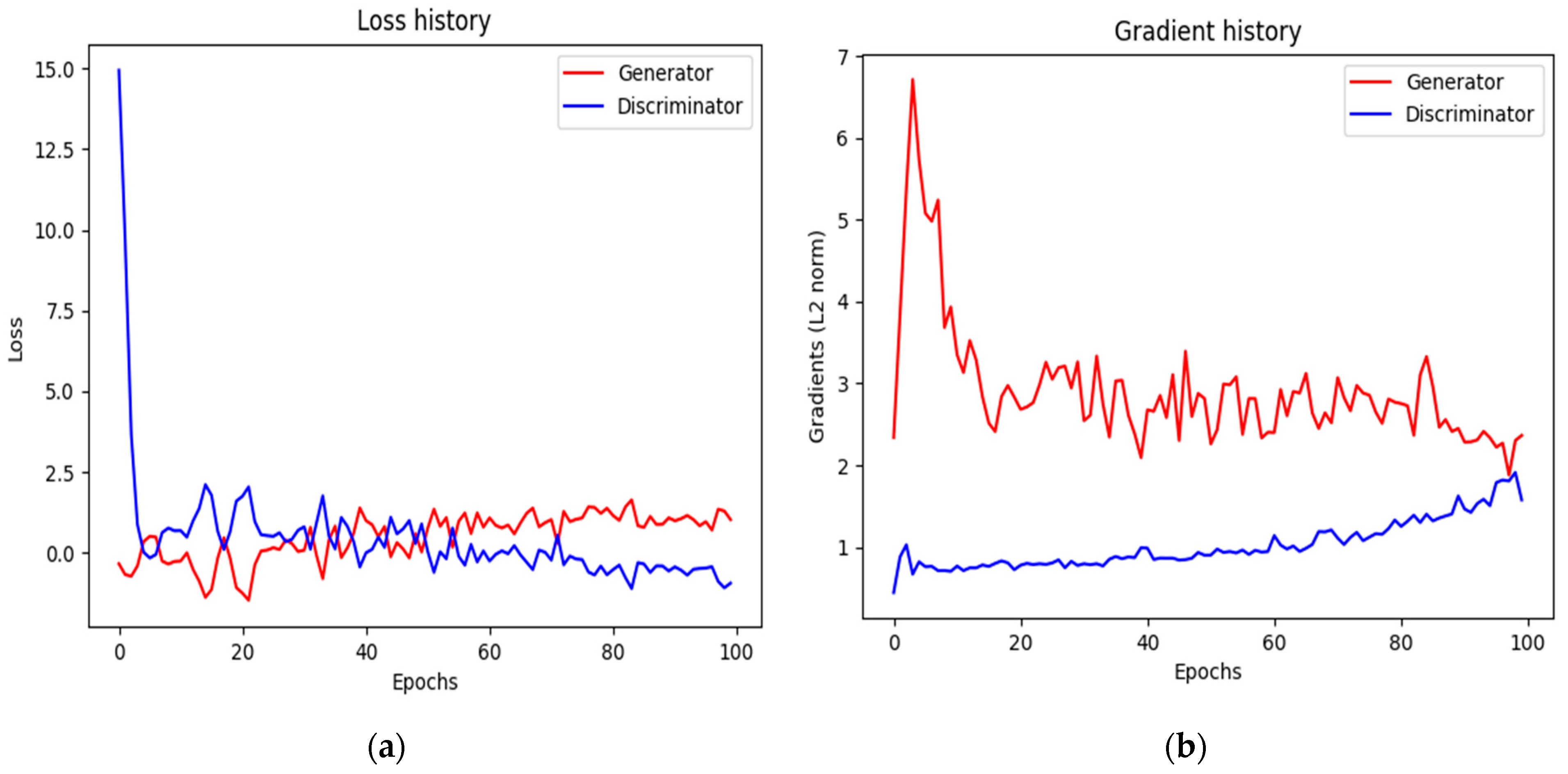
To demonstrate the convergence and stability of the proposed method during the training process, Figure 14 shows the loss and gradient histories of the generator and discriminator.

As shown in Figure 14a,b, the discriminator’s loss rapidly decreased and stabilized early in training, while the generator’s loss gradually converged to a dynamic balance with the discriminator, indicating the model achieved good convergence during adversarial training. The generator’s gradient fluctuated significantly initially but stabilized afterward; the discriminator’s gradient remained small and grew gently, demonstrating that the gradient penalty mechanism effectively suppressed gradient vanishing or exploding, thus ensuring model training stability.

5.4. Comparative Analysis

To verify the effectiveness and superiority of the TGAN-GP proposed in this paper for imputing missing measurement data in the distribution network, it is compared with other imputation methods. Under the two scenarios of “random missing” and “continuous missing”, the imputation error quantification metrics of the five methods are calculated, and the results are shown in

Table 1. Error Metrics under Random Missing Data.

Category	Metric	LSTM	Transformer	WGAN	WGAN-GP	Proposed Method
V 1	RMSE	0.00315	0.00074	0.00258	0.00311	0.00062
	MAE	0.00306	0.00088	0.00224	0.00247	0.00051
P 1	RMSE	0.00248	0.00246	0.00407	0.00473	0.00081
	MAE	0.00215	0.00191	0.00287	0.00362	0.00065
Q 1	RMSE	0.00465	0.00176	0.00376	0.00398	0.00082
	MAE	0.00403	0.00153	0.00324	0.00343	0.00076

¹ V is the voltage magnitude, P is the active power injected into the node, and Q is the reactive power injected into the node.

and

Table 2. Error Metrics under Continuous Missing Data.

Category	Metric	LSTM	Transformer	WGAN	WGAN-GP	Proposed Method
V	RMSE	0.00208	0.00176	0.00237	0.00279	0.00147
	MAE	0.00173	0.00153	0.00201	0.00215	0.00122
P	RMSE	0.00473	0.00537	0.00558	0.00389	0.00373
	MAE	0.00394	0.00482	0.00441	0.00329	0.00268
Q	RMSE	0.00412	0.00482	0.00471	0.00567	0.00314
	MAE	0.00335	0.00418	0.00399	0.00468	0.00226

.

As is evident from the two tables, the method proposed in this paper achieves better performance in both missing scenarios.

5.5. Comparison of Error Distributions

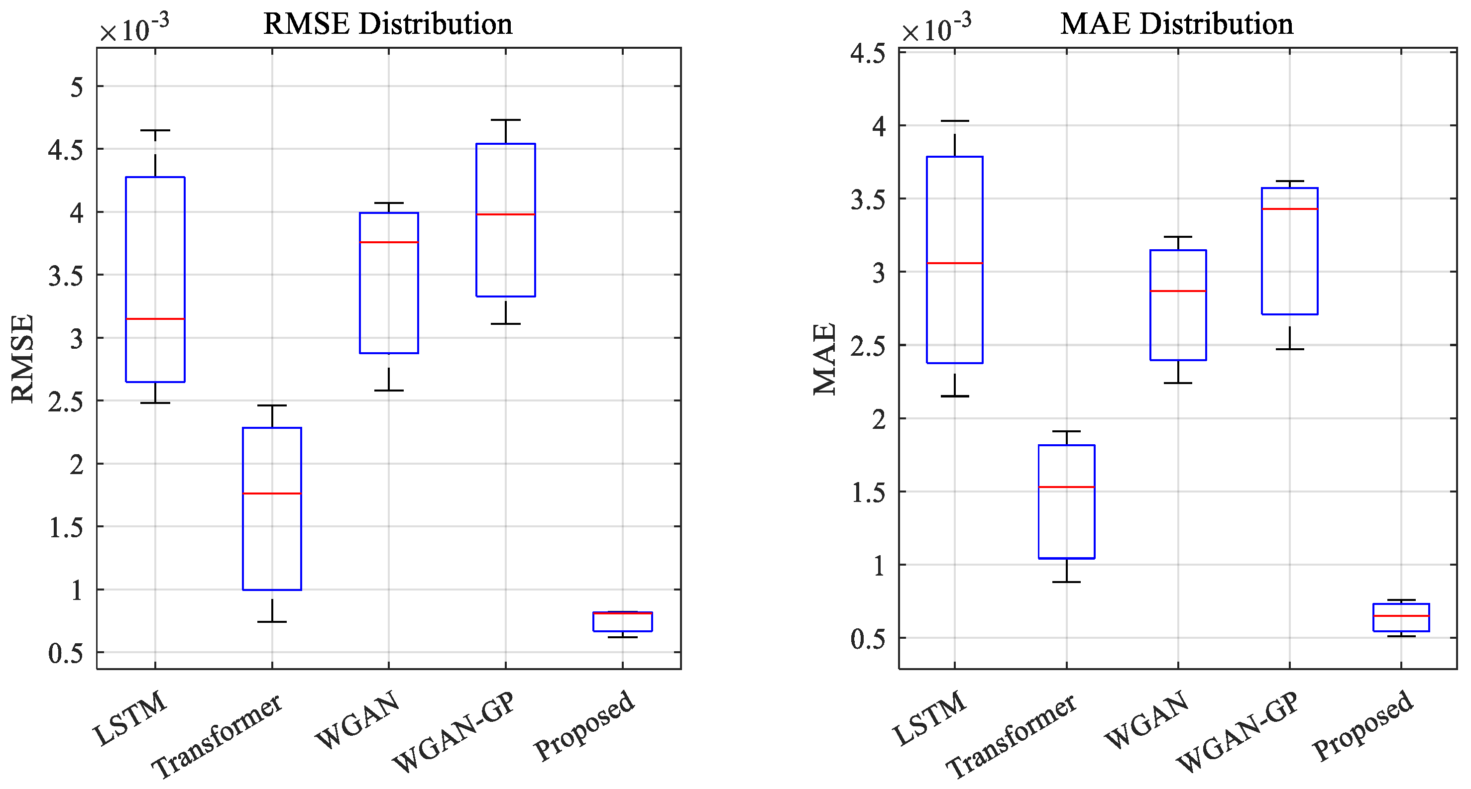
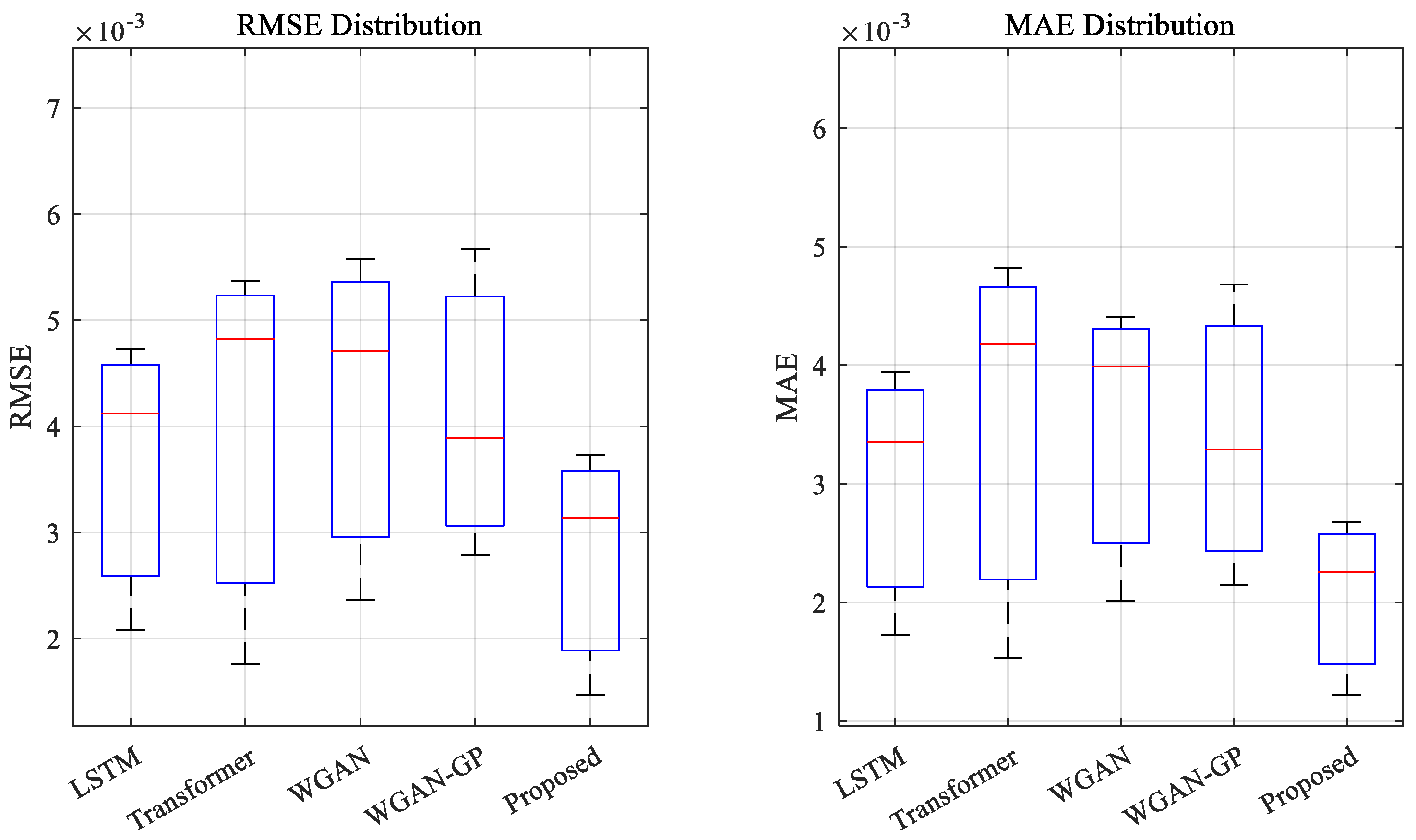
To enable a more comprehensive evaluation of each model’s performance in the imputation task, box plots are used to visualize the error fluctuations, central tendency, and outliers for different models, as shown in Figure 15 and Figure 16.

Figure 15 and Figure 16 show RMSE and MAE distribution boxplots for five models under the random and consecutive missing scenarios, respectively. Each boxplot illustrates the imputation error fluctuations (whisker range) and central tendency (median: red inner line) for voltage, active power, and reactive power. Under the random missing scenario (Figure 15), the proposed method has the smallest box range and median in both error distributions, indicating more stable and concentrated performance. In contrast, LSTM and WGAN exhibit larger fluctuations (wider boxes, longer whiskers). For the consecutive missing scenario (Figure 16), the proposed method maintains the most compact error distribution, while WGAN-GP and WGAN show relatively dispersed fluctuations. This further reflects the robustness of its architecture in handling complex missing patterns.

5.6. Ablation Study

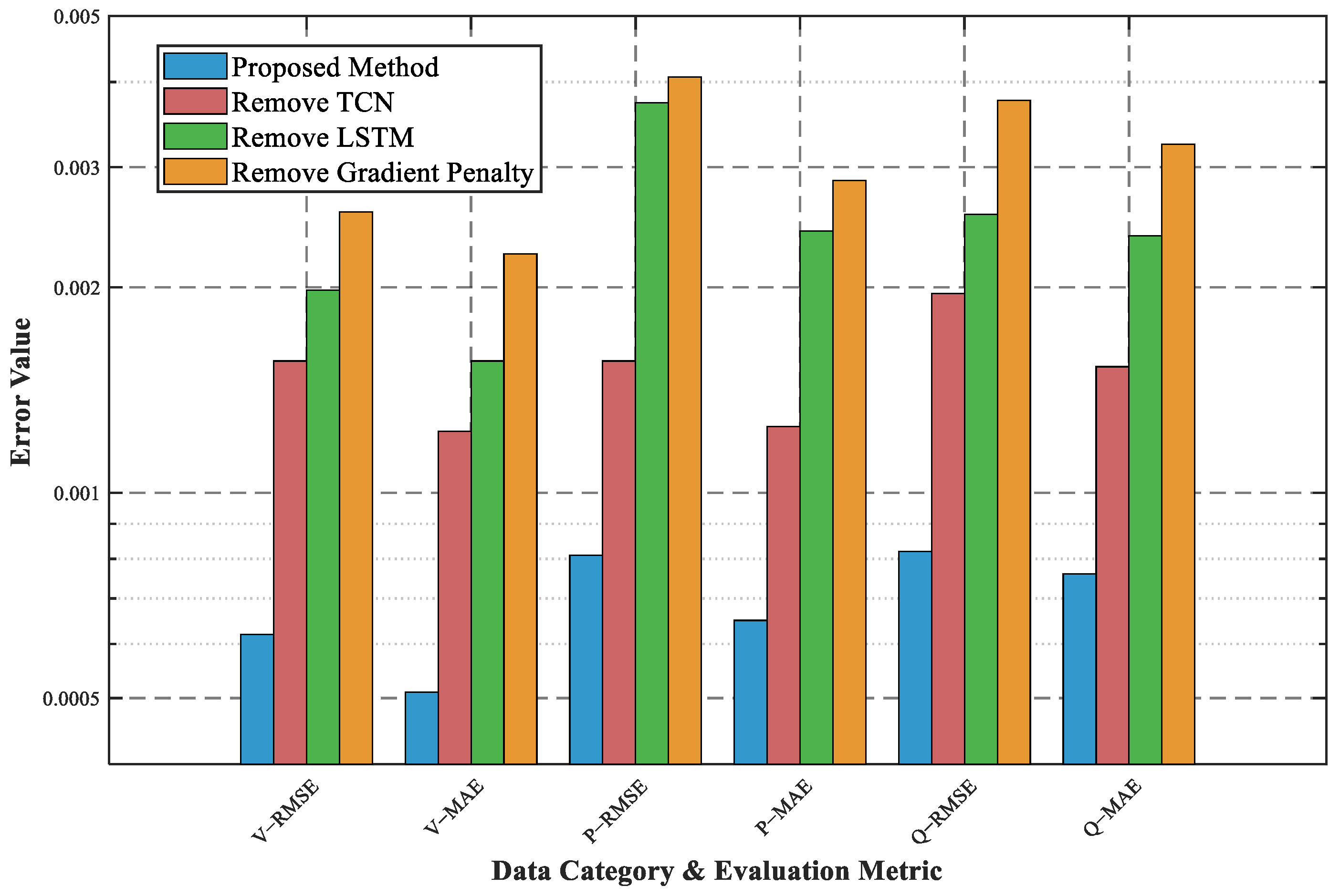
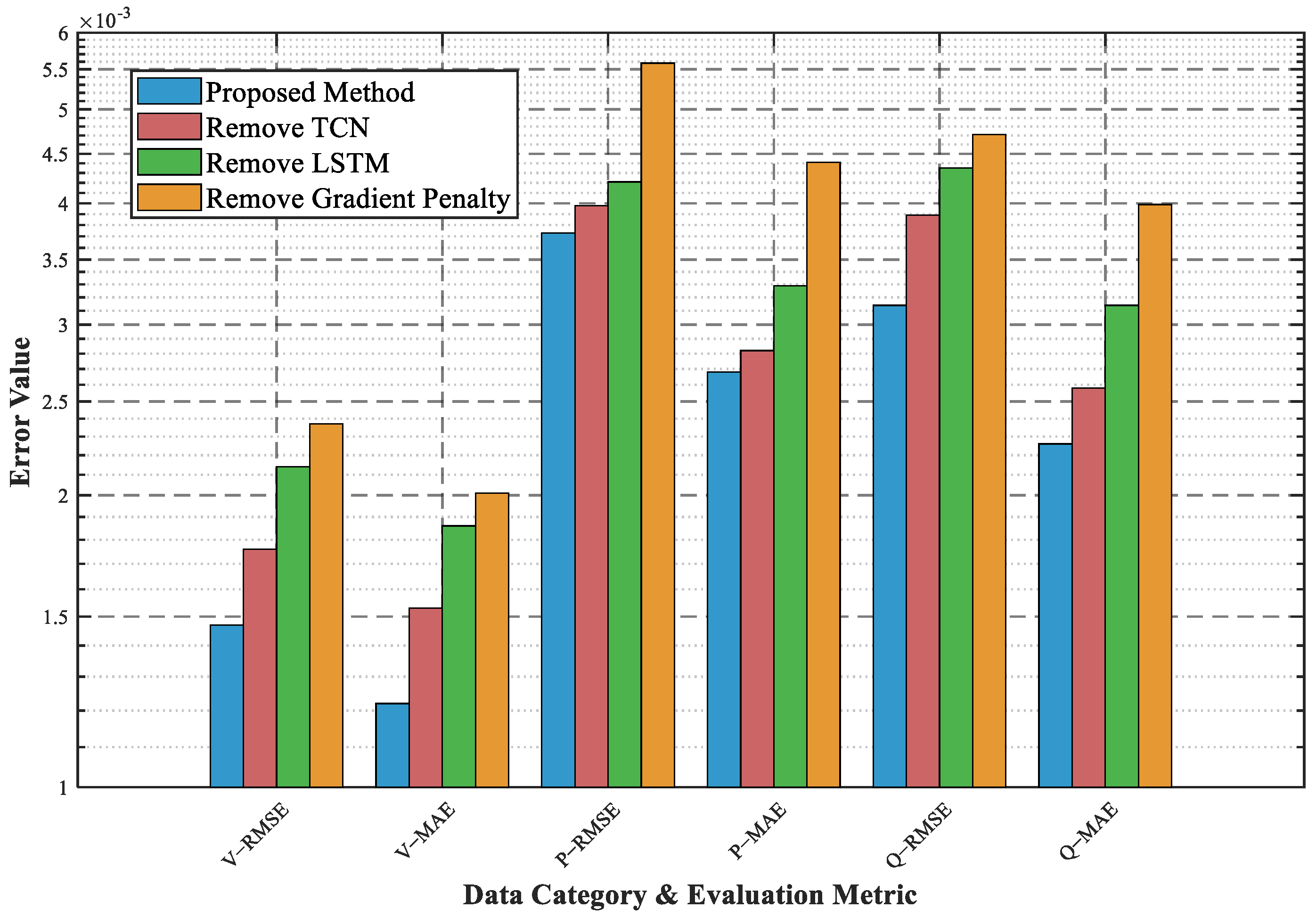
To verify the effectiveness of the proposed TGAN-GP method, three additional imputation variants are constructed by sequentially removing the TCN (generator), LSTM (discriminator), and gradient penalty term. These variants are used as comparative baselines, and the verification results are shown below.

Figure 17 and Figure 18 respectively illustrate the RMSE and MAE error distributions of the proposed model and its three ablation variants for three data types in two missing scenarios. Focusing on the random missing scenario, Figure 17 clearly shows that the errors of the original model are significantly lower than those of the ablation variants across all metrics. Targeting the continuous missing scenario, Figure 18 further verifies the original model’s optimal error performance, with a more pronounced increase in errors observed when LSTM or the gradient penalty term is removed. Together, these two figures intuitively demonstrate the necessity of each core component of TGAN-GP for improving imputation accuracy in missing data, while also reflecting the stability advantages of the original model under different missing scenarios.

6. Conclusions

This paper proposes a TGAN-GP-based missing data imputation method for distribution networks. By integrating WGAN-GP, TCN, and LSTM, it resolves the existing issues of unstable training and poor long-time series performance. Quantitative results on the IEEE 33-bus test system fully validate its significant improvements and core contributions.

Under the random missing scenario, compared to the LSTM network, the proposed method reduces the MAE by 83.3% and the RMSE by 82.9% for the node voltage magnitude imputation task. Compared to the Transformer, it decreases the MAE by 42.0% and the RMSE by 67.1%. Under the continuous missing scenario, the method reduces the MAE by 32.5% and the RMSE by 30.5% compared to LSTM and lowers the MAE by 46.0% and the RMSE by 34.9% compared to the Transformer. The gradient penalty mechanism ensures training stability, the TCN efficiently captures long-range temporal dependencies, and the LSTM discriminator enhances the evaluation of temporal rationality.

Future research will fuse GCN/GAT spatial features and TCN temporal dynamics to build a spatiotemporal framework for enhancing large-scale continuous missing data imputation and adopt lightweight technologies to balance TGAN-GP’s precision and real-time performance for better applicability to online distribution networks.

References

1. Li, Z.; Xia, Y.; Luo, Y.; Xiong, J. Research on the Development of a New Power System Under the “Dual Carbon” Goals. In Proceedings of the 2024 Boao New Power System International Forum—Power System and New Energy Technology Innovation Forum (NPSIF), Boao, China, 8–10 December 2024; IEEE: New York, NY, USA, 2024; pp. 758–762. [Google Scholar]
2. Bo, L.; Jiangang, L.; Jinhua, H.; Ruifeng, Z.; Kaiyan, P.; Wenjie, Z. A Massive Resource Power System Operation Supporting System Adapting to Dual Carbon Goals. In Proceedings of the 2023 International Conference on Power, Electrical Engineering, Electronics and Control (PEEEC), Athens, Greece, 25–27 September 2023; IEEE: New York, NY, USA, 2023; pp. 271–276. [Google Scholar]
3. Li, Y.; Geng, J.; Zhu, K.; Guo, X. Energy Internet-oriented Power trading Platform: Review and Prospect. In Proceedings of the 2022 7th Asia Conference on Power and Electrical Engineering (ACPEE), Online, 15–17 April 2022; IEEE: New York, NY, USA, 2023; pp. 482–487. [Google Scholar]
4. Miao, X.; Wu, Y.; Chen, L.; Gao, Y.; Yin, J. An Experimental Survey of Missing Data Imputation Algorithms. IEEE Trans. Knowl. Data Eng. 2023, 35, 6630–6650. [Google Scholar] [CrossRef]
5. Qiu, R.J.; Ding, J.Y.; Zhang, Z.K.; Han, P.P.; Wu, H.B.; Wu, J.Y. Pseudo-metric modelling of distribution network state estimation based on CNN-BiLSTM network and customized HGGA algorithm. Measurement 2024, 227, 114223. [Google Scholar] [CrossRef]
6. García, S.; Luengo, J.; Herrera, F. Dealing with Missing Values. In Data Preprocessing in Data Mining; García, S., Luengo, J., Herrera, F., Eds.; Springer International Publishing: Cham, Switzerland, 2015; pp. 59–105. [Google Scholar]
7. Kwak, S.; Kim, J. Statistical data preparation: Management of missing values and outliers. Korean J. Anesthesiol. 2017, 70, 407. [Google Scholar] [CrossRef] [PubMed]
8. Liu, J.; Cao, Y.; Li, Y.; Guo, Y.; Deng, W. Big Data Cleaning Based on Improved CLOF and Random Forest for Distribution Networks. CSEE J. Power Energy Syst. 2024, 10, 2528–2538. [Google Scholar] [CrossRef]
9. Jiang, Y.J.; He, T.T.; Yu, M.M.; Zhou, Y. Hybrid imputation of missing values using KNN on MEWMA-based adaptive process control. Qual. Technol. Quant. Manag. 2025, 1–21. [Google Scholar] [CrossRef]
10. Ma, J.; Cheng, J.C.P.; Jiang, F.; Chen, W.; Wang, M.; Zhai, C. A bi-directional missing data imputation scheme based on LSTM and transfer learning for building energy data. Energy Build. 2020, 216, 109941. [Google Scholar] [CrossRef]
11. Yu, X.M.; Wang, J.; Zhang, K.; Chen, Z.J.; Tong, M.; Sun, S.B.; Shen, J.P.; Zhang, L.; Wang, C.Y. Research on Missing Data Estimation Method for UPFC Submodules Based on Bayesian Multiple Imputation and Support Vector Machines. Energies 2025, 18, 2535. [Google Scholar] [CrossRef]
12. Yang, T.; Yang, Z.; Pen, H. Electricity Measurement Missing Data Recovery Method Based on Low-Rank Tensor Completion with Triangular Canonical Polyadic Decomposition. IEEE Trans. Instrum. Meas. 2025, 74, 9008713. [Google Scholar] [CrossRef]
13. Chen, X.; Liang, S.; Zhang, Z.; Zhao, F. A Novel Spatiotemporal Data Low-Rank Imputation Approach for Traffic Sensor Network. IEEE Internet Things J. 2022, 9, 20122–20135. [Google Scholar] [CrossRef]
14. Yu, Y.; Li, V.O.K.; Lam, J.C.K. Hierarchical Recovery of Missing Air Pollution Data via Improved Long-Short Term Context Encoder Network. IEEE Trans. Big Data 2023, 9, 93–105. [Google Scholar] [CrossRef]
15. Niako, N.; Melgarejo, J.D.; Maestre, G.E.; Vatcheva, K.P. Effects of missing data imputation methods on univariate blood pressure time series data analysis and forecasting with ARIMA and LSTM. BMC Med. Res. Methodol. 2024, 24, 320. [Google Scholar] [CrossRef] [PubMed]
16. Goodfellow, I.; Pouget-Abadie, J.; Mirza, M.; Xu, B.; Warde-Farley, D.; Ozair, S.; Courville, A.; Bengio, Y. Generative Adversarial Networks. arXiv 2014, arXiv:1406.2661. [Google Scholar] [CrossRef]
17. Kim, J.; Li, Y.; Shin, B.S. 3D-DGGAN: A Data-Guided Generative Adversarial Network for High Fidelity in Medical Image Generation. IEEE J. Biomed. Health Inform. 2024, 28, 2904–2915. [Google Scholar] [CrossRef]
18. Alonso-Monsalve, S.; Whitehead, L.H. Image-Based Model Parameter Optimization Using Model-Assisted Generative Adversarial Networks. IEEE Trans. Neural Netw. Learn. Syst. 2020, 31, 5645–5650. [Google Scholar] [CrossRef] [PubMed]
19. Jiang, N.N.; Zhao, W.B.; Wang, H.; Luo, H.Q.; Chen, Z.Z.; Zhu, J.B. Lightweight Super-Resolution Generative Adversarial Network for SAR Images. Remote Sens. 2024, 16, 1788. [Google Scholar] [CrossRef]
20. Chang, Y.H.; Chung, P.H.; Chai, Y.H.; Lin, H.W. Color Face Image Generation with Improved Generative Adversarial Networks. Electronics 2024, 13, 1205. [Google Scholar] [CrossRef]
21. Lou, X.P.; Wang, L.H. QuanFlex-GAN: A flexible algorithm for image generation via quantum generative modeling. Quantum Mach. Intell. 2025, 7, 87. [Google Scholar] [CrossRef]
22. Zhang, W.; Luo, Y.; Zhang, Y.; Srinivasan, D. SolarGAN: Multivariate Solar Data Imputation Using Generative Adversarial Network. IEEE Trans. Sustain. Energy 2021, 12, 743–746. [Google Scholar] [CrossRef]
23. Feng, G.; Lao, K.W. Wasserstein Adversarial Learning for Identification of Power Quality Disturbances with Incomplete Data. IEEE Trans. Ind. Inform. 2023, 19, 10401–10411. [Google Scholar] [CrossRef]
24. Li, H.Y.; Pei, K.X.; Sun, W.Q. Dynamic State Estimation for Power System Based on the Measurement Data Reconstructed by RGAN. IEEE Access 2021, 9, 92578–92585. [Google Scholar] [CrossRef]
25. Wang, C.G.; Cao, Y.; Zhang, S.; Ling, T. A Reconstruction Method for Missing Data in Power System Measurement Based on LSGAN. Front. Energy Res. 2021, 9, 651807. [Google Scholar] [CrossRef]
26. Boronuosi, F.; Azad, S.; Ameli, M.T.; Shadi, M.R. Dynamic security assessment of power systems using a deep learning and GAIN-based approach for addressing missing data. Results Eng. 2025, 27, 106585. [Google Scholar] [CrossRef]
27. Li, J.B.; Chen, Z.Q.; Cheng, L.; Liu, X.F. Energy data generation with Wasserstein Deep Convolutional Generative Adversarial Networks. Energy 2022, 257, 124694. [Google Scholar] [CrossRef]
28. Wang, S.X.; Chen, H.W.; Pan, Z.X.; Wang, J.M. A Reconstruction Method for Missing Data in Power System Measurement Using an Improved Generative Adversarial Network. Proc. CSEE 2019, 39, 56–64+320. [Google Scholar] [CrossRef]
29. Ruan, J.; Fan, G.; Zhu, Y.; Liang, G.; Zhao, J.; Wen, F.; Dong, Z.Y. Super-Resolution Perception Assisted Spatiotemporal Graph Deep Learning Against False Data Injection Attacks in Smart Grid. IEEE Trans. Smart Grid 2023, 14, 4035–4046. [Google Scholar] [CrossRef]
30. Donti, P.L.; Liu, Y.J.; Schmitt, A.J.; Bernstein, A.; Yang, R.; Zhang, Y.C. Matrix Completion for Low-Observability Voltage Estimation. IEEE Trans. Smart Grid 2020, 11, 2520–2530. [Google Scholar] [CrossRef]
31. Pachika, S.; Reddy, A.B.; Pachika, B.; Karnam, A. Generative Adversarial Networks: Overview. In Proceedings of the Fifth International Conference on Computer and Communication Technologies; Devi, B.R., Kumar, K., Raju, M., Raju, K.S., Sellathurai, M., Eds.; Springer Nature: Singapore, 2024; pp. 319–328. [Google Scholar]
32. Zhang, Y.Q.; Zhang, R.T.; Zhao, B.T. A systematic review of generative adversarial imputation network in missing data imputation. Neural Comput. Appl. 2023, 35, 19685–19705. [Google Scholar] [CrossRef]
33. Han, D.; Bai, H.K.; Wang, Y.Y.; Wang, S.Q.; Zhang, J.; Liu, Y. An Improved TCN Considering Data Augmentation in Enabling Load Classification. J. Circuits Syst. Comput. 2022, 31, 2250284. [Google Scholar] [CrossRef]
34. Santhi, P.; Bhaskaran, V.M. Improving the Efficiency of Image Clustering using Modified Non Euclidean Distance Measures in Data Mining. Int. J. Comput. Commun. Control 2014, 9, 56–61. [Google Scholar]
35. Dolatabadi, S.H.; Ghorbanian, M.; Siano, P.; Hatziargyriou, N.D. An Enhanced IEEE 33 Bus Benchmark Test System for Distribution System Studies. IEEE Trans. Power Syst. 2021, 36, 2565–2572. [Google Scholar] [CrossRef]
36. Xie, X.; Lei, Y.; Xiang, C.Y.; Li, Y.X.; Liu, L.J. An Enhanced Generative Adversarial Imputation Network with Unsupervised Learning for Random Missing Data Imputation of All Sensors. Struct. Control Health Monit. 2025, 2025, 8419570. [Google Scholar] [CrossRef]
Figure 1. Schematic Diagram of Missing Types for Distribution Network Measurement Data (a) Random missing scenario; (b) Continuous missing scenario.
Energies 19 00030 g001
Figure 2. Architecture Diagram of Generative Adversarial Network.
Energies 19 00030 g002
Figure 3. Schematic Diagram of Causal Dilated Convolution in TCN.
Energies 19 00030 g003
Figure 4. Schematic Diagram of Residual Block in TCN.
Energies 19 00030 g004
Figure 5. Schematic Diagram of LSTM Structure for Discriminator.
Energies 19 00030 g005
Figure 6. Training Process Diagram of TGAN-GP Model.
Energies 19 00030 g006
Figure 7. Topology Diagram of the IEEE 33-bus Distribution Network Test System.
Energies 19 00030 g007
Figure 8. Imputation Results of Voltage Magnitude Under the Random Missing Scenario.
Energies 19 00030 g008
Figure 9. Imputation Results of Node Active Power Injection Under the Random Missing Scenario.
Energies 19 00030 g009
Figure 10. Imputation Results of Node Reactive Power Injection Under the Random Missing Scenario.
Energies 19 00030 g010
Figure 11. Imputation Results of Voltage Magnitude Under the Continuous Missing Scenario.
Energies 19 00030 g011
Figure 12. Results of Node Active Power Injection Under the Continuous Missing Scenario.
Energies 19 00030 g012
Figure 13. Results of Node Reactive Power Injection Under the Continuous Missing Scenario.
Energies 19 00030 g013
Figure 14. Training Convergence and Stability Curves of the TGAN-GP Model. (a) Loss variation curves of generator and discriminator in training; (b) Gradient fluctuation curves of generator and discriminator in training.
Energies 19 00030 g014
Figure 15. Boxplots of RMSE and MAE distributions across different models under the random missing scenario.
Energies 19 00030 g015
Figure 16. Boxplots of RMSE and MAE distributions across different models under the consecutive missing scenario.
Energies 19 00030 g016
Figure 17. Comparison distribution of RMSE/MAE among ablation variants under the random missing scenario.
Energies 19 00030 g017
Figure 18. Comparison distribution of RMSE/MAE among ablation variants under the continuous missing scenario.
Energies 19 00030 g018