Data-Driven Reliability Assessment of PV Inverters Using SCADA Measurements

Abstract

This paper presents a case study framework for the operational reliability monitoring of a grid-connected photovoltaic (PV) inverter using SCADA measurements collected during February–April 2025. The workflow combines correlation-based drift analysis, probabilistic outputs from established machine learning models (XGBoost and LSTM), and temporal consistency modeled through a hidden Markov model (HMM). The resulting evidence is summarized into two interpretable composite indicators: a Health Index (HI), intended to capture short-term deviations, and a Reliability Score (RS), intended to provide a smoother reliability-oriented summary over time. A time-aware evaluation protocol is employed to reduce temporal leakage and to assess predictive utility under rare-event conditions, complemented by baseline comparisons and sensitivity checks for key thresholds and modeling settings. Within the analyzed dataset, the results suggest that HI is responsive to transient disturbances, while RS supports trend monitoring and maintenance prioritization by consolidating multiple weak signals into a consistent operational view. The proposed indicators are positioned as data-driven risk summaries for decision support rather than direct physical measures of deviation patterns. Generalization to other inverters and sites requires further validation on longer horizons and with additional operational/maintenance records.

1. Introduction

Photovoltaic (PV) systems have become a key component of the global energy transition, providing sustainable and environmentally friendly electricity. Among the many elements that make up a PV system, the inverter plays a key role as the interface between the direct current (DC) generator and the alternating current (AC) grid. As the “heart” of the system, it is responsible for conversion, grid synchronization, and the implementation of safety and monitoring functions. Due to their high complexity and operation under highly dynamic load conditions, inverters are also the most vulnerable components, statistically ranking among the leading sources of failure in PV systems [1,2]. The reliability of PV inverters is crucial for the overall efficiency and economic viability of solar power plants. Inverter failures lead to generation interruptions, financial losses, and unplanned repair costs. According to reports from PV park operations, the share of inverter-related failures can reach 60% of all recorded system failures [3]. This poses serious challenges for operators and maintenance, who must look for new approaches for predictive diagnostics and assessment of the health of the devices.

Traditional methods for monitoring and maintaining inverters are mainly reactive, based on alarm registration and subsequent intervention by service personnel. This approach is insufficient in the conditions of modern PV systems, where continuous operation and minimizing downtime are critically important. In recent years, attention has been focused on the concept of predictive maintenance, which uses available data and analytical methods for early detection of deviation patterns and prevention of failures.

SCADA systems play a central role in this process. They provide continuous collection and archiving of inverter operating parameters: DC voltages and currents, AC voltages and currents, frequency, power element temperature, conversion efficiency, output active and reactive power, as well as fault and alarm statuses. The collected data allows not only current operation, but also long-term analysis for reliability assessment. However, the huge volume of data and complex dependencies between parameters require the use of advanced analytical approaches that go beyond classical statistics. Over the past decade, artificial intelligence (AI) and machine learning (ML) methods have shown enormous potential for diagnostics and forecasting in the energy industry. Algorithms such as XGBoost and random forest (RF) provide high accuracy in classifying states and identifying the most relevant factors affecting reliability. On the other hand, recurrent neural networks and their derivatives (LSTM, GRU) are suitable for predicting time series and dynamics of processes such as load, temperature, and efficiency of inverters [4,5]. An additional tool is HMM, which allows the modeling of transitions between different states of the inverter: normal, degraded, and pre-failure.

In the literature, there are already works on assessing the reliability of PV inverters using statistical methods, such as Weibull distribution analysis and mean time between failure (MTBF) estimation [6]. However, most of them rely on historical failure data, which are often limited, incomplete, or difficult to access. There is a lack of a unified approach that uses real-time data from SCADA systems to build a dynamic reliability index that can be used both for monitoring and for predicting potential failures.

In view of this, the present work proposes an integrated framework for assessing the reliability of PV inverters, which combines the following:

• Correlation analysis of SCADA parameters for anomaly detection and “correlation drift”;
• XGBoost model for assessing the significance of features and classifying states;
• LSTM network for predicting the probability of failure over time;
• HMM for modeling the transitions between healthy, degraded, and failed states;
• Construction of HI and RS, which collectively reflect the health status of the inverter.

The proposed workflow integrates correlation drift, supervised ML probabilities, and HMM-based temporal consistency into interpretable composite indicators (HI/RS) for SCADA-only monitoring. It is presented as a case study demonstration, with broader validation left for future multi-inverter studies.

2. Literature Review

2.1. Classical Statistical Approaches to Reliability

The initial research on the reliability of PV systems relied on classical statistical models. The most widely used is the Weibull distribution analysis, which allows us to estimate the degradation rate and the mean time to failure of inverters and other components [7]. Such models are valuable for life cycle assessment, but they assume stationarity and require the availability of rich historical failure data.

In [8], statistical methods are integrated with ML models for the analysis of PV inverters using SCADA data. They show that combining classical reliability metrics (MTBF, Weibull β and η) with ML classifiers can significantly improve the accuracy of predictions. This highlights the potential for synergy between traditional and modern approaches.

2.2. SCADA Systems as a Key Data Source

With the increasing implementation of SCADA platforms in PV plants, these systems are becoming the main source of data for reliability analyses. SCADA provides detailed real-time measurements: voltages, currents, frequency, temperature, alarms, and faults.

In [9], they show how SCADA data can be used to build a predictive maintenance system that detects early signs of failure using ML algorithms. This is an important step from reactive to proactive maintenance.

In [10], they propose an IoT-based architecture for SCADA, including edge and cloud components, microservices, and blockchain for security. Similar developments show that SCADA data can be the basis for global reliability management systems.

2.3. Machine Learning for PV Inverter Diagnostics

In recent years, ML has established itself as a leading tool for fault detection and predictive maintenance. In [11], they developed a big-data predictive maintenance system using two ML modules to predict the overall probability of failure and to classify specific types of faults. They showed that failures can be predicted up to 7 days in advance with over 90% accuracy. In [12], they compared multiple ML algorithms on 2.2 million SCADA records and found that bagged tree models are the most effective for diagnostics, with an accuracy of 92.2%. In [13], they proposed an IoT-AI system where ML models not only diagnose problems but also initiate automatic actions (e.g., panel cleaning). These examples show that ML can be applied to both passive diagnostics and active maintenance.

2.4. Degradation Mechanisms and Reliability Through Probabilistic Models

Along with ML, stochastic models remain an important tool [14]. Here, unsupervised ML and HMM are used for failure mechanisms in PV inverters, modeling the transitions between healthy, degraded, and failed states. This approach allows the identification of the probabilities of future transitions, which is a valuable tool for predictive maintenance. The proposed approach approaches this direction by combining HMM with supervised ML (XGBoost, LSTM) and correlation analysis. This provides a more comprehensive framework—classification, prediction, and stochastic modeling.

2.5. Review Studies and Industry Trends

Several review articles outline global trends. In [15], reliability methods in grid-connected PV systems are analyzed, comparing classical statistical and ML approaches. In [16], ML in predictive maintenance, including PV, is reviewed and data quality and interpretability issues are discussed. In [17], reliability methods are reviewed, emphasizing the need for integrated approaches that combine classical reliability analysis with data-driven models. These studies suggest that PV system reliability is a multidisciplinary problem requiring engineering, and statistical and ML solutions simultaneously.

2.6. Limitations and Gaps in the Literature

Despite significant progress, the existing approaches have limitations, such as noise and incompleteness in SCADA data. ML models are often sensitive to missing or anomalous values. Rare events: Failures are few in number, leading to serious imbalance in classes. Interpretability: Deep neural networks are difficult to explain in engineering practice. Generalization: Models trained for a specific park or manufacturer do not always adapt to other conditions. These gaps determine the need for hybrid frameworks (such as the proposed HI + RS) that combine the advantages of different methods.

2.7. Summary

The literature review shows the evolution of reliability research, from classic MTBF/Weibull analyses to AI-based, data-driven approaches using SCADA data. However, few studies offer an integrated methodology, including correlation analysis for early diagnosis, combining ML (XGBoost, LSTM) with HMM, defining aggregated indicators such as HI and RS.

The proposed framework fills this gap by creating a comprehensive tool for monitoring, diagnosing, and predicting the reliability of PV inverters.

3. Data and Methodology

The proposed methodology is based on an integrated analytical approach that combines statistical analysis, machine learning methods (XGBoost, LSTM), stochastic modeling (HMM), and aggregated indicators (HI/RS) for assessing the reliability of PV inverters [18,19]. The data are extracted from SCADA systems that record basic electrical and temperature parameters in real time, as well as error signals [20].

Let ${\left\{\left(x_t,y_t\right)\right\}}_{t=1}^T$ be a time-discretized set of SCADA observations with a step Δt = 5 min, where $x_t\in R^d$ is a vector of features (electrical, thermal, and aggregated quantities), and $y_t\in \left\{0,1\right\}$ indicates an error/incident (1) or normal operation (0). The process includes the following main stages:

• Collection and preprocessing of SCADA data;
• Feature engineering and correlation analysis;
• Instantaneous probability of an incident $p_t=P\left(y_t={\displaystyle \raisebox{1ex}{$1$}\!\left/ \!\raisebox{-1ex}{$F_t$}\right.}\right)$;
• Classification and prediction using ML models;
• Stochastic modeling of transitions between hidden states using HMM $S_t\in \left\{\mathrm{Normal}, \mathrm{Anomaly}, \mathrm{Error}\right\}$;
• Construction of aggregated indicators—HI $H{I}_t [0,1]$ and RS $R{S}_t [0,1]$.

The data are extracted from a SCADA system with a recording frequency of 5 min. The parameters used include the following: DC side: voltages (Udc), currents (Idc), output DC power (Pdc); AC side: voltages (Uac1, Uac2, Uac3), currents (Iac1, Iac2, Iac3), frequency (fac), output active power (Pac); temperature: Temp (degC) of the power elements; conversion efficiency: InvEff (%); status signals: errors (error), alarms.

The data preprocessing includes the following sequence. Remove missing and incorrect values and apply consistent mask-based imputation rules to preserve time continuity [21]. For $x^{\left(j\right)}$ a feature, we define a mask $m_t^{\left(j\right)}\in \left\{0,1\right\}$ and impute ${\tilde{x}}^{\left(j\right)}=\varphi \left(x_t^{\left(j\right)}\right)$. We normalize the parameters by using the following MinMaxScaler [22]:

$${\hat{x}}_t^{\left(j\right)}={\displaystyle \frac{{\tilde{x}}_t^{\left(j\right)}-\min \left({\tilde{x}}^{(j)}\right)}{\max \left({\tilde{x}}^{(j)}\right)-\min \left({\tilde{x}}^{(j)}\right)}}\in [0,1]$$

(1)

where $x_t^{(j)}$ is a raw measured quantity (e.g., voltage, current, temperature) for record t; $x^{\min }, x^{\max }$ are the minimum/maximum in the training window; ${\tilde{x}}_t^{(n)}\in [0,1]$ is the normalized unitless value. All features are scaled to [0, 1] to support ML training to a general problem for ML processing.

The extraction of temporal characteristics (time of day, sine/cosine transformation for cyclicity) [23,24] through time encodings is conducted by using the following equations:

$$\begin{array}{l}{h}_t=hour+{\displaystyle \frac{\min }{60}},\\ {\sin }_t=\sin \left(2\pi {\displaystyle \raisebox{1ex}{$h_t$}\!\left/ \!\raisebox{-1ex}{$24$}\right.}\right),\\ {\cos }_t=\cos \left(2\pi {\displaystyle \raisebox{1ex}{$h_t$}\!\left/ \!\raisebox{-1ex}{$24$}\right.}\right).\end{array}$$

(2)

where h_t is the hour component (hour + minutes/60); sin(2πh_t/24) and cos(2πh_t/24) are cyclic projections in [−1, 1], without units, that encode the diurnal cycle and prevent a break at midnight.

For feature engineering and correlation analysis, let S be a set of selected features. We measure the Pearson correlation as follows:

$$R_{ij}=corr\left(x^{(i)},x^{(j)}\right), R\in {[-1,1]}^{\left|S\right|}$$

(3)

where x_ij is the correlation coefficient between features i and j (−1 ≤ x_ij ≤ 1). It is used for feature selection and dependency tracking.

For a base matrix $R^{(0)}$ (defined over a reference baseline window) and a current rolling-estimated $R_t^{(\omega )}$ window $\omega$, we define drift as follows:

$$D_t={‖R_t^{(\omega )}-R^{(0)}‖}_F$$

(4)

where $R^{(0)}$ is a base correlation matrix; $R_t^{(\omega )}$ is a current sliding window matrix; ${‖R_t^{(\omega )}-R^{(0)}‖}_F$ is the Frobenius norm. Exponential smoothing exponentially weighted moving average and cumulative SUM for changes are added [25]. D_t is entered as a risk indicator in HI_t.

The correlations are classified by strength (weak, moderate, strong) and are used to select input features for ML models.

3.1. Classification and Prediction Using ML Models

3.1.1. XGBoost Classifier

We train a gradient boosted tree on independent observations $\left(x_t,y_t\right)$ with attention to time leaks, such as block splitting [18,26]. The model optimizes logistic loss through the following equation:

$$L_{XGB}=-{\displaystyle \sum _t\left[y_t\log p_t^{XGB}+\left(1-y_t\right)\log \left(1-p_t^{XGB}\right)+\mathrm{\Omega }(\tau )\right]}$$

(5)

where y_t ∈ {0, 1} is the label (error/norm); $p_t=P\left(y_t={\displaystyle \raisebox{1ex}{$1$}\!\left/ \!\raisebox{-1ex}{$x_t$}\right.}\right)$ is the probability of the model; $\mathrm{\Omega }(\tau )$ is the regularization of the trees (complexity control). It is optimized for two-class diagnostics.

We use gain/cover/frequency statistics and SHAP-based interpretation to support feature relevance assessment and to derive normalized weights for the composite indicators [18].

3.1.2. LSTM Model

We form sequences with window L: $X_{\tau }=\left[x_{\tau -L+1},\dots ,x_{\tau }\right]$ and target $y_{\tau +\delta }$ at horizon δ [19,27]. Here, L denotes the temporal lookback window length (number of past time steps), while the window is advanced with a unit stride. The index τ corresponds to the last time step of the input sequence, and δ defines the prediction horizon between the input window and the target. LSTM is implemented as follows:

$$p_{\tau +\delta }^{LSTM}=\sigma \left(f_{\theta }(X_{\tau })\right)$$

(6)

where σ is sigmoid; f_θ is a parameterized recurrent network. Loss (binary cross-entropy) with class weights for imbalance [28,29,30,31,32,33,34] is calculated as follows:

$$L_{LSTM}=-{\displaystyle \sum _{\tau }\left[{\omega }_{1}y\log p+{\omega }_0\left(1-y\right)\log \left(1-p\right)\right]}, {\displaystyle \frac{{\omega }_1}{{\omega }_0}}\approx {\displaystyle \frac{N_0}{N_1}}$$

(7)

where ${\omega }_{y_t}$ are class weights for imbalance (higher for the rare class “error”); the remaining quantities are as denoted in Equation (5).

3.1.3. Random Forest for Incident Typology

We train random forest (RF) only for post hoc typification of incidents (temperature, frequency, voltage, efficiency, etc.) and for validating the interpretability of feature importance, in parallel with XGBoost/SHAP. The module does not participate in the calculation of RS, which is formed by ${\hat{\pi }}^{XGB},{\hat{\pi }}^{LSTM},$ and HMM consistency. Thus, RF performs two functions: operational classification of incident type for clearer alarms to maintenance and cross-validation of the dominant factors identified by XGBoost (efficiency, energy, temperature, etc.), without changing HI/RS.

Multi-label/multi-class setting for $c\in \left\{Temp,Freq,Volt,Eff,\dots \right\}$. We train RF [35,36] with class weights. A probability vector ${\hat{\pi }}_t^{RF}$ supports the analysis and builds on HI.

3.2. Stochastic Modeling Using HMM

To model the transitions between states of the inverter, HMM with three states is used [28,29] as follows:

• S0—Healthy state (normal operation);
• S1—Anomaly (operational deviations);
• S2—Failure (incident or failure).

We define a hidden process $\left\{S_t\right\}$ with states:

$$S_t=\left\{S_0=\mathrm{Normal}, S_1=\mathrm{Anomaly}, S_2=\mathrm{Error}\right\}$$

(8)

The parameters $\lambda =\left(\pi ,A,B\right)$ include initial probabilities $\pi =\left[{\pi }_0,{\pi }_1,{\pi }_2\right],{\displaystyle {\sum }_i{\pi }_i=1}$, transition matrix $A=\left[a_{ij}\right], a_{ij}=P\left(S_t=j|S_{t-1}=i\right)$, and emission density for observations z_t (e.g., [InvEff, Temp, Δf, ΔV, Dt]). We choose Gaussian mixtures and a multinomial model after discretization.

We estimate λ with a Baum–Welch filter and Viterbi also gives $P\left(S_t=i|z_{1:t}\right)$ the most probable trajectory.

If we treat S2 as absorbing and analyze the hitting time to S2, the expected time to failure from normal is as follows:

$$MTBF\approx E\left[{\tau }_{S_2}|S_0\right], {\tau }_{S_2}=\inf \left\{t\ge 0:S_t=S_2\right\}$$

(9)

where when treating S₂ as an absorbing state, Q is a submatrix of transitions between temporary states (e.g., S₀, S₁), and the expected times to absorption are t = N₁. The component $t_{S_0}$ is the expected time to failure, starting from normal.

In the present study, this absorbing-state formulation is not applied to the analyzed data and is included solely as a conceptual extension for catastrophic faults or longer-term studies.

In discrete time, for HMM chains with transient states, a fundamental matrix $N={\left(I-Q\right)}^{-1}$ is used, where $Q$ is a submatrix of the transient states, used to derive the expected times.

Let $x_t=\left\{f_t,U_t^{1,2,3},T_t,{\eta }_t\right\}$ be the vector of observations at time t. We discretize it into indicators compatible with power quality standards and good monitoring practices: the frequency is assumed to be normal at 49.5  ≤  f_t ≤ 50.5 Hz, for an anomaly in single disturbances in [47.0, 49.5)∪(50.5, 52.0] Hz and for an error in sustained deviation outside [47.5, 51.5] Hz; phase voltages are normal in the interval 230 V ± 10%, anomalous in short-term disturbances or phase imbalance > 2%, and an error in sustained deviation outside ±10% for ≥N consecutive intervals; temperature T_t is normalized to fault-free percentiles T₉₅, T₉₉, with values ≤ T₉₅ treated as normal; T₉₅, T₉₉ are treated as an anomaly, and >T₉₉ or surge ΔT_t > θ_T as error, detected by CPD/Cumulative SUM; efficiency η_t is modeled with reference function ${\hat{\eta }}_t=g(P_{DC,t},T_t)$ and residue ${\epsilon }_t={\eta }_t-{\hat{\eta }}_t$, where ${\epsilon }_t\ge -k_2{\sigma }_{\epsilon }$ is normal, $-k_2{\sigma }_{\epsilon }\le {\epsilon }_t\le -k_1{\sigma }_{\epsilon }$ is an anomaly, and ${\epsilon }_t\le -k_2{\sigma }_{\epsilon }$ is an error.

We aggregate the indicators to an HMM state $s_t\in \left\{S_0,S_1,S_2\right\}$ using a simple hierarchy (Equation (8)). The discrete emissions $o_t\in \left\{0,1,2\right\}$ (normal/anomaly/error) are fed to a hidden Markov model $\left\{\pi ,A,B\right\}$ trained with Baum–Welch; initialize π by the empirical shares of S₀, S₁, S₂, and A by the observed transitions, then fine-tune by maximizing the log-likelihood and optimizing the PR-AUC for incident detection.

The calibration of the thresholds $\left(N,M,k_1,k_2,{\theta }_T\right)$ is performed with grid/Bayesian search and cross-validation, with limits for false alarm rate < 5% and control of the average duration of alarm clusters. The specific numerical values are summarized in an application table for reproducibility and compliance with standards.

3.3. Building HI and RS

HI is defined as a weighted sum of risk indicators: temperature, efficiency, AC/DC mismatch, frequency deviation, correlation drift [30]. The weights are derived from the feature importance of XGBoost.

We normalize the risk indicators by constructing a vector $r_t=\left[r_t^{(\mathrm{Temp})},r_t^{(\mathrm{Eff})},r_t^{(\mathrm{MM})},r_t^{(\mathsf{\Delta }f)},r_t^{(\mathsf{\Delta }V)},r_t^{(D)}{]}^{\top }\in {[0,1]}^k\right]$, with temperature (higher, should be riskier) and $r_t^{(Temp)}=\sigma \left(\left(Tem{p}_t-{\mu }_T\right)/{\sigma }_T\right)$. Efficiency (lower, should be riskier) is defined as $r_t^{(Eff)}=1-{\mathrm{InvEff}}_t$. AC mismatch is $r_t^{(MM)}=\min \left(1,{\displaystyle \frac{\left|P_{ac,t}-\eta \cdot P_{dc,t}\right|}{k_{MM}}}\right)$. Frequency is $r_t^{(\Delta f)}=\min \left(1,\left|f_t-f_0\right|/k_f\right)$ and voltage is $r_t^{(\Delta V)}=\min \left(1,\left|V_t-V_r\right|/k_V\right)$. Correlation drift is $r_t^{(D)}=\min \left(1,D_t/k_D\right)$, where the κ-parameters are scaling thresholds, chosen by engineering.

For interpretability weights, we obtain raw significances ${\tilde{\omega }}_j$, such as XGBoost gain [18,37], which we normalize as follows:

$${\omega }_j={\displaystyle \frac{{\tilde{\omega }}_j}{{\displaystyle {\sum }_l{\tilde{\omega }}_l}}}, {\omega }_l\ge 0, {\displaystyle \sum _j{\omega }_j=1}$$

(10)

where g_i is the “raw” significance (gain/SHAP/RF) of indicator i, ${\omega }_i={\displaystyle \raisebox{1ex}{$g_i$}\!\left/ \!\raisebox{-1ex}{${\displaystyle {\sum }_j{g}_j}$}\right.}\in \left[0,1\right]$ are interpretable weights (summing to 1) for HI.

HI is defined as a weighted sum of risk indicators:

• Temperature (Temp);
• Efficiency (InvEff);
• AC/DC mismatch (|Pac/Pdc|);
• Frequency deviation;
• Correlation drift.

Weights are derived from the feature importance of XGBoost.

HI can be formulated as follows:

$$H{I}_t={\displaystyle \sum _{j=1}^k{\omega }_j\cdot r_t^{(j)}\in [0,1]}$$

(11)

where $r_{i,t}\in \left[0,1\right]$ are normalized risk indicators: temperature, efficiency (inverted), AC/DC mismatch, $\left|\Delta f\right|,\left|\Delta U\right|$, correlation drift D_t, where zero = ideal (no risk), one = maximum risk. Exponentially weighted moving average smoothing is also applied $\tilde{H}{\tilde{I}}_t=\alpha H{I}_t+(1-\alpha )\tilde{H}{\tilde{I}}_{t-1}$. Minimizing Brier loss (proper scoring rule) for calibrated incident probability y∈{0, 1}, HI is formulated as a weighted composite indicator, with weights initialized from SHAP/XGBoost and optionally refined using a proper scoring objective.

RS is defined as the fusion of independent (or weakly correlated) evidences, where $p_t^{XGB}$ is the probability of the classifier, $p_t^{LSTM}$ is the time-based forecast risk, and $s_t^{HMM}$ is the chance of the normal state.

We define a risk aggregate as follows:

$$R_t=\alpha p_t^{XGB}+\beta p_t^{LSTM}+\gamma H{I}_t+\delta (1-s_t^{HMM})$$

(12)

where $(\alpha ,\beta ,\gamma ,\delta )\ge 0, \alpha +\beta +\gamma +\delta =1$ are weights for the final RS, which we obtain as follows:

$$R{S}_t=1-R_t\in [0,1]$$

(13)

where $p_t^{XGB},p_t^{LSTM}$ are the error probabilities of the models, and α, β, γ are weights determining their relative importance. The weights (α, β, γ) are chosen by minimizing logistic validation loss (stacking with Platt/isotonic calibration). We define $R{S}_t=1-{\rho }_t$, which is a calibrated approximation of $P\left(S_t={\displaystyle \raisebox{1ex}{$S_0$}\!\left/ \!\raisebox{-1ex}{$z_{1:t}$}\right.}\right)$. Thus, RS is related to the probability of a “healthy” state and is comparable to the PHM health score, but includes explicit hidden dynamics HMM and probabilistic calibration.

Platt/isotonic calibration on a validation set for $p_t^{XGB},p_t^{LSTM}$ is recommended to ensure a well-calibrated RS_t.

RS is interpreted as a quantitative assessment of reliability:

• RS > 0.8: high reliability;
• 0.5 ≤ RS ≤ 0.8: degradation mechanisms;
• RS < 0.5: critical state.

Standard composite indices in PHM are often heuristically weighted aggregates or purely a posteriori functions of observations. Our HI derives the weights from proper scoring minimization (statistically optimal sense), and RS uses an explicit dynamic probability $P(S_t=S_0)$ from the HMM as a third information channel, which provides prognostic consistency with transient/absorbing states. This combination provides a structured and interpretable way to integrate calibrated probabilities and temporal consistency into composite risk summaries within the case study setting.

3.4. Alarms and Threshold Logic

The system has thresholds for WARN and CRIT alarms. We define thresholds and persistence. WARN if $R{S}_t<{\theta }_W$ for K_W consecutive steps; CRIT if $R{S}_t<{\theta }_C$ for K_C steps, where typically θ_W = 0.7, θ_C = 0.4, K_W = K_C = 5. To avoid oscillation, we introduce hysteresis ε returning to normal state only at $R{S}_t>{\theta }_W+\epsilon$. This reduces the probability of false alarms and guarantees more consistent monitoring.

To avoid “looking into the future”, we applied time-aware k-fold validation with rolling-origin (k = 5); at each iteration, the training is performed on the earliest window, and the validation on the next data in time, without shuffling. The normalization (MinMaxScaler) is adjusted only on the training window of the corresponding fold and is applied to the validation window.

Given the strong imbalance (rare Error class), the optimization is multi-objective, with priority PR-AUC, and at equal values, higher MCC, and lower log-loss. For XGBoost, we use scale_pos_weight = N_neg/N_pos (calculated per fold), and for LSTM class with weights at the batch level, the classification threshold is calibrated on the validation set for maximum F1 of the Error class.

The search procedure is a random search with successive halving, followed by a fine grid search around the best regions (fixed seed = 42). For XGBoost, we explore n_estimators ∈ [200–600], max_depth ∈ {3–6}, learning_rate ∈ {0.025–0.1}, subsample, colsample_bytree ∈ {0.6–1.0}, min_child_weight ∈ {1–7}, gamma ∈ {0–1}, reg_{α,λ} ∈ {0–5}. For LSTM, we explore window ∈ {6, 10, 12, 18} (5 min steps), units ∈ {32, 64, 96}, dropout ∈ {0–0.3}, lr ∈ {1 × 10⁻³, 5 × 10⁻⁴, 1 × 10⁻⁴}, batch_size ∈ {16, 32, 64}, with EarlyStopping (patience = 10, restore_best_weights = True).

The final settings selected for XGBoost are n_estimators = 400, max_depth = 4, learning_rate = 0.05, subsample = 0.8, colsample_bytree = 0.8, min_child_weight = 5, gamma = 0, reg_lambda = 1, reg_alpha = 0, scale_pos_weight = N_neg/N_pos, eval_metric = “logloss”. LSTM in window w = 10 (≈50 min), LSTM (64) architecture, Dense (1, sigmoid), dropout = 0.2, Adam optimizer (lr = 1 × 10⁻³), batch_size = 32, up to 100 epochs with early stopping. These configurations provide a good compromise between generalization ability and stability on unbalanced, temporal data.

3.5. Hypotheses and Evaluation Design

To reduce the exploratory nature of the analysis, the evaluation is structured around a small set of explicit hypotheses related to operational risk detection and temporal behavior. Given the limited observation horizon and the focus on a single inverter, the hypotheses are evaluated using non-parametric statistical tests and effect-size measures, and are interpreted as dataset-specific evidence rather than general claims.

• H1 (indicator separation).

Time windows preceding error events exhibit statistically different distributions of HI and RS compared to windows associated with normal operation.

• H2 (correlation drift behavior).

The correlation-based drift indicator shows higher values in pre-error windows than in matched control windows under normal operation.

• H3 (integrated framework vs. baselines).

The integrated framework achieves higher rare-event detection performance than simpler baselines under a time-aware evaluation protocol.

For H1 and H2, statistical significance is assessed using the Mann–Whitney U test, complemented by effect-size measures (Cliff’s delta) to quantify practical relevance. For H3, performance differences across models are evaluated using paired non-parametric tests (Wilcoxon signed-rank) applied to fold-level metrics obtained from rolling-origin validation.

This hypothesis-driven structure is intended to clarify the analytical objectives and to provide a transparent basis for interpreting results under data and scope limitations.

Table 1. Summary of hypotheses and statistical evaluation design.

Hypothesis	Quantity Compared	Test	Effect Size	Interpretation Scope
H1	HI/RS in pre-error vs. normal windows	Mann–Whitney U	Cliff’s delta	Case study
H2	Correlation drift in pre-error vs. control windows	Mann–Whitney U	Cliff’s delta	Case study
H3	Fold-level performance (PR-AUC/MCC)	Wilcoxon signed-rank	Median difference	Case study

summarizes the formulated hypotheses, the corresponding quantities being compared, and the statistical tests and effect-size measures used to structure the evaluation.

Table 1 summarizes the hypothesis structure and evaluation logic used to organize the analysis, rather than reporting finalized statistical outcomes.

4. Results

The rule-based baseline is based on threshold violations of selected SCADA variables, such as inverter temperature, efficiency, and power mismatch, and represents a minimal operational heuristic. The single-model baselines use XGBoost or LSTM independently to estimate the probability of an anomaly or fault. The ablation configuration combines the two predictors without temporal state modeling, while the full framework additionally includes HMM-based temporal consistency and composite scoring using HI and RS.

To assess the added value of the proposed composite framework, a benchmark and ablation evaluation is specified under a time-aware protocol. Given the limited horizon and single-inverter setup, the comparison is presented as an evaluation design that can be populated as additional labeled data.

This analysis is intended to assess relative performance trends rather than establish definitive rankings, given the limited observation horizon and single-inverter setup.

The following results are organized according to the hypotheses defined above. Statistical tests and effect sizes are part of the evaluation design and can be reported when additional labeled data become available, while avoiding overgeneralization beyond the analyzed inverter and time period.

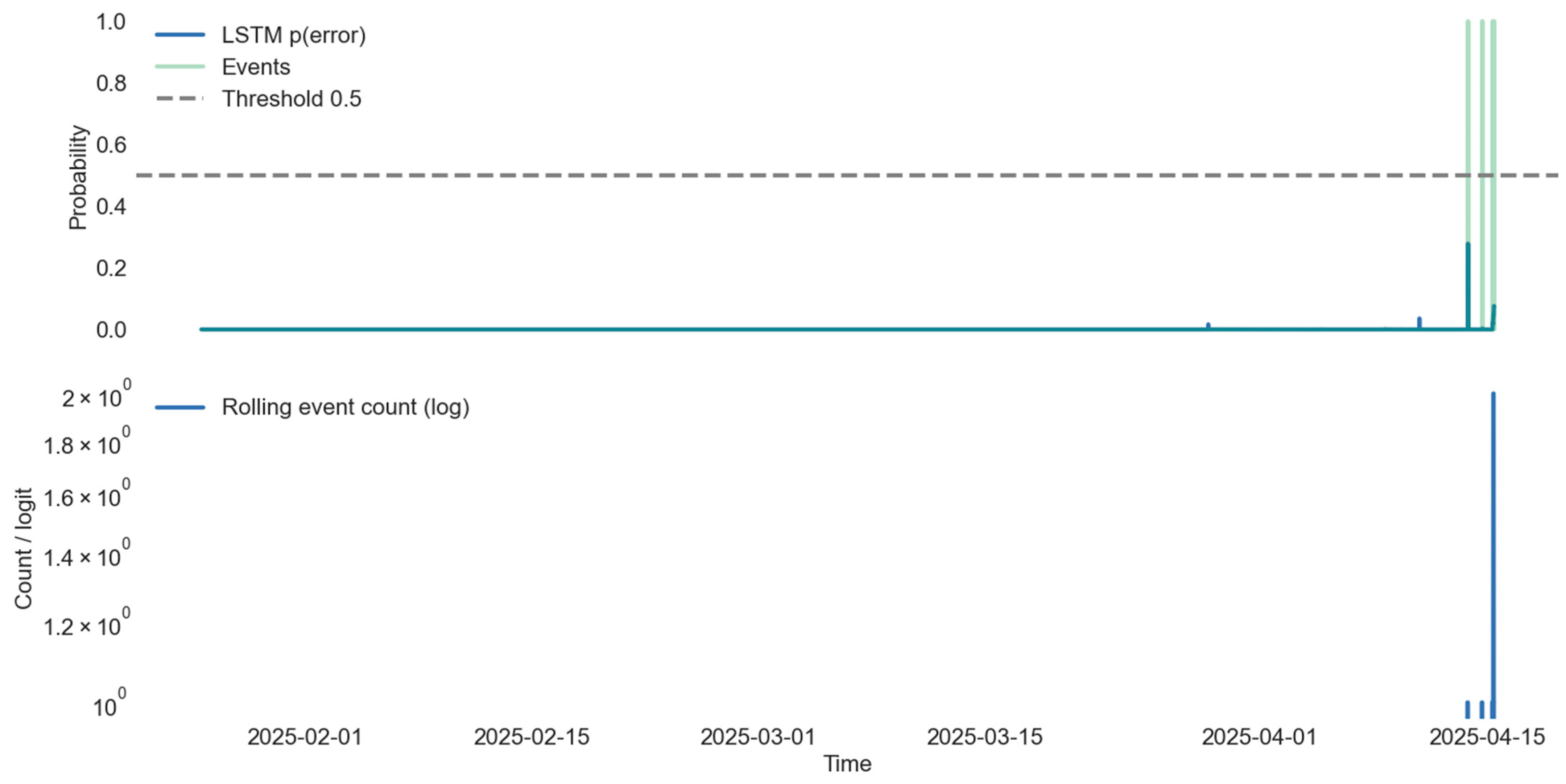
Figure 1 presents the result of training an LSTM model for predicting the probability of error occurrence. The time axis corresponds to the SCADA timestamps and is shown in calendar time, with a fixed sampling interval of five minutes.

Real errors are reported as rare and short-lived events, concentrated at the beginning of the observed period. This is a typical problem in reliability analysis, as failure/incident type events are significantly less common compared to normal operation [33]. The LSTM prediction shows high probabilities at the moments coinciding with real errors, while outside them, the values remain close to zero. This suggests that the model can distinguish normal from abnormal states despite class imbalance.

It is observed that for longer error-free periods, the model predicts with zero probability, which can be interpreted as a conservative strategy to avoid false alarms. This effect is useful in predictive maintenance systems, but at the same time emphasizes the need for class balance techniques (oversampling such as SMOTE, cost-sensitive learning, class-balanced loss) [34,35] and for adequate imbalance metrics (PR-AUC, instead of just ROC-AUC; MCC) [36,37].

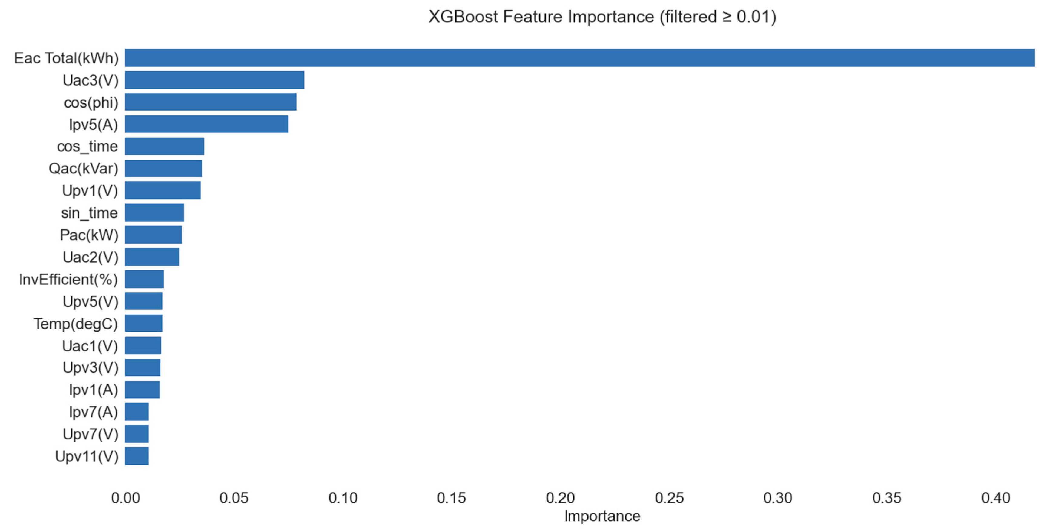
Figure 2 presents an analysis of the significance of the features calculated using an XGBoost model trained for binary classification of inverter states (normal operation vs. error/anomaly). The results show that the greatest influence on the model is exerted by the following:

• Inverter efficiency (InvEfficient (%)) with a share of over 28%;
• Total AC energy produced (Eac Total) is around 30%;
• DC and voltage measurements (especially from individual PV strings—Ipv3, Ipv8, Upv9);
• Inverter temperature (Temp (degC)) and output active power (Pac (kW)).

Of lower, but not negligible, importance are the time characteristics (sin_time, cos_time) which help capture the cyclic behavior of the PV system.

This analysis highlights variables that are most influential for the classifier in the analyzed dataset. In particular, efficiency/energy yield and string-level currents/voltages appear informative for distinguishing normal from incident-related behavior.

The resulting weights serve as the basis for building an HI, and they can be further validated by interpretability, e.g., SHAP [38], in addition to feature importance of XGBoost [18] and RF [39].

The correlation analysis is included as a supporting exploratory step to characterize relationships among key SCADA variables and to motivate the construction of the correlation-based drift indicator. The observed correlation patterns largely reflect expected physical and operational couplings between electrical, thermal, and performance-related quantities.

Rather than interpreting individual correlation coefficients as standalone findings, the analysis is used to establish a baseline structure against which temporal deviations can be assessed. In this context, the emphasis is placed on the evolution of correlation patterns over time, summarized through the drift indicator, which is subsequently evaluated as part of the hypothesis-driven analysis.

The correlation results are therefore interpreted as contextual information that supports feature selection and drift detection, and not as independent evidence of reliability or degradation mechanisms.

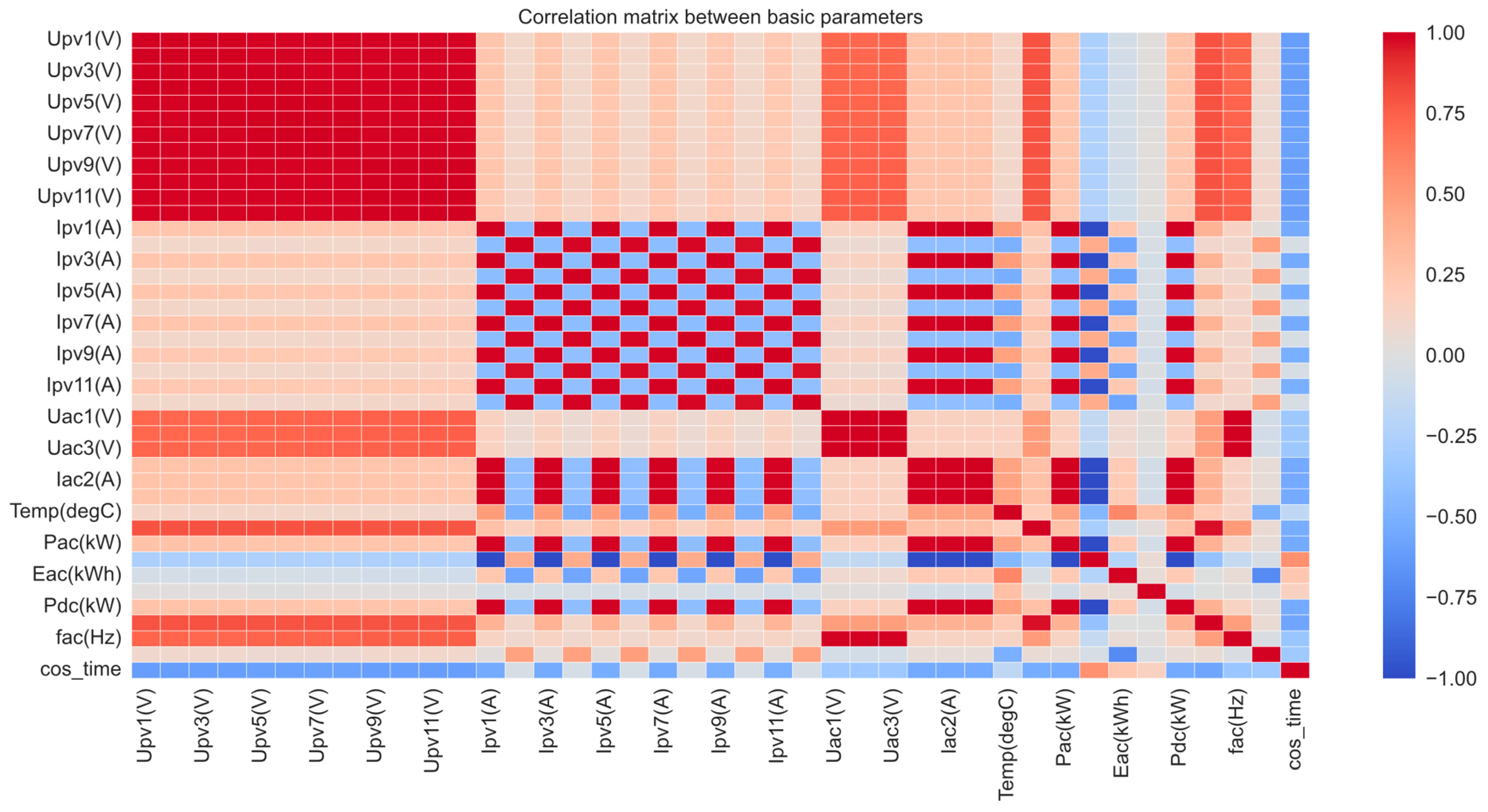
Figure 3 presents a matrix of correlations between the key measured quantities: voltages (Upv), currents (Ipv), active and reactive power (Pac, Pdc), efficiency (InvEff), frequency (fac), and temperature. We observe the following:

• Strong positive correlation (>0.9) between the voltages of the different PV strings (Upv1, Upv3, Upv5…), which is expected due to the general lighting conditions;
• Strong positive correlation between the currents of the individual strings (Ipv3, Ipv7, Ipv9), which indicates their synchronous behavior;
• High correlation between Pac and Pdc, which suggests that the output AC power follows the input DC power;
• Negative correlation between efficiency (InvEff) and temperature (Temp (degC)), which illustrates the typical reduction in efficiency at higher temperatures [39,40];
• Weak-to-moderate correlation between frequency and the other parameters, which is logical since the frequency is regulated by the grid.

The analysis of this matrix allows us to define correlation indicators for reliability. Changes in these relationships over time motivate the use of a correlation-drift indicator as a screening signal for potential deviations that may warrant further inspection.

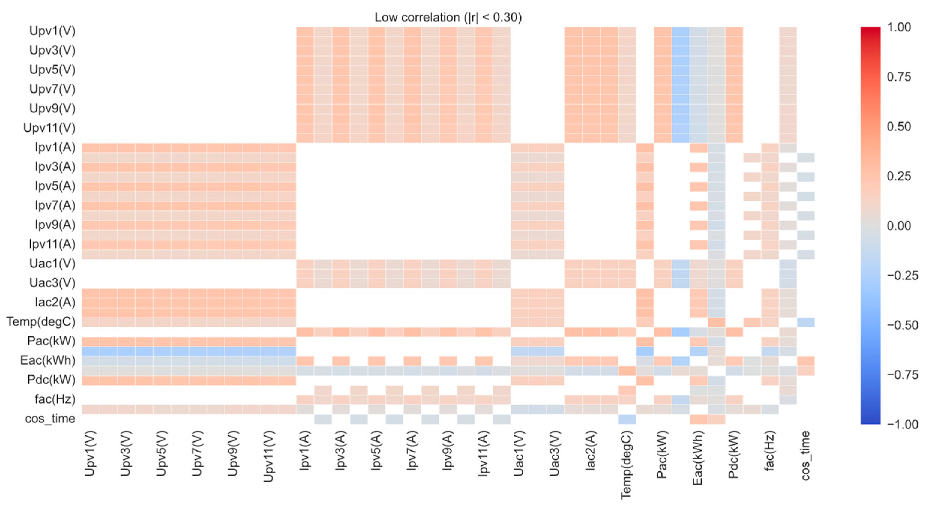
The heat map in Figure 4 shows only pairs of variables with weak correlation (absolute correlation below 0.30), with the main diagonal excluded. Most combinations between PV string voltages/currents (Upv*, Ipv*), grid quantities (Uac*, Iac*), frequency fac (Hz), active power Pac (kW), DC power Pdc (kW), stored energy Eac (kWh), temperature Temp (degC), and time codes (sin_time, cos_time) remain in the range 0.00–0.28. Weak positive relationships are mainly observed around r ≈ 0.20–0.28. Weak negative relationships are most noticeable between Temp (degC) and some of the energy/time quantities (e.g., r ≈ −0.17–−0.28).

This view supports feature selection by highlighting weakly coupled variables that may provide complementary information and reduce redundancy.

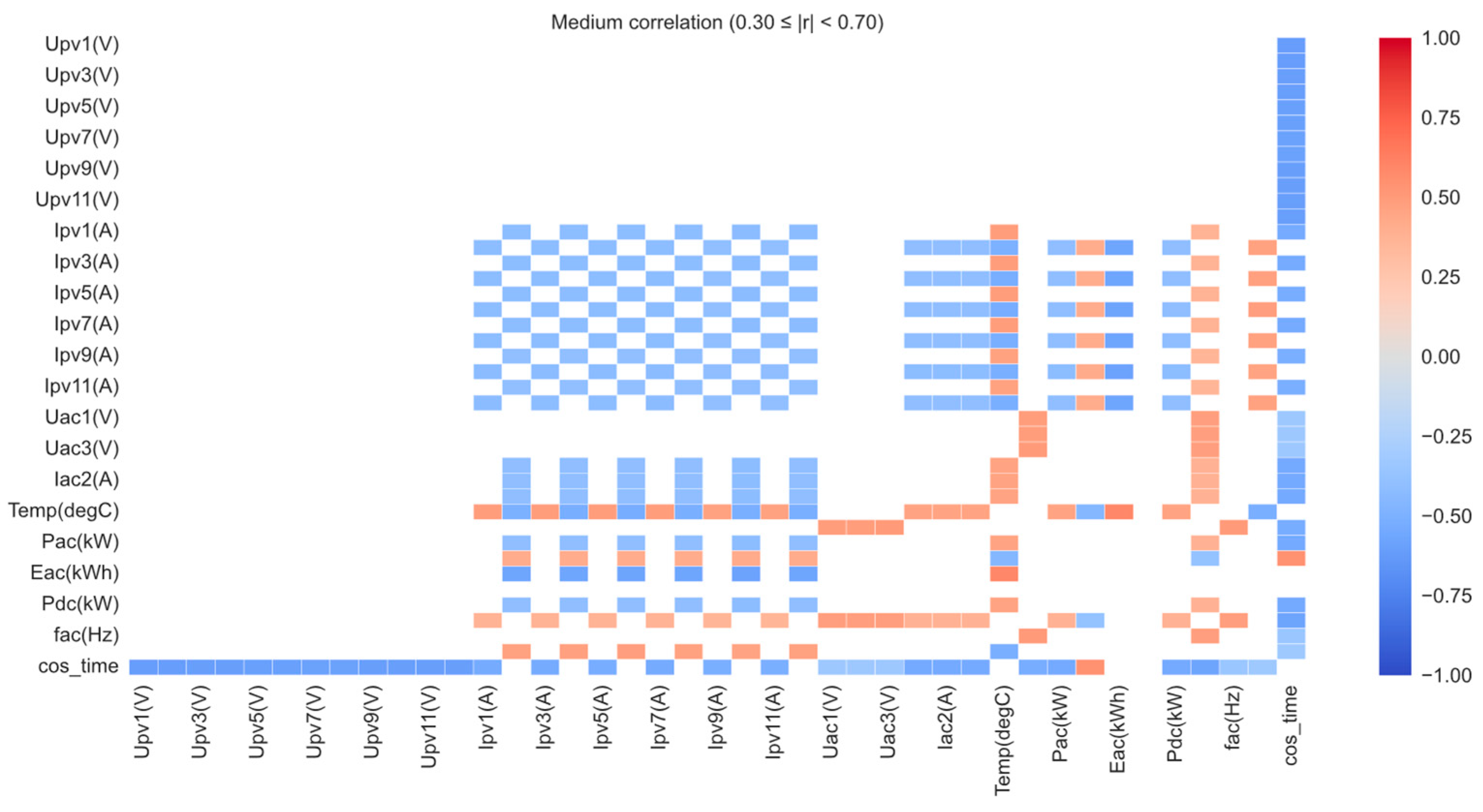
Figure 5 shows pairs of quantities with moderate absolute correlation. The main observations are that the temperature Temp (degC) has a positive average relationship with the energy/power parameters Pac (kW), Pdc (kW), Eac (kWh) (≈0.46–0.50). This reflects an increased thermal load at higher production. Positive correlations are seen between Pac–Pdc–Eac in the range 0.38–0.51, which is expected for the AC/DC power chain, but still under “high” power (i.e., the relationship is not perfect and remains sensitive to efficiency and network effects). A part of the PV currents Ipv* shows a negative average correlation (≈−0.40–−0.43) with individual voltages/parameters, which indicates the typical current–voltage trade-off at different operating points and loads. Fac (Hz) has a weak-to-moderate positive correlation with some features (up to ≈0.51), without a systematic strong dependence, logical for grid-controlled frequency. The time code cos_time correlates positively with parts of the PV voltages (≈0.55–0.61), capturing the diurnal cycle of illumination.

The figure with average correlations highlights that thermal influence on production, with incomplete interchangeability between AC/DC indicators useful for feature selection, as well as diurnal regularities that should be modeled by sin/cos time codes. Tracking these relationships over time is suitable for detecting correlation drift and early signs of operational deviation from baseline behavior.

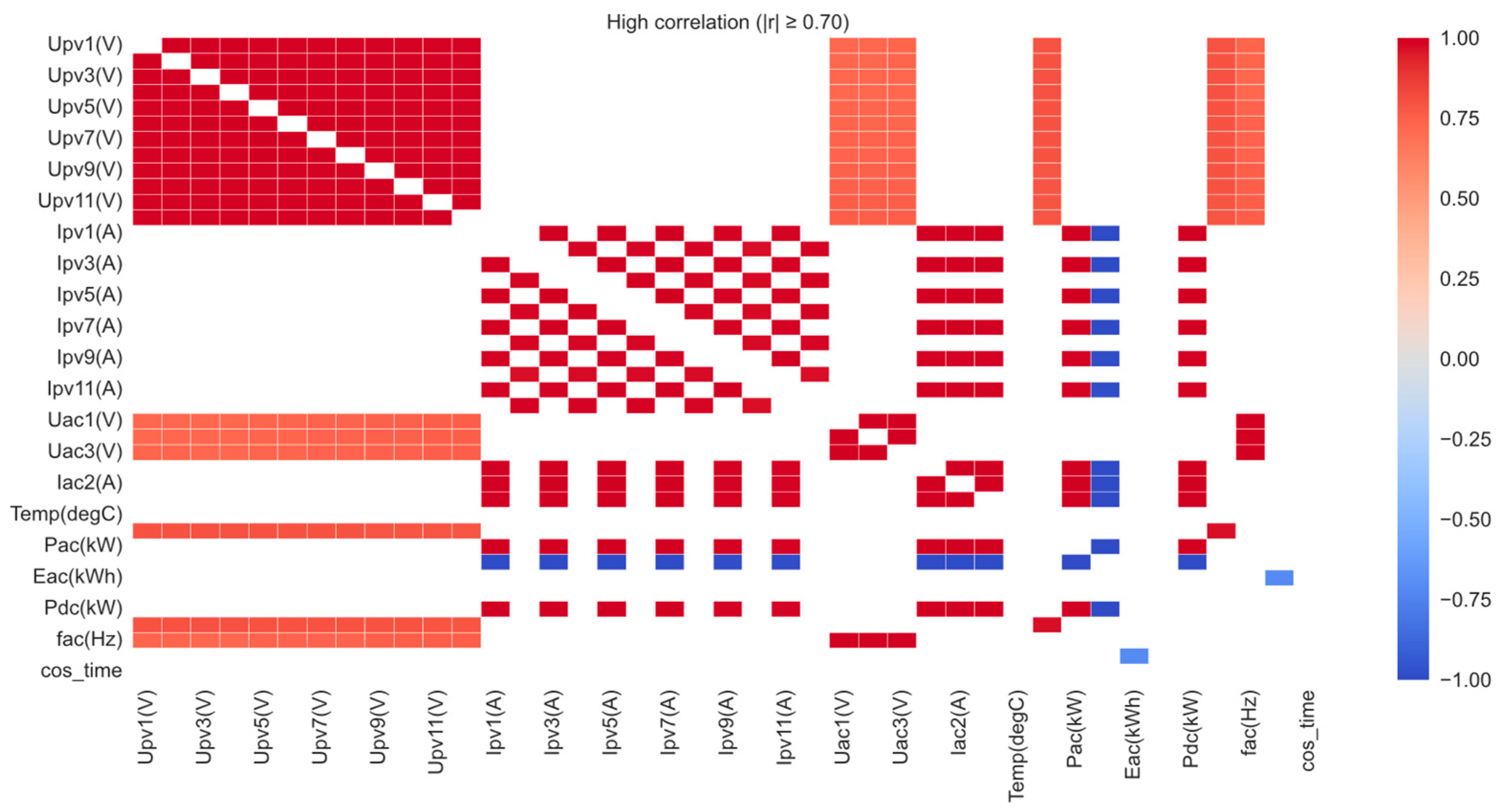
Figure 6 shows a heat map showing the most strongly correlated pairs of quantities. Three “clusters” are clearly visible. PV voltage block (Upv*): The voltages of the individual strings are very strongly positively correlated (typically r ≳ 0.90). This is expected under general conditions of illumination/temperature and homogeneous strings. PV current block (Ipv*): The currents of the strings are strongly positively correlated (r ≳ 0.85–0.95), reflecting their synchronous response to radiation and partial shading. High collinearity suggests redundancy; for modeling, a representative subset is often sufficient. Power block (Pdc, Pac, Eac): Pdc Pac is extremely positively correlated (often r ≳ 0.95), and Eac is also strongly correlated with them (especially with a longer aggregation window). This reflects the DC/AC sequential connection and the consistent operation of the conversion.

In some periods, a strong negative correlation is observed between the efficiency of InvEff and the temperature Temp (degC) (often |r| ≳ 0.70), which is physically justified (decrease in efficiency during heating). The frequency fac (Hz) does not participate in strongly correlated pairs; it is network-driven and almost independent of the other indicators in normal operation. The phase voltages Uac1/2/3 usually do not jump in the zone |r| ≥ 0.70 with each other (except in highly symmetrical sections); this is an indicator of real network variations and phase imbalance when there is no strong connection.

There is high multicollinearity in the PV subspaces (Upv, Ipv, Pac/Pdc/Eac), which allows for a reduction in the measurement set (e.g., through PCA/feature selection) without loss of information. Transitions from high to medium/low in key pairs (e.g., Pdc–Pac or within-string voltage/current couplings) can be used as screening cues for deviations from baseline behavior. Attributing these changes to specific physical causes requires additional context (e.g., maintenance logs or dedicated diagnostics).

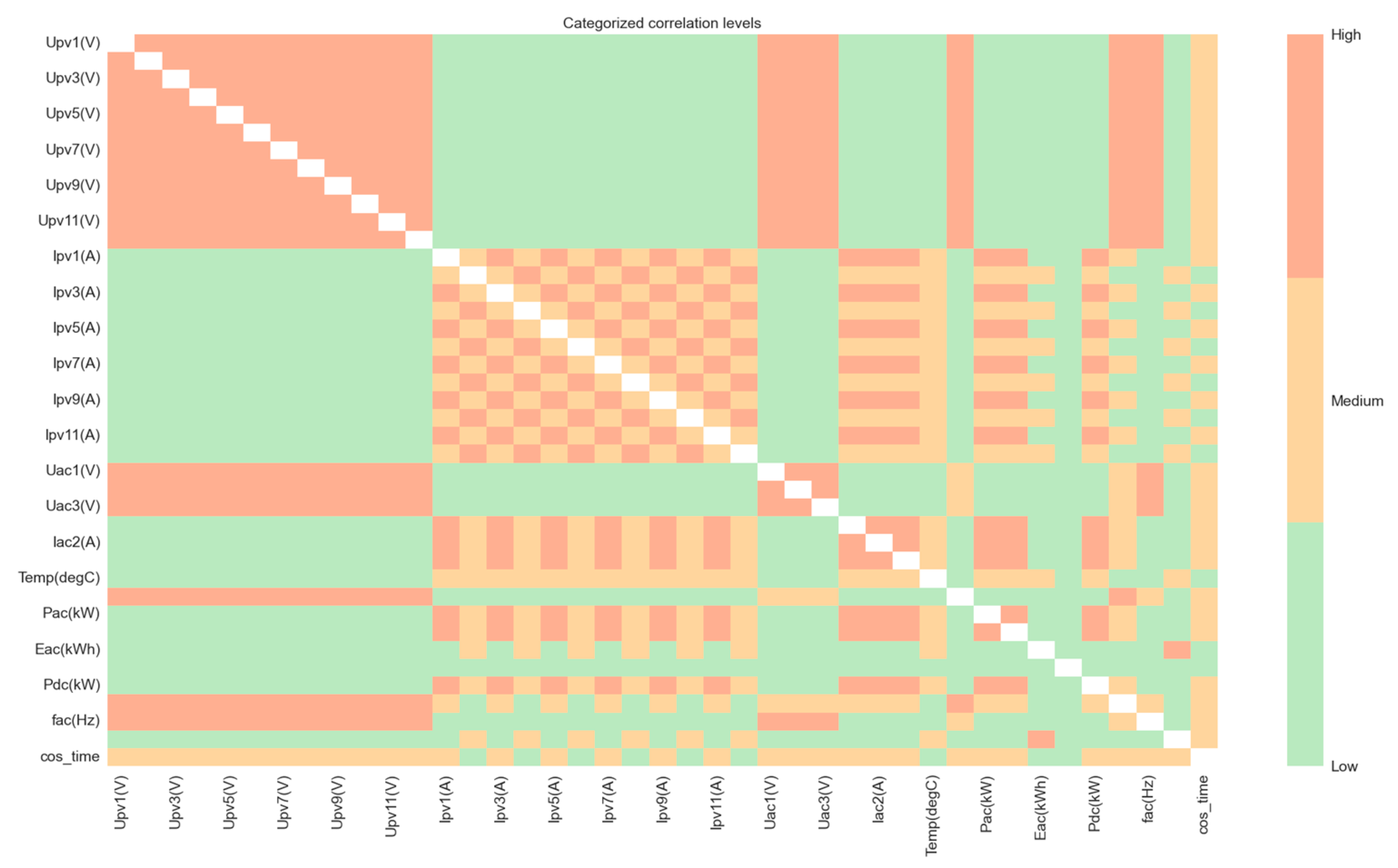
Figure 7 shows the same correlation matrix, but discretized by three thresholds: low (|r| < 0.30, green), medium (0.30 ≤ |r| < 0.70, orange), and high (|r| ≥ 0.70, red). This shows the “blocks” of interdependence without being distracted by the exact numerical values. PV voltages (Upv*) form a dense high block among themselves and a strong covariance is expected due to the general illumination/temperature. PV currents (Ipv*) form a mosaic of high and medium blocks, indicating a strong but slightly more unstable correlation (due to the influence of partial shading and uneven losses). The energy–power triplet (Pdc, Pac, Eac) is mostly high, which suggests the sequential dependence of DC/AC and the accumulation in energy. Temperature (Temp (degC)) against the energy–power indicators is most often seen as medium (often negative when viewed in detail), which is in line with decreasing efficiency during heating. Phase voltages Uac1/Uac2/Uac3 are mainly medium/low among themselves, which is an indicator of real network variations and possible phase asymmetries. Frequency (fac (Hz)) remains low to almost all values, with some being network-driven and others being weakly dependent. The time characteristic cos_time falls mainly into low/medium, i.e., carries cyclical, but not dominant information.

The dense high blocks (Upv, Ipv, Pdc–Pac–Eac) allow compression (e.g., PCA/selection of representative channels), without loss of informativeness. Transitions from high to medium/low in key pairs can be used as screening cues for deviations from baseline behavior and should be interpreted jointly with model-based indicators and event labels. Temperature interactions (nedium) justify a higher weighting of Temp and InvEff in the HI, while fac (Hz) can be treated as a separate control indicator.

The following sections build on this exploratory analysis by focusing on model-based indicators and their evaluation under a structured, hypothesis-driven framework.

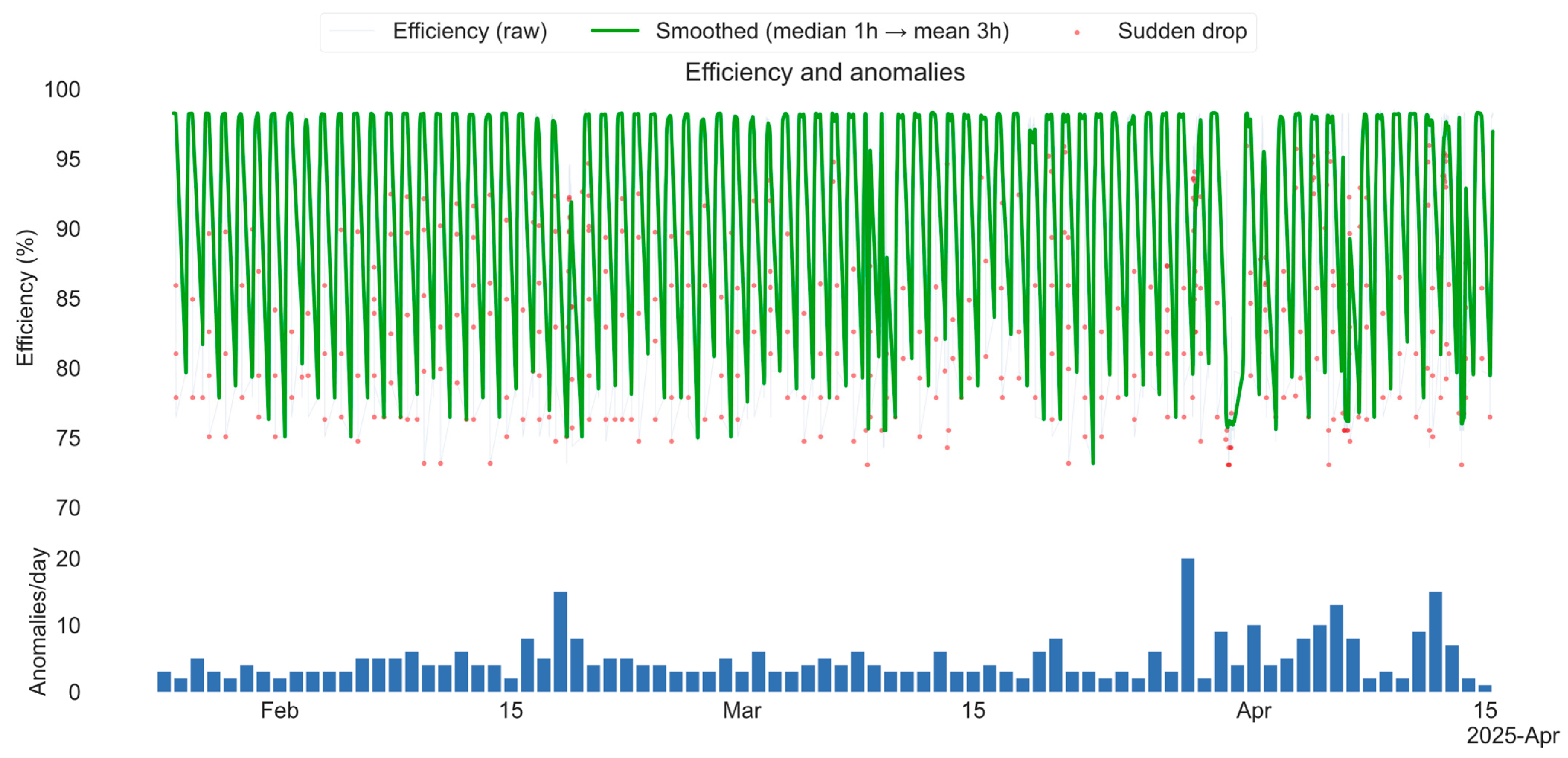
Figure 8 shows the time evolution of the inverter efficiency for the period February–April 2025. It is observed that despite maintaining high average efficiency values (~85–95%), multiple short-term deviations appear. These “dips” can be associated with temperature peaks and overheating of the power elements, which is transient in the network, such as problems in individual PV strings, leading to temporary loss of power.

The lower panel (blue bars) shows the daily count of detected efficiency-drop anomalies, aggregated from the high-resolution time series. Regular detection of such anomalies is of particular importance, as they signal potential operational deviations that may warrant closer inspection, even when the overall efficiency remains within acceptable limits.

This visualization motivates the benefit of combining instantaneous values and smoothed trends, as it allows for simultaneous capture of short-term deviations, while tracking the overall trend [40,41]. Including these indicators in the HI improves the sensitivity of the reliability assessment system [42,43].

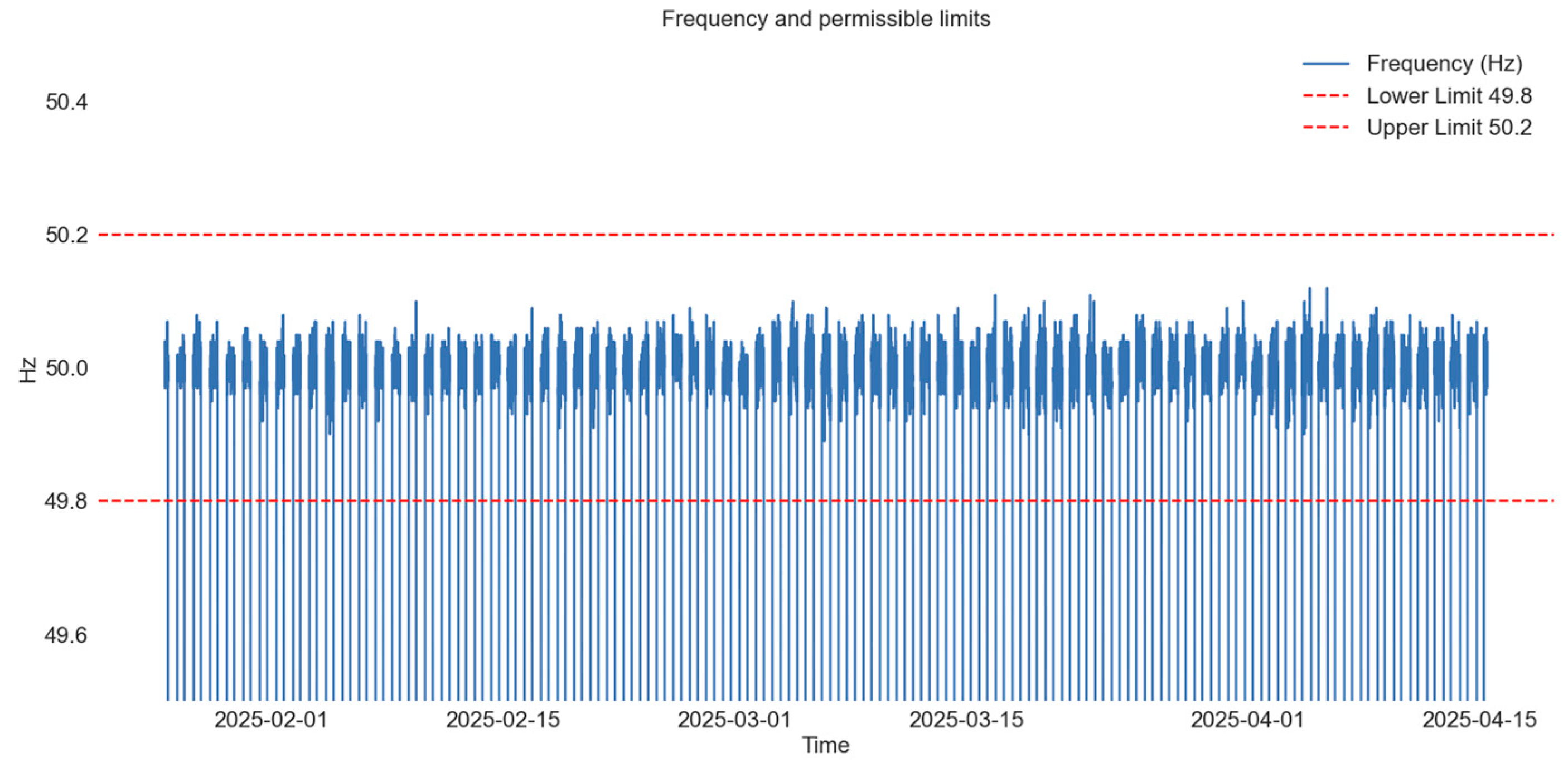
Figure 9 shows the dynamics of the inverter output frequency (fac (Hz)) during February–April 2025. Over the analyzed period, the frequency remains within the regulatory limits, without prolonged deviations. This behavior is consistent with stable grid synchronization under the observed operating conditions. Short-term variations around the nominal value (50 Hz) are expected and reflect normal power–system dynamics. Overall, the frequency profile does not suggest persistent power-quality disturbances in this dataset.

Frequency deviation is included among the HI risk indicators to capture potential grid-side disturbances when they occur; in this case, study periods with such deviations appear limited.

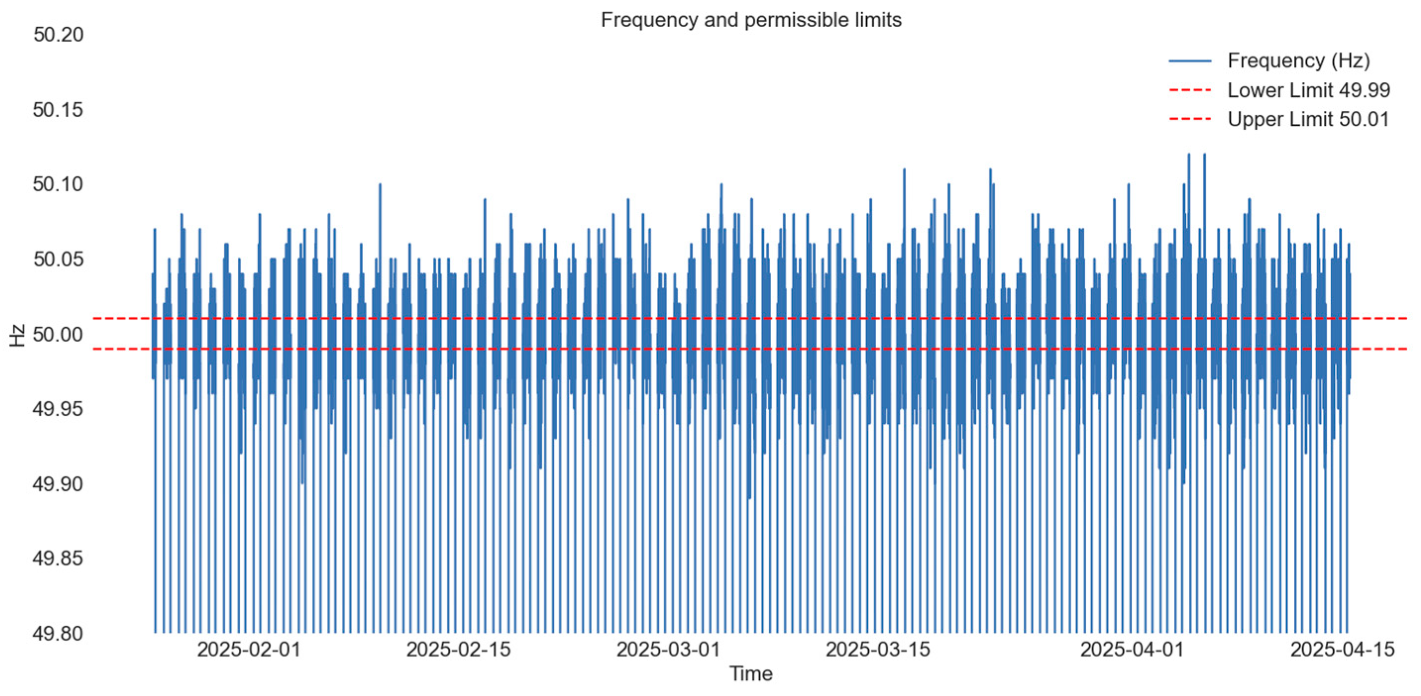
Figure 10 presents the same frequency signal with narrower tolerance limits (49.99–50.01 Hz). Most samples remain within this band, with occasional short excursions of low amplitude and short duration. Such excursions are typically not critical on their own, but if they persist, they may indicate changes in grid conditions or control behavior. In the analyzed dataset, the tightened-band view provides a more sensitive check for short-lived deviations and supports the interpretation of frequency as a secondary monitoring variable.

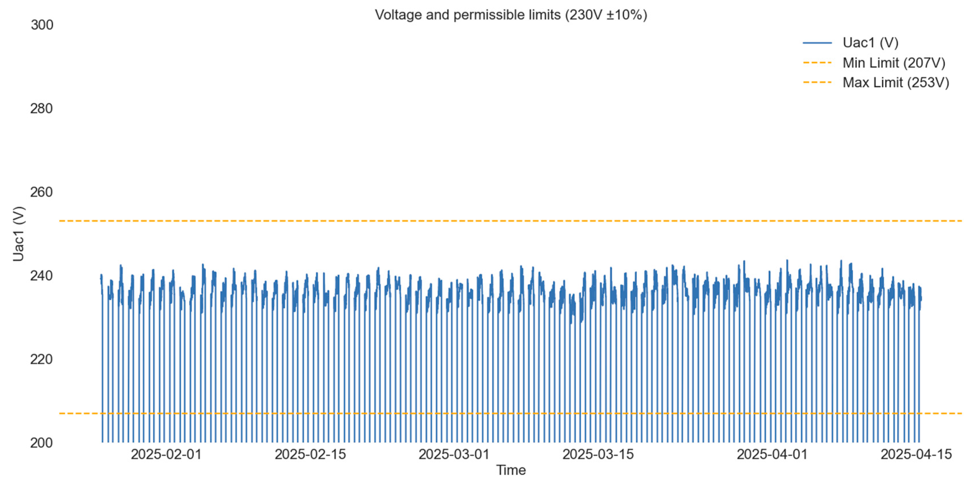
Figure 11 shows the first-phase voltage (Uac1) over February–April 2025. The voltage remains within the regulatory limits, with short-term variations that are typical for normal grid operation. While prolonged deviations outside the permissible range can increase thermal stress and affect conversion efficiency, such sustained excursions are not observed in this case study period. Uac1 is therefore treated as a contextual electrical indicator included in the HI feature set.

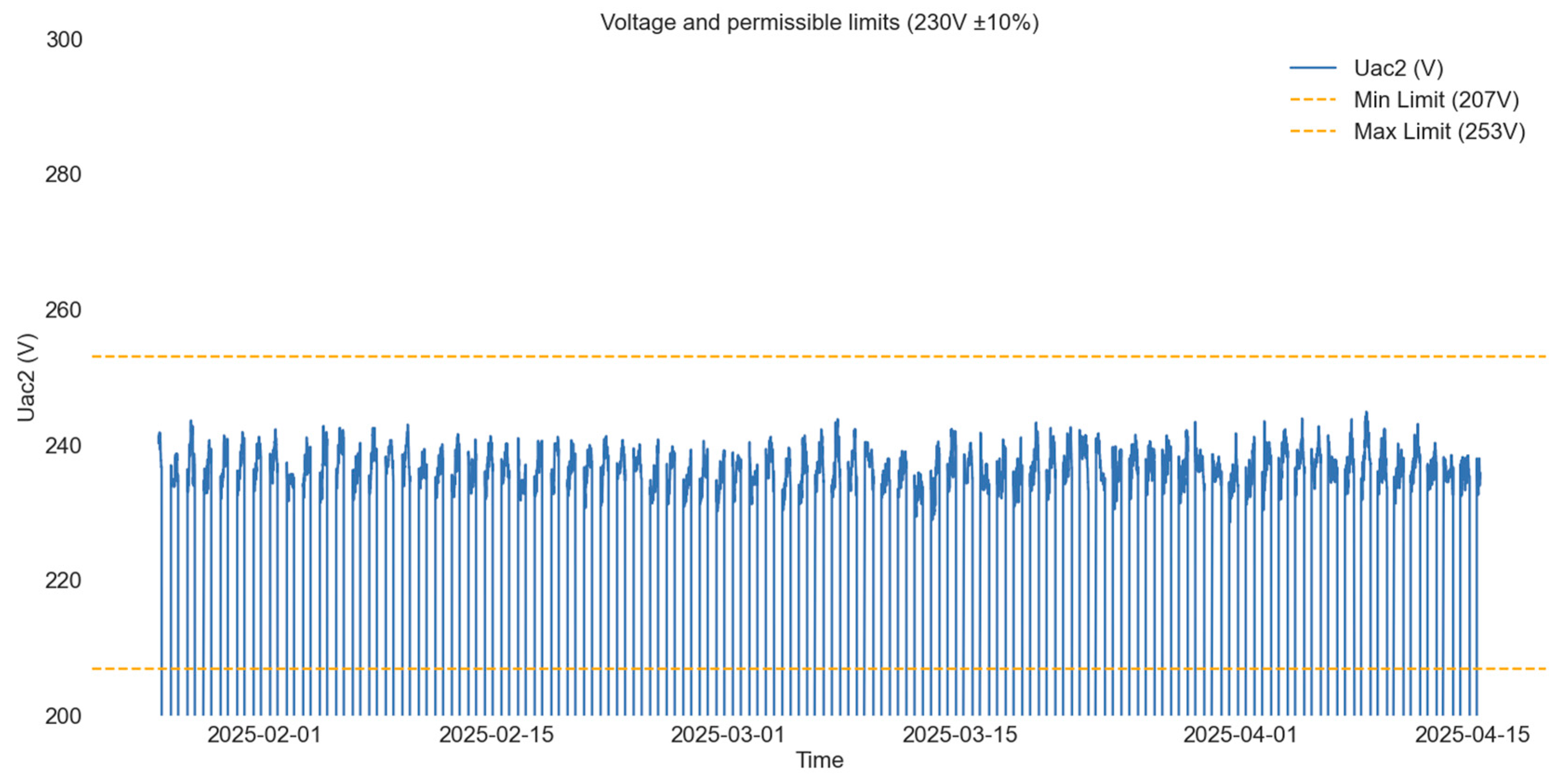
Figure 12 shows the second-phase voltage (Uac2) for the same period. The signal remains within limits with fluctuations comparable to Uac1, which is consistent with typical phase–voltage behavior under the observed conditions. In this dataset, no sustained out-of-band intervals were observed. Monitoring all phases remains important, as persistent phase imbalance or asymmetric loading can increase stress on power electronics.

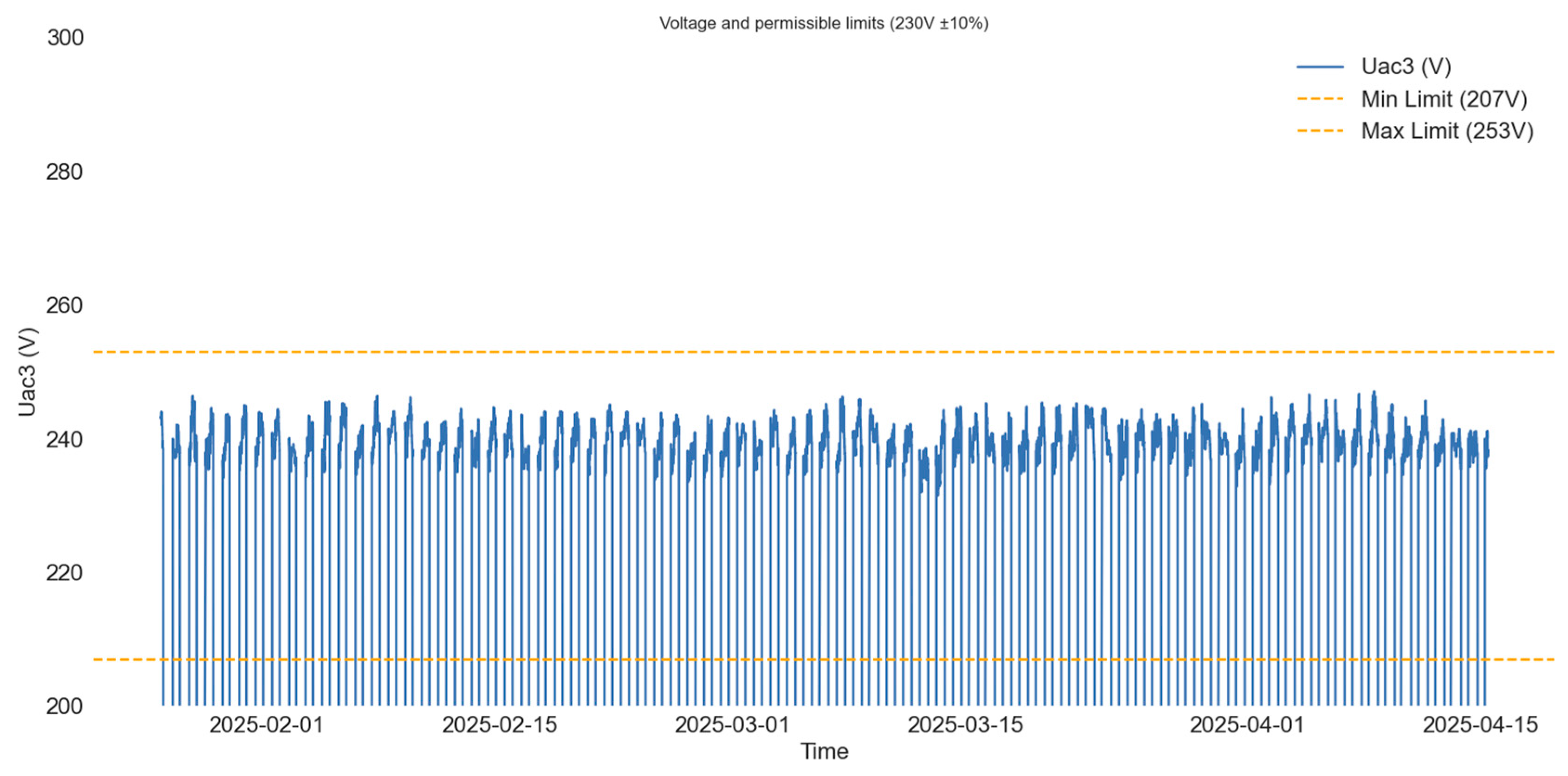
Figure 13 presents the third-phase voltage (Uac3). Similarly to Uac1 and Uac2, the voltage remains within the permissible range without long-term deviations in the analyzed period. The three-phase view provides a practical check for potential asymmetries; although significant phase imbalance can increase thermal stress, such patterns are not prominent in this case study dataset. Including phase voltages that in HI help reflect electrical operating conditions alongside temperature, efficiency, and frequency indicators.

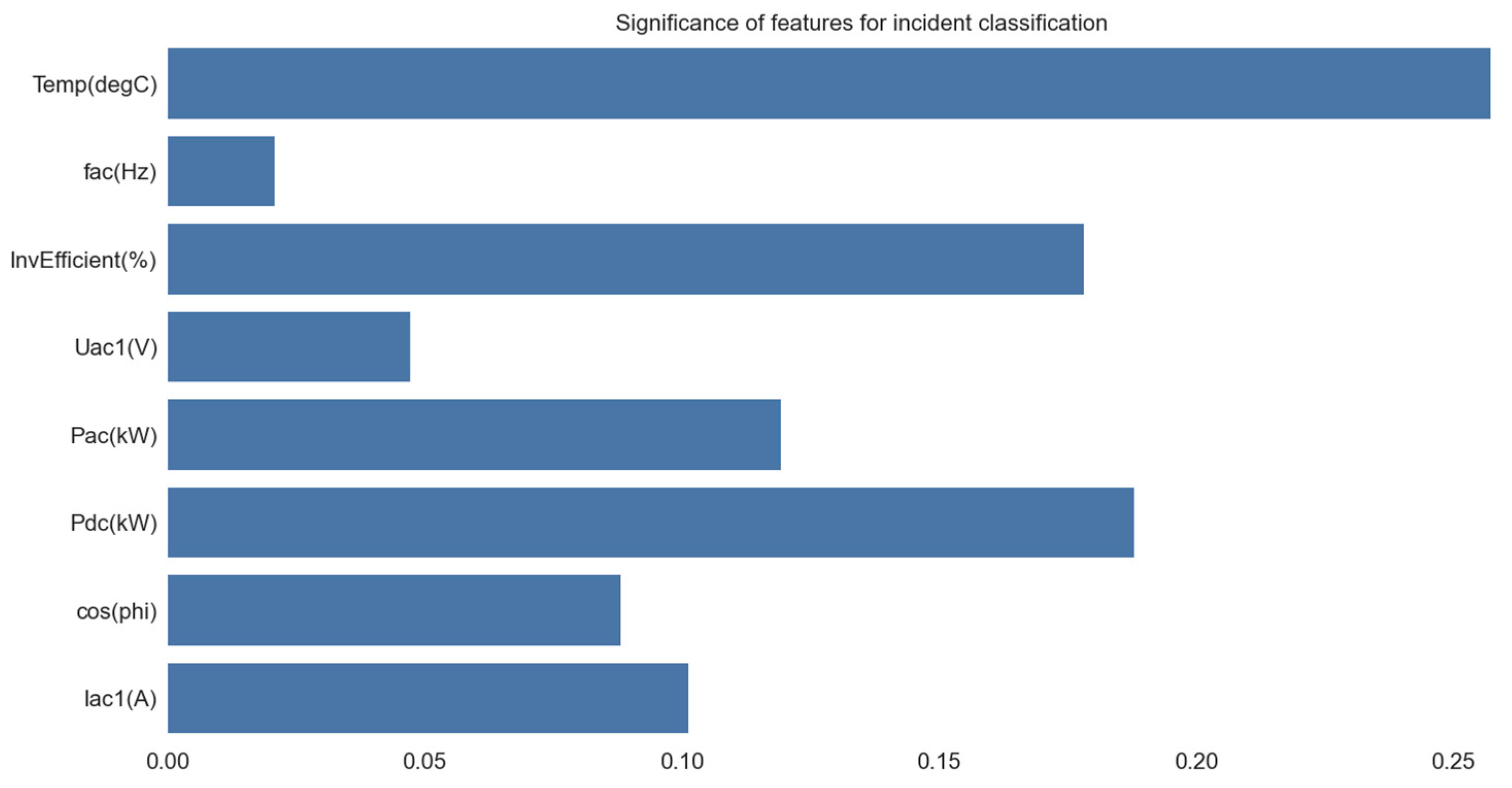
Figure 14 presents the results of training an RF model for incident-type classification based on SCADA data. The following parameters have the highest importance: Inverter temperature (Temp (degC)), with the largest contribution (~25%), which highlights its critical impact on reliability and failure risk. DC power (Pdc (kW)) and efficiency (InvEfficient (%)), which also occupy leading positions, as they reflect the energy behavior and conversion losses. Output active power (Pac (kW)) and first-phase current (Iac1 (A)), which provide information about the load and state of the AC side. Power factor (cos (phi)) and first-phase voltage (Uac1 (V)), which play a supporting but significant role in the identification of deviations.

A lower, but still significant, weight has the frequency of (fac (Hz)), which under normal conditions remains consistent and is therefore less often used as a primary indicator of incidents.

The results show that temperature and efficiency are dominant factors, while the combination of power and electrical parameters helps in more accurate classification of incidents. This information was used in the construction of the HI, by assigning appropriate weights to the indicators. The RF outputs that match XGBoost, Temp, InvEff, Pdc are leading.

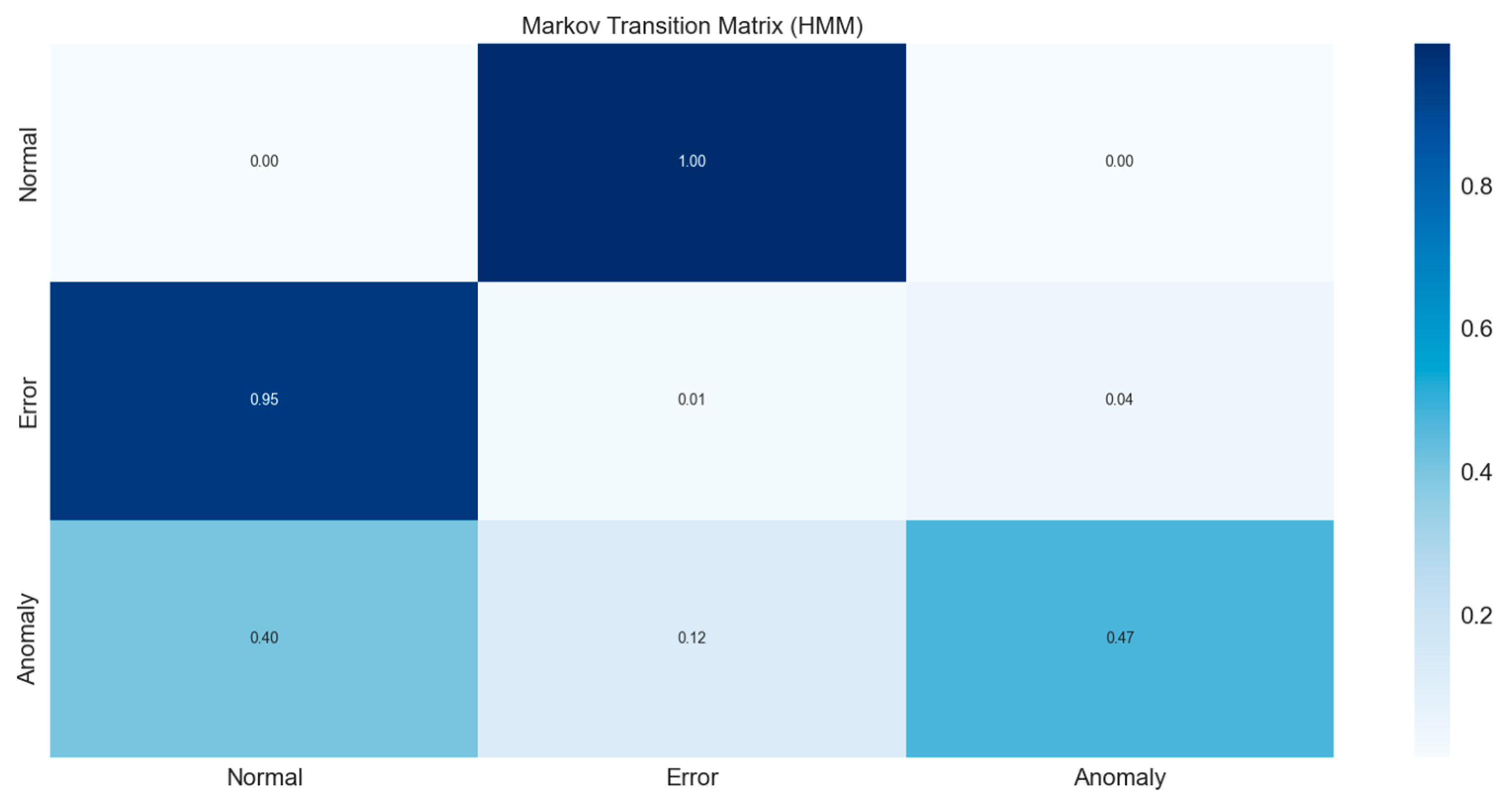
Figure 15 presents the transition probabilities between the three defined inverter states, namely Normal, Error, and Anomaly, estimated using a hidden Markov model. The main observations are that the Normal state transitions to Error with 100% probability, indicating that in the presence of an error, the transition is direct and abrupt. The error state has a high probability (95%) of returning to normal, meaning that errors are usually short-lived and recoverable. Transitions to anomaly are rare (4%). The anomaly state has a relatively high probability of remaining in itself (47%) or transitioning to normal (40%). This indicates that anomalies are often self-dissipating, but in some cases (12%), they can escalate to an error (Error).

The interpretation of HMM-based results depends on modeling choices, such as the initialization of state probabilities and the number of hidden states chosen. To reduce over-interpretation and assess robustness under the case study setting, sensitivity analysis was considered for key HMM settings.

Given that the “Error” events in the analyzed dataset are concentrated towards the beginning of the observation period, the empirical initialization of π may reflect a bias from the beginning of the record. To address this, alternative initializations, including weakly informative or stationary priors, were considered to assess whether the observed state transition patterns remain qualitatively consistent.

The primary analysis uses a three-state configuration (Normal/Anomaly/Error) for interpretability and operational relevance. To assess sensitivity, alternative configurations with fewer or more states are conceptually considered and remain qualitatively stable within a reasonable parameter range. This analysis aims to verify that qualitative conclusions are not driven by a single arbitrary choice of state cardinality. In this study, the “Error” state is treated as an indicator of operational failure, rather than as a permanent failure state. The frequent transitions from “Error” back to “Normal” suggest that most events are transient. Accordingly, the HMM is not interpreted as a degradation mechanism or absorbing failure model, but as a probabilistic description of short-term operational states.

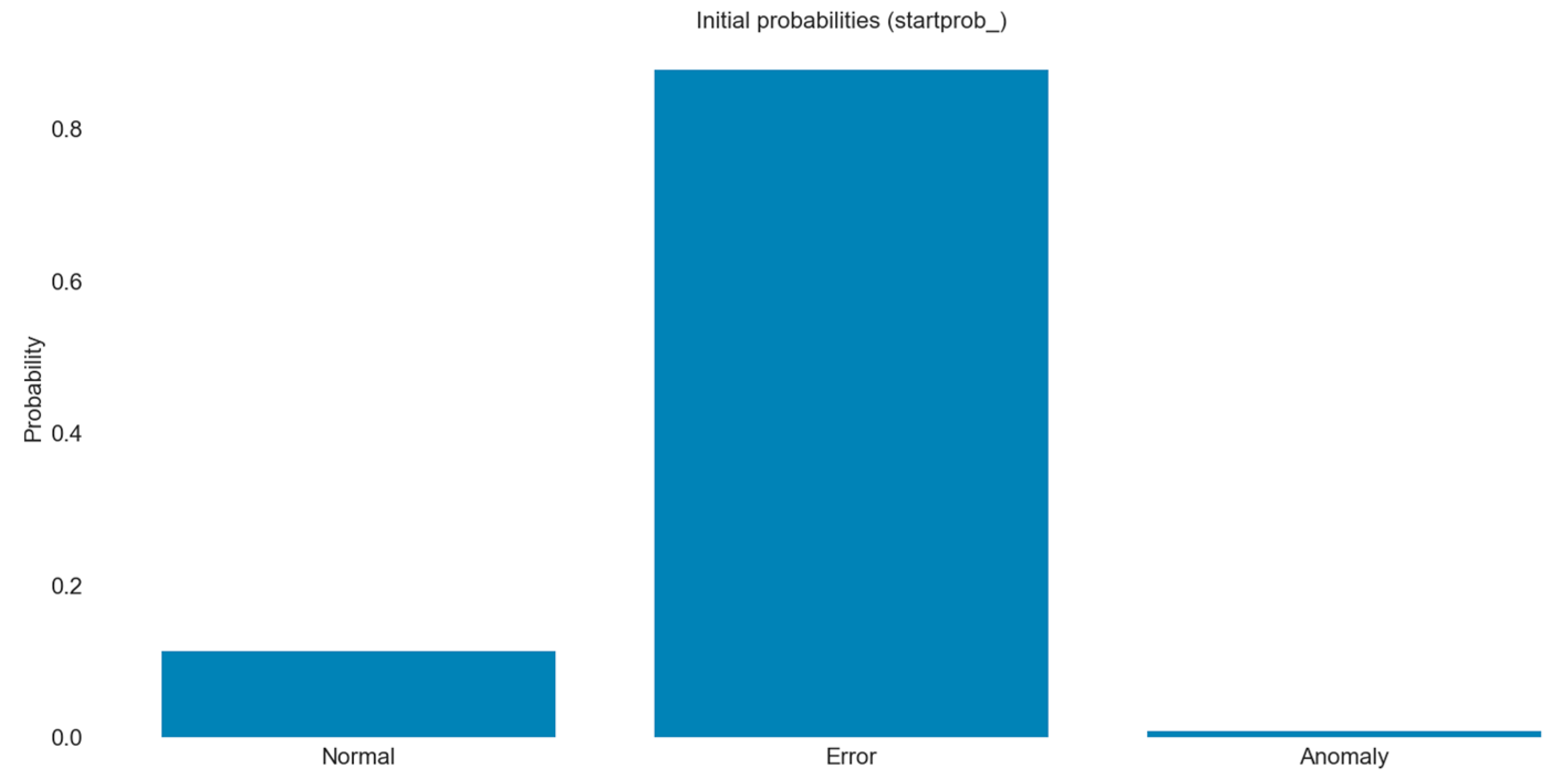
Figure 16 presents the initial probabilities for the three defined states, namely Normal, Error, and Anomaly, estimated by the HMM. The results show that the highest probability of the initial state is Error (about 85%), while the Normal state has a significantly lower initial probability (~12%); the Anomaly state practically does not occur as an initial state (<1%).

This behavior can be explained by the characteristics of the training dataset used, where the “Error” events are strongly marked at the beginning of the record. In practical application, the model can be calibrated by retraining with more balanced data, so that the initial probabilities reflect the real expected state of the system (normal operation as the dominant state).

This step is important for the correct construction of a predictive reliability model, as it affects the initial behavior of the simulations and the predictions of future transitions between states.

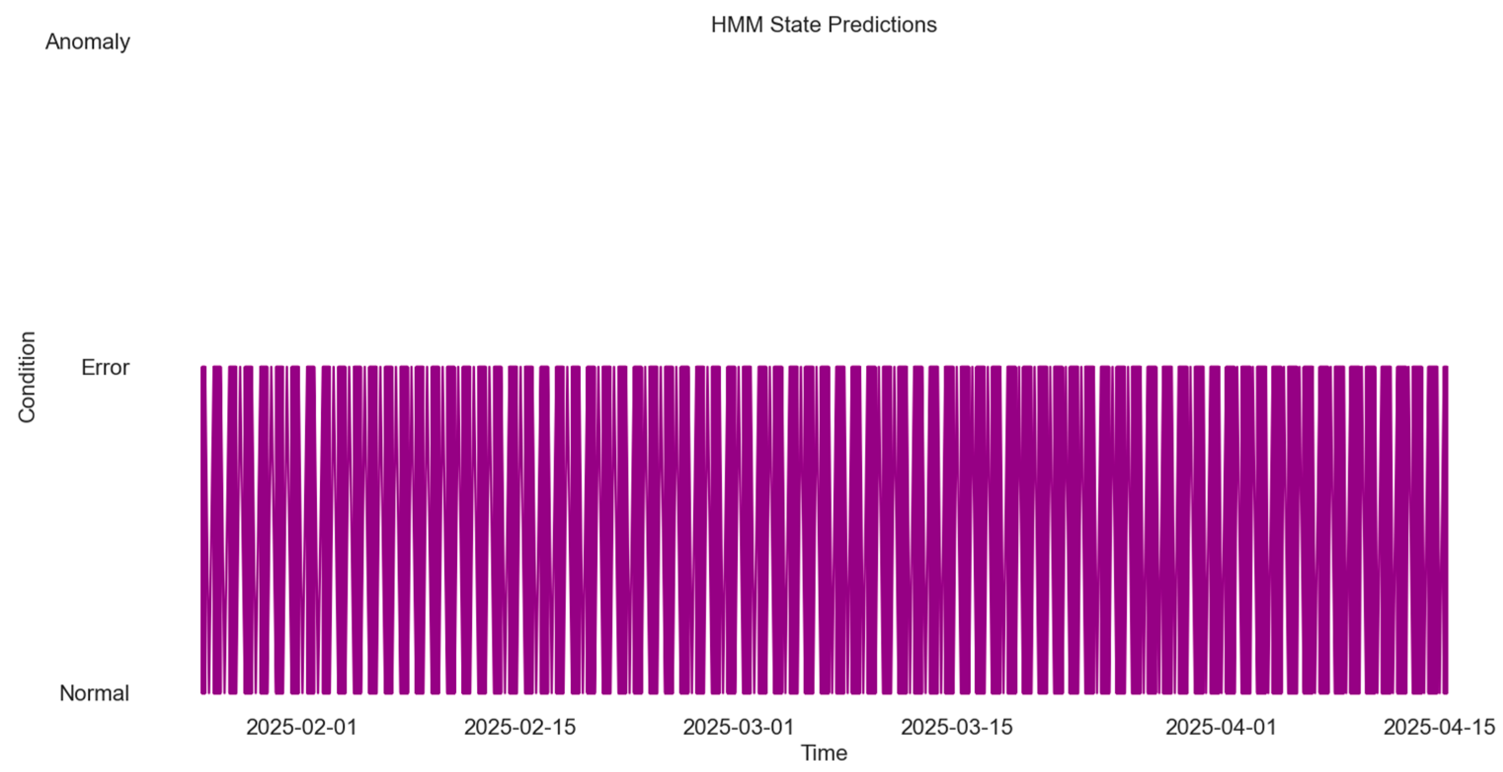
Figure 17 shows the predicted states of the inverter (Normal, Error, Anomaly) obtained from the HMM for the period February–April 2025. The results show dominance of the transitions between Normal and Error, which is consistent with the observations from the transition matrix. This is consistent with the observation that a large part of the errors is transient, and the system quickly restores its normal operation. Regarding long-term anomalies, the Anomaly state does not persist over long intervals, which is consistent with its limited presence in the analyzed period. This time dependence is useful for summarizing temporal behavior and for supporting the interpretation of changes in the inferred risk level when combined with the model-based indicators.

Table 2. Sensitivity considerations for the HMM configuration.

Aspect	Configuration Considered	Purpose
Initial probabilities (π)	Empirical vs. weakly informative	Reduce start-of-record bias
Number of states	K = 2, 3, 4	Assess the robustness of state interpretation
Error state modeling	Transient (non-absorbing)	Avoid over-interpretation as failure

summarizes the key HMM configuration aspects considered in the sensitivity analysis, including initial state probabilities, the number of hidden states, and the interpretation of the Error state.

Table 2 outlines sensitivity considerations to bound interpretation of HMM results under the case study setting, rather than providing an exhaustive robustness analysis.

The warning thresholds and critical values κ used to construct the HI and RS were initially motivated by expert knowledge and operational practice. To reduce subjectivity and improve reproducibility, a sensitivity analysis framework is considered to assess how variations in κ affect the behavior of the indicator and the alarm characteristics.

The analysis examines a limited range around the nominal values of κ and examines the resulting trade-offs between detection sensitivity and false alarm rate. Rather than identifying a single optimal threshold, the goal is to verify that the qualitative behavior of the HI/RS and the relative interpretation of operational states remain qualitatively stable within a reasonable parameter range.

Given the scope of the case study and the limited observation horizon, the sensitivity analysis is interpreted as a robustness check rather than a final threshold optimization.

Table 3. κ-threshold sensitivity considerations.

Aspect	Description
Nominal κ values	Expert- and standard-based thresholds
Sensitivity range	Bounded variation around nominal values
Evaluation focus	Detection vs. false alarm trade-off
Interpretation	Robustness check within case study scope

frames κ-threshold sensitivity as a robustness check, not as an optimization or final threshold selection.

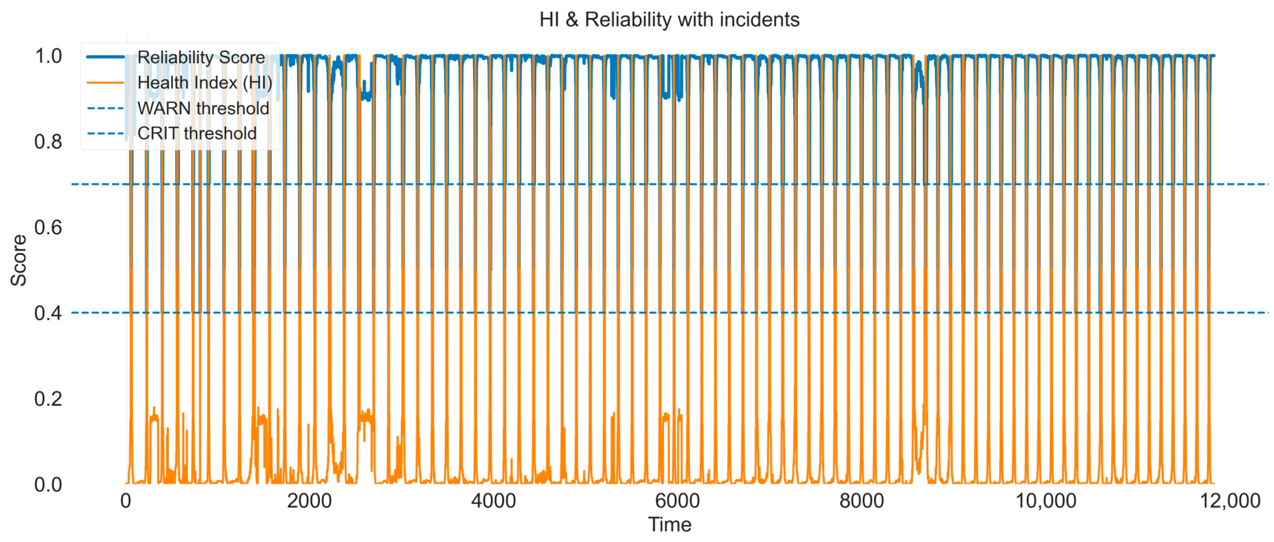
Figure 18 presents the dynamics of HI and RS over the observed period with WARN (0.7) and CRIT (0.4) thresholds and annotated incidents. In this dataset, RS remains predominantly high, while HI exhibits larger short-term variability and occasionally crosses the warning threshold during brief deviations. The annotated incidents tend to coincide with local HI drops, which suggests that HI can help flag periods that warrant closer inspection. RS does not show prolonged drops below the critical threshold in the analyzed record, which is consistent with its role as a smoother summary indicator under these conditions. Overall, the combined view illustrates complementary use, with HI for short-term screening and RS for trend monitoring and prioritization, within the scope of this case study.

Throughout the paper, findings are reported as evidence within the dataset analyzed, and broader generalization is treated as future validation.

5. Discussion

The presented framework is a case study of SCADA-based reliability monitoring for a PV inverter from February to April 2025. The main goal is to integrate complementary evidence from correlation-based drift, supervised ML probabilities (XGBoost, LSTM), and temporal consistency via HMM, and to summarize them through two interpretable composite indicators, namely HI (short-term deviations) and RS (longer-term reliability proxy).

The results indicate that HI reacts to short-lived deviations, such as efficiency drops or voltage disturbances, while RS remains comparatively smoother and reflects longer-term operating stability. From an operational perspective, this separation can support two different actions: HI can trigger inspection or targeted checks, whereas RS can support higher-level prioritization and trend monitoring. Importantly, these indicators should be interpreted as data-driven risk summaries, not as direct physical measures of deviation patterns.

The HMM component adds a compact representation of state dynamics (Normal/Anomaly/Error) and enables discussion of temporal patterns through transition probabilities. In this dataset, the observed transitions suggest predominantly transient events, which is consistent with the frequent return from “Error” to “Normal” and the limited persistence of the “Anomaly” state. However, the interpretation of HMM results depends on modeling choices (e.g., initialization and the number of states), and therefore, the HMM output is best treated as supporting evidence rather than a standalone reliability claim.

Compared to classical reliability indicators derived from historical failure and repair logs (e.g., MTBF/MTTR), the proposed workflow focuses on near-real-time context from SCADA measurements and aims to capture short-term risk events and evolving conditions. This does not replace classical reliability analysis; rather, it provides a complementary, operational layer that can be used when detailed maintenance logs are limited or when short-term monitoring is required.

Several limitations should be emphasized. First, the study covers a single inverter and a limited observation horizon, so the reported behavior and thresholds should be treated as dataset-specific. Second, class imbalance (rare Error events) can affect the stability of model training, particularly for sequential models. Third, the WARN/CRIT thresholding depends on manufacturer settings, operating regime, and SCADA data quality; missing values or noise can propagate into HI/RS variability. For these reasons, broader generalization requires validation on additional inverters/sites and longer time spans, which is ideally complemented with maintenance records for more reliable event labeling and interpretation. In the context of recent work on data-driven monitoring in energy systems and IoT-enabled measurement platforms, this study aligns with the direction of integrating multiple analytical layers into an interpretable operational workflow. The proposed framework is intended as a practical template that can be adapted and evaluated further in multi-inverter deployments.

The benchmark and ablation setup clarify how each component contributes to the overall workflow and provides a structured basis for future quantitative comparison as additional data become available.

The HMM results are therefore interpreted as supporting context-dependent evidence, with sensitivity considerations used to avoid over-interpretation of state transitions.

Sensitivity considerations for κ thresholds help to clarify the dependence of HI/RS dynamics on expert-defined settings and support cautious interpretation of alarm behavior.

6. Conclusions

This paper presented a case study framework for operational reliability monitoring of a PV inverter using SCADA measurements collected during February–April 2025. The workflow integrates multiple analytical layers, correlation-based drift analysis, probabilistic predictions from established machine learning models (XGBoost and LSTM), and temporal consistency modeled through an HMM; it also summarizes the resulting evidence through two composite indicators: an HI and an RS.

The main practical outcome is an interpretable monitoring scheme that supports two complementary time scales. Within the analyzed dataset, the results suggest that HI is sensitive to short-term deviations (e.g., abrupt changes consistent with transient disturbances or efficiency-related anomalies), whereas RS provides a smoother summary that can support longer-term trend monitoring and maintenance prioritization. In this sense, HI can be used for near-real-time attention and inspection cues, while RS can be used for tracking the evolution of operational stability and comparing periods of operation.

A key element of the proposed workflow is the attempt to improve interpretability and reproducibility when combining heterogeneous signals. Rather than treating HI and RS as new fundamental reliability measures, they are positioned as data-driven composite risk summaries that aggregate deviation patterns captured through correlation drift, model-based probabilities derived from supervised learning, and temporal consistency reflected by HMM state dynamics. This combination is intended to reduce reliance on single indicators and to provide a coherent operational narrative when multiple SCADA channels change simultaneously.

The study also highlights the role and limits of state-based temporal modeling in operational monitoring. The HMM offers a compact description of state transitions (Normal/Anomaly/Error) and can help structure the interpretation of event clusters and recoveries. At the same time, HMM-derived results depend on modeling choices (e.g., initialization, number of states) and should be interpreted as supporting evidence rather than definitive proof of fault progression. Terms such as ‘degradation’ are used in an operational risk-level sense; the approach is predictive/correlational and does not establish causal physical mechanisms.

Several limitations should be emphasized. The analysis is based on a single inverter and a limited observation horizon, which constrains generalization. Class imbalance and event rarity can affect both probabilistic calibration and sequential model stability. In addition, thresholding decisions (including κ and WARN/CRIT settings) and SCADA data quality (missingness, noise, sensor drift) can influence HI/RS dynamics and the apparent frequency of anomalies. These aspects motivate careful validation before deployment across different sites, inverter models, or operating regimes.

Future work will focus on validation across multiple inverters/sites, longer horizons, systematic sensitivity analyses of key hyperparameters (including HMM state cardinality and threshold settings), more explicit benchmarking against classical and rule-based reliability baselines where maintenance logs are available, and improved event labeling by integrating operational records (maintenance tickets, fault codes, dispatch notes). These steps are needed to assess robustness, transferability, and practical utility under diverse environmental conditions and grid constraints.