Abstract
This study presents an integrated framework for lifecycle assessment (LCA) and lifecycle costing (LCC) of buildings and districts that combines machine learning-based temporal disaggregation, physics-based simulation, and holistic environmental evaluation. The methodology addresses a key limitation of conventional LCA practice: the reliance on temporally aggregated energy data, which obscures daily and seasonal variability affecting environmental and economic indicators. A hierarchical disaggregation algorithm was used to reconstruct hourly electricity profiles from monthly totals and was coupled with the INTEMA building energy performance simulator and the VERIFY LCA/LCC platform. The disaggregation algorithm was validated on an office building in Cardiff, UK, supported by cross-validation across multiple UK office buildings, and achieved strong agreement with measured hourly consumption (R2 = 0.81, RMSE = 3.71 kWh). In the Cardiff case, the reconstructed hourly profiles reproduced lifecycle greenhouse gas emissions and costs within 0.5% of the reference hourly measurement approach, compared with deviations of 44.1% and 2.9% under conventional monthly aggregation. The complete hybrid framework was then applied to a district in Massagno, Switzerland, encompassing eight buildings with heterogeneous typologies, for which only aggregated energy data were available (monthly for the office building and annual for the others). Over a 20-year horizon, total emissions reached 9429 tCO2-eq and primary energy demand approached 226 GWh, equivalent to 41 kgCO2-eq·m−2·yr−1. The results illustrate the framework’s applicability to multi-building systems and its ability to support LCA and LCC in contexts with limited temporal data availability.
1. Introduction
Buildings account for roughly 40% of total energy use and over a quarter of CO2 emissions in Europe, making their decarbonization central to the EU Green Deal and the Energy Performance of Buildings Directive (EPBD). Achieving the Nearly Zero-Energy Building (nZEB) target requires not only higher efficiency and renewable integration, but also a detailed understanding of the temporal patterns of building energy use, which directly influence both environmental and economic performance. Accurate evaluation through lifecycle assessment (LCA) and lifecycle costing (LCC) is therefore essential to support informed decisions during both design and operation stages [1,2].
In LCA and LCC studies, an accurate representation of energy consumption over time is critical. For typical buildings, operational energy represents the dominant contribution to lifecycle environmental and economic impacts, making the temporal resolution of use-phase data particularly consequential for assessment accuracy [3,4]. Yet traditional approaches typically rely on annual or monthly data that overlook the strong temporal variability of building energy demand and its interaction with the dynamic behavior of electricity grids. However, the temporal distribution of consumption is increasingly recognized as a key determinant of environmental impact and cost accuracy, particularly when hourly grid emission factors, dynamic tariffs, or renewable self-consumption are considered [5,6]. Temporal mismatches between energy demand and supply can lead to biased impact estimates, masking the potential benefits of demand-side flexibility, storage, and control strategies. Over typical 25-year analysis periods, these temporal misalignments can compound, leading to significant miscalculations of cumulative lifecycle impacts and operational costs. To reduce these long-term errors and improve representativeness, researchers have developed various temporal disaggregation methods capable of reconstructing high-resolution load profiles from aggregated data, enabling closer coupling between building operation and time-dependent environmental impacts and economic indicators.
Developing such high-resolution representations is challenging, particularly in the absence of smart-meter data or during early design stages, when detailed operational measurements are unavailable. In these cases, temporal disaggregation algorithms can reconstruct plausible hourly or sub-hourly demand patterns from limited input data, bridging the gap between simplified energy statistics and the data requirements of dynamic LCA/LCC models [7].
To overcome the lack of temporally resolved consumption data, various temporal disaggregation methods have been developed in the building energy literature. Early disaggregation approaches in building studies relied on standard load profiles (SLPs) or archetype-based scaling. National utilities and agencies such as ENTSO-E, ELEXON or VDEW have developed typical day profiles for representative building categories, which are commonly scaled to match annual or monthly energy totals [8]. These methods are transparent and easy to implement but fail to capture the specific operational and behavioral characteristics of individual buildings, leading to poor performance when applied across different climates or occupancy patterns [9].
More recently, subsequent studies introduced statistical and regression-based models to incorporate weather and occupancy effects into the reconstruction process. These models typically relate outdoor temperature or degree-days to heating and cooling energy use and employ timeseries or autoregressive formulations to generate hourly profiles. The rapid expansion of smart-metering infrastructure and building datasets has enabled the rise of machine learning (ML) and data-driven disaggregation approaches. Algorithms such as random forests, support vector regression, and artificial neural networks have been used to infer high-resolution load patterns from contextual inputs like building typology, weather, and occupancy schedules. These approaches can achieve strong predictive performance when trained on large, representative datasets, but they often suffer from overfitting and poor transferability to regions or building types not included in the training set. In addition, their “black-box” nature limits interpretability and their integration with physics-based LCA/LCC frameworks [10].
Parallel to purely data-driven developments, simulation-based and hybrid methods have emerged, combining physical building models with data calibration or statistical rescaling techniques. Energy simulation tools such as EnergyPlus, TRNSYS, or Modelica-based environments have been employed to produce physically consistent hourly demand series, later adjusted to match measured or billed totals. Such hybrid approaches ensure thermodynamic consistency and allow for explicit treatment of technical measures (e.g., insulation, control strategies), but they often require detailed input data that are rarely available at large scale and may involve substantial modeling effort. Their potential for integration into automated, community-level LCA/LCC workflows therefore remains limited.
Recent work has explored several approaches for reconstructing or decomposing building electricity demand. Lamagna et al. [11] developed a monthly-to-hourly disaggregation method for office buildings, reporting errors of 25% MAPE and 32% cvRMSE. Smith et al. [12] introduced a benchmark scaling method that uses monthly utility bills to adjust EnergyPlus reference profiles; across 72 test configurations, the method produced 95% normalized error limits of approximately ±0.30 for electricity, ±0.36 for cooling, and ±0.28 for gas, with substantially narrower error distributions when monthly load fractions were known. Data-rich models such as Li et al.’s hierarchical approach [13], trained on hourly electricity and weather data from 55 buildings, achieved R2 = 0.941–0.949 but requires high-resolution inputs. Marrasso et al. [14] proposed a sub-load breakdown method using HVAC operational data, achieving about 3% error for major electrical loads. These studies highlight how accuracy depends strongly on data availability and underscore the need for methods capable of reconstructing hourly profiles from minimal monthly information.
While each approach contributes to narrowing the temporal data gap, limitations still exist. Most building-related LCA/LCC studies still rely on static annual energy figures, neglecting the intra-day and seasonal variations that influence time-dependent environmental impacts [2]. Few studies have quantified how disaggregation uncertainty propagates through impact categories or cost indicators, and there is limited work linking reconstructed load profiles to dynamic electricity mix data or time-of-use price structures. Finally, reproducible frameworks that integrate disaggregation into LCA/LCC toolchains, bridging energy simulation, environmental assessment, and financial evaluation, are still under development [7].
This paper addresses the critical need for high temporal resolution in building LCA and LCC by introducing an integrated framework that combines ML-based temporal electricity disaggregation with physics-based building simulation. The framework consists of three complementary modules:
- A newly developed hierarchical electricity temporal disaggregation algorithm, which reconstructs hourly consumption profiles from minimal input data (monthly electricity use, weather variables, building size, and occupancy level, and the presence of electrical HVAC systems).
- INTEMA, a physics-based simulation environment that provides hourly consumption, generation, and storage profiles [15,16,17].
- VERIFY, an LCA/LCC assessment tool capable of operating at variable temporal resolutions, from aggregated to fully hourly datasets [18,19].
The proposed hierarchical disaggregation algorithm combines clustering and gradient-boosting techniques to reconstruct hourly electricity demand profiles from limited input data. Operational domain knowledge is first extracted through Dynamic Time Warping (DTW) and K-means clustering, which distinguish working and non-working day patterns and identify distinct operational periods. A two-stage XGBoost routine then disaggregates monthly electricity consumption into period-specific targets and generates hourly predictions through adaptive scaling tuned to each operational regime. The algorithm is trained and validated exclusively on office buildings under UK operational and climatic conditions, a representative and energy-intensive commercial typology that offers a well-defined use pattern and significant potential for impact reduction. Extending the model to other building types or climates would require additional training on appropriate datasets to capture their specific operational behaviors and environmental contexts. This approach addresses two persistent challenges in existing methods: the limited generalizability of purely data-driven models, which often require dense smart-meter datasets, and the lack of interoperability between ML or physics-based outputs with LCA environments. By coupling the disaggregation algorithm and the INTEMA simulation engine with the VERIFY assessment tool, the framework enables a consistent flow of data between predictive modeling, physical simulation, and environmental–economic evaluation.
To evaluate its effectiveness, three comparative LCA pathways are examined: (i) a high-resolution benchmark case employing measured hourly sensor data, (ii) a conventional approach based on monthly aggregated electricity data, and (iii) a proposed temporal disaggregation approach. Comparison across these approaches quantifies the relative errors introduced by temporal aggregation and by the prediction error of the disaggregation model. The results demonstrate that, even with moderate prediction error (R2 = 0.81) and an hourly RMSE of 3.71 kWh, the improved temporal alignment achieved by hourly profiles substantially enhances the accuracy of dynamic LCA and LCC indicators, particularly when hourly grid emission factors and time-varying electricity tariffs are considered over long-term analysis horizons.
The remainder of this paper is organized as follows. Section 2 presents the hierarchical temporal disaggregation algorithm, INTEMA simulator, and VERIFY LCA/LCC platform, along with the methodology for evaluating temporal resolution impacts on assessment accuracy. Section 3 describes the validation of the disaggregation algorithm and the Cardiff case study, including the three assessment approaches (hourly measurements, monthly measurements, and hourly estimations), presents individual results for each approach, and provides comparative analysis of environmental and economic performance. Section 4 applies the hybrid framework to a district case study, where the disaggregation algorithm provides hourly electricity data for the office building while INTEMA supplies its thermal load and all energy loads for the remaining buildings. The outputs of both models are then combined within the VERIFY LCA/LCC platform to generate building and district-level results. Section 5 concludes with key findings on temporal resolution requirements and practical recommendations for approach selection in building LCA.
2. Methodology and Tools
2.1. Methodological Framework
The objective of this study is to quantify how the temporal resolution of energy consumption data influences lifecycle environmental and economic indicators. To evaluate these effects, this study adopts a methodological setup where electricity consumption is represented through three alternative temporal resolution approaches, while INTEMA supplies the same physically based PV generation profile for all of them. VERIFY then performs the LCA/LCC calculations under a reduced system boundary that includes operational electricity consumption and the embodied and operational impacts of the rooftop PV system. The three evaluation approaches are applied to the same office building case study under identical system boundaries and differ only in the temporal representation and modeling method used for electricity consumption.
The overall methodological workflow, including data sources and information exchange between modules, and assessment logic are illustrated in Figure 1. The framework comprises three alternative pathways, detailed (A), simplified (B) and temporal disaggregation (C) approaches, all evaluated through the VERIFY LCA/LCC tool. In every case, INTEMA provides identical PV generation profiles, ensuring comparability across the different resolution consumption data representations.
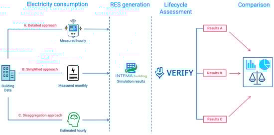
Figure 1.
An overview of the methodological framework integrating three temporal resolution pathways (A, B, C) with the VERIFY LCA/LCC tool. INTEMA provides photovoltaic generation for all cases, ensuring consistent net consumption assessment.
This design ensures that differences in environmental and economic results arise exclusively from the temporal resolution and modeling approach, rather than from variations in scope or boundary conditions. Each pathway corresponds to a distinct level of data granularity and modeling sophistication, allowing for systematic quantification of the errors introduced by temporal aggregation and by prediction error. As shown in Figure 1, all three approaches share identical system boundaries and PV generation inputs, but differ in three key aspects: (i) the temporal representation of electricity consumption, ranging from measured hourly timeseries (A) to monthly aggregated (B) and machine learning reconstructed hourly profiles (C), (ii) the treatment of electricity pricing, which is dynamic (time-of-use) in the high-resolution and reconstructed cases, and static (flat rate) in the aggregated case, and (iii) the granularity of grid emission factors.
The detailed approach (A) represents the reference baseline and establishes the upper bound of attainably accuracy by employing measured hourly electricity consumption data from sensors combined with simulated hourly photovoltaic generation profiles from INTEMA. These hourly profiles are processed within VERIFY using hourly grid emission factors and time-of-use (ToU) electricity tariffs, providing the most detailed and realistic LCA/LCC results possible with available data and serving as the benchmark for comparison.
The simplified load aggregation approach (B) corresponds to conventional practice in building-related LCA and LCC analyses. It is based on monthly electricity consumption data and monthly PV generation totals, introduced into VERIFY together with annual average grid emission factors and fixed electricity prices. Although computationally efficient, this approach neglects intra-day and seasonal variations in both demand and supply, leading to time-invariant impact estimates. The monthly aggregated configuration reflects standard building performance assessment practice, in which implementing high-resolution monitoring infrastructure, such as energy management systems, smart meters, and data-logging equipment, may be constrained by cost or technical complexity. By relying on minimal input data readily obtainable from conventional billing records, this method enables lifecycle evaluation of the majority of existing building stock lacking detailed temporal measurements, albeit at the expense of the accuracy of dynamic environmental and economic indicators.
The temporal disaggregation approach (C) which is proposed in this study illustrates a practical intermediate configuration in which only monthly consumption data are available. Here, the hierarchical temporal electricity disaggregation algorithm reconstructs hourly electricity demand profiles from monthly totals, while INTEMA supplies the corresponding hourly PV generation profile. These reconstructed series are then evaluated in VERIFY under the same hourly emission factors and ToU pricing as in the reference case (approach A).
Through these three complementary approaches, the methodology isolates and quantifies two primary error sources: (i) the temporal aggregation error (difference between approach A and B), and (ii) the prediction error produced by the disaggregation algorithm (difference between approach A and C). This enables assessment of whether the benefits of high temporal resolution outweigh the uncertainties inherent in reconstructing hourly data from coarse inputs.
The following subsections present the core methodological components in detail, including the hierarchical temporal disaggregation algorithm, the INTEMA simulation environment, and the VERIFY platform that performs LCA/LCC analysis.
2.2. Hierarchical Temporal Electricity Disaggregation Algorithm
This section introduces the proposed temporal disaggregation approach which addresses the challenge of generating hourly electricity profiles from limited input data through a structured, three-step framework that separates operational pattern extraction from temporal prediction, as presented in Figure 2. This structure allows the algorithm to identify building operational characteristics via unsupervised learning and subsequently use these patterns as constraints during the sequential disaggregation process: from monthly total consumption to allocation across the extracted operational periods, then from these monthly operational allocations to hourly prediction values. The workflow consists of data preparation and quality assurance, operational knowledge extraction via clustering, and constrained two-stage prediction. This minimal input formulation enables practical application at scale; it naturally limits the model’s ability to capture all physical and behavioral drivers of hourly load profiles. To mitigate these limitations, the clustering stage integrates operational domain knowledge that allows the model to retain essential aspects of building operation without requiring extensive metadata, while we acknowledge that incorporating richer input variables or physics-based constraints would further enhance prediction accuracy.
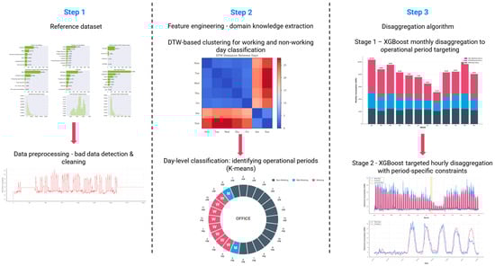
Figure 2.
Hierarchical temporal electricity disaggregation methodology. Three-step framework: (1) data preprocessing and cleaning; (2) domain knowledge extraction through DTW-based and K-means clustering, yielding six operational categories for working/non-working day periods; (3) two-stage XGBoost disaggregating monthly consumption to monthly operational period targets (Stage 1) and then monthly to hourly (Stage 2). Reference data used in Step 1 are taken from the Building Data Genome Project 2 dataset [20].
2.2.1. Step 1: Data and Preprocessing
Hourly electricity consumption data should be obtained from a comprehensive, open access building energy dataset that also includes weather variables and relevant building metadata such as floor area, occupancy type, location, and the presence of electrical HVAC systems. The selected subset should correspond to the target building typology and regional context to ensure representativeness in the modeling process. Prior to analysis, the data must undergo a structured quality control procedure to ensure completeness and reliability. Buildings with missing hourly records should be excluded to guarantee full annual coverage. Faulty sensor readings, such as negative values, extended zero-consumption periods, or constant readings indicating sensor failure, should be detected and removed. Finally, statistical outlier detection, for instance using the interquartile range method, should be applied to eliminate load profiles that deviate substantially from typical operational behavior for the building type considered. This multi-stage filtering process ensures that only high-quality, representative datasets are retained for subsequent algorithm training, validation, and temporal disaggregation analysis (step 1 in Figure 2).
2.2.2. Step 2: Feature Extraction—Operational Domain Knowledge
Operational behavior is characterized through a two-step unsupervised clustering routine applied to the training dataset. Dynamic Time Warping (DTW)-based clustering first analyzes daily consumption pattern similarity to classify days as working or non-working, capturing the fundamental operational distinction in buildings. K-means clustering is applied within each day type to identify consumption intensity patterns, segmenting the daily load curve into peak, mid-peak, and off-peak operational periods (working, mid-working, and non-working hours) (step 2 in Figure 2). Applying period segmentation to both day types maintains consistency in the hierarchical constraint framework. Working days exhibit distinct peaks during business hours, non-working days display reduced operational variation daytime hours, which may reflect weekend or holiday staff activity, whereas nighttime hours show primarily base loads from security systems and essential equipment. This dual clustering yields six operational categories, with three demand periods (peak, mid-peak, off-peak) for each day type, encoding domain knowledge about typical office building operation without requiring manual labeling or building-specific information. These operational categories constrain both stages of the hierarchical framework: stage 1 allocates monthly consumption across operational conditions, while stage 2 uses the categories both as input features and for period-specific scaling adaptation during monthly-to-hourly disaggregation.
2.2.3. Step 3: Two-Stage Hierarchical Model Architecture
In the first predictive stage, an XGBoost regression model distributes monthly electricity consumption into consumption targets for each of the six operational categories identified in step 2. For instance, monthly consumption is divided among categories such as working day peak or non-working day off-peak, producing six monthly targets for each month (one per operational category). These targets reflect operational patterns and serve as constraints for hourly prediction in stage 2 (step 3 in Figure 2).
The second stage converts these category-specific monthly targets into hourly predictions. A second XGBoost model generates hourly predictions through three mechanisms. First, it employs cumulative lag features that track electricity accumulation over rolling windows (24 h, weekly, bi-weekly, and monthly periods). These cumulative features, combined with the operational category labels from step 2, enable the model to monitor consumption progress toward the monthly operational targets established in stage 1. To prevent data leakage during testing, all cumulative features are built exclusively from the model’s own predictions with zero initialization. Second, the model uses weather variables, building characteristics (floor area, occupancy levels, and the presence of electrical HVAC systems), and operational category features as additional inputs. Third, after generating initial hourly predictions, the model applies period-specific adaptive scaling that maintains consistency between stage 1 monthly operational targets and stage 2 hourly predictions while preserving learned temporal patterns.
After generating the preliminary hourly predictions, the model applies period-specific adaptive scaling to ensure consistency between hourly and monthly energy consumption targets, or each month and operational category peak working, mid-peak working, off-peak working, peak non-working, mid-peak non-working, off-peak non-working. Let denote the stage 1 monthly consumption target, represent the set of hours in month belonging to category , and denote the initial hourly prediction for hour . The total preliminary prediction for category in month is as follows:
A category-specific scaling factor is then defined as follows:
The final scaled hourly predictions are computed as follows:
This formulation guarantees that the adjusted hourly predictions satisfy the monthly target for each operational category, i.e., . By applying separate scaling factors to each category, rather than a single uniform monthly adjustment, the model preserves intra-day temporal dynamics such as morning startup peaks, midday load dips, and evening shutdowns, while ensuring energy conservation across hierarchical levels. This adaptive scaling approach thus maintains both temporal fidelity and aggregate consistency between hourly and monthly representations.
2.3. Building Energy Performance Simulation
In this study, the INTEMA simulation environment is employed primarily to generate PV generation profiles for integration into the VERIFY LCA/LCC framework and for validation of the disaggregation algorithm (Section 3). In Section 4, where the disaggregation algorithm’s integration into the holistic LCA/LCC framework is demonstrated, INTEMA is further utilized to simulate complete building energy performance, including both thermal and electrical load estimation, thereby extending its role from data provision to comprehensive system analysis.
INTEMA is a physics-based, equation-oriented modeling environment developed in Modelica, capable of representing detailed thermodynamic and electrical interactions within building energy systems [15,16,17]. INTEMA is configured to generate hourly photovoltaic production profiles corresponding to the case study building’s geographical location, orientation, and system specifications. These outputs are subsequently aligned with the hourly or reconstructed electricity consumption profiles produced by the disaggregation model, ensuring consistent treatment of on-site generation across all evaluation approaches. This physically grounded simulation framework provides a robust foundation for quantifying self-consumption, grid exchange dynamics, and potential storage interactions within the integrated LCA/LCC assessment chain.
2.4. VERIFY—Lifecycle Assessment Platform (LCA/LCC)
VERIFY is a dynamic web-based platform for integrated lifecycle assessment and lifecycle costing from buildings to districts [18,19]. Operating within the Level(s) framework [21,22] and ISO 14040/2006 standards [23,24,25], VERIFY follows a top–down approach, decomposing performance into component-level contributions. Each system element is characterized by embodied impacts, operational efficiency, degradation patterns, and lifetime, enabling precise multi-decade tracking.
VERIFY integrates with external energy tools to process spatially and temporally resolved flows. The platform receives hourly energy profiles from INTEMA.building or ML disaggregation algorithms, converting operational consumption into environmental impacts using time-varying emission factors at the component level. Time-dependent energy and emission factors ensure that hourly grid carbon intensity and electricity price fluctuations directly influence the results.
Environmental and economic indicators are calculated in parallel, maintaining internal coherence. Key metrics include lifecycle global warming potential, primary energy demand, carbon savings, lifecycle cost, net present value, and payback period within Level(s) requirements. For this study, VERIFY processes three approaches (measured hourly data, measured monthly, disaggregated hourly), with hourly grid carbon intensity and time-of-use pricing used to compute 25-year outcomes, evaluating how temporal resolution affects assessment accuracy.
3. Validation of the Proposed Approach
To demonstrate the impact of temporal resolution on building LCA and LCC results, the three evaluation approaches described in Section 2 are applied to the same office building case study under identical system boundaries. This design ensures that any variation in environmental and economic indicators arises solely from the temporal granularity and modeling approach, rather than from discrepancies in scope or assumptions. Each pathway thus represents a different level of data detail and modeling sophistication, allowing for systematic quantification of the errors introduced by temporal aggregation and prediction error.
3.1. System Definition
3.1.1. Building Modeling
The selected building is a two-story office building in Cardiff, UK, with a total floor area of 1805 m2 and one year of measured hourly electricity consumption data from building sensors. This building data were sourced from the Building Data Genome Project 2 dataset [20] but were explicitly excluded from the training phase of the hierarchical temporal disaggregation algorithm to ensure an unbiased evaluation of predictive performance. The building is equipped with a natural gas boiler for space heating; however, this study focuses exclusively on electricity consumption to isolate the effects of temporal resolution on grid emission factors and ToU electricity pricing, which exhibit strong hourly variability. Natural gas use is excluded from the analysis, as its carbon intensity profile remains relatively stable over time, as commonly assumed in building LCA practices, so its lifecycle impact does not change with temporal resolution. Including it would add complexity without affecting the results and would obscure the specific influence of hourly electricity grid variation. Thus, our findings apply directly to the electricity share of building energy use, while gas-related impacts remain unchanged across temporal resolutions.
For demonstration purposes, the building is assumed to host a hypothetical 30 kWp rooftop PV system covering 150 m2, mounted at a 35° tilt facing due south (180° azimuth). This configuration represents a typical setup for office buildings at the given latitude. The system includes embodied impacts associated with manufacturing and installation (17,700 kg CO2-eq; 217 GJ primary energy) and end-of-life treatment (354 kg CO2-eq; 3.3 GJ primary energy) and is assigned an operational lifetime of 25 years. A representative capital cost of GBP 24,000 is assumed to enable economic performance indicators such as payback period, thereby linking temporal resolution not only to environmental metrics but also to financial performance.
PV generation is simulated with the INTEMA energy system simulation tool, providing hourly profiles for a full year based on Cardiff’s climatic conditions and the specified system parameters. Including PV generation in the case study introduces the critical issue of temporal alignment between on-site generation and consumption: whereas monthly aggregation obscures these dynamics, hourly resolution reveals the interplay between daytime production peaks, evening demand peaks, and the differential economic value of self-consumed versus exported electricity.
3.1.2. Electricity Pricing Schemes
To evaluate the economic implications of temporal resolution in building energy assessment, pricing schemes are aligned to each approach’s data granularity. Users with hourly resolved datasets (approaches A and C) employ dynamic ToU tariffs, while users relying on monthly aggregated data (approach B) apply an average flat rate. This contrast illustrates how temporal aggregation constrains the ability to capture cost variations throughout the day and across seasons.
ToU pricing for hourly approaches: For the high-resolution and reconstructed cases, ToU electricity tariffs are derived from official UK non-domestic electricity statistics and realistic time-band structures. The base price of 32.6 p/kWh (excluding VAT but including all other charges) is taken from the UK Government’s Quarterly Energy Prices publication [26] and distributed across three daily bands following the National Grid Electricity Distribution (South Wales) distribution use of system (DUoS) schedule for low-voltage (LV) site-specific customers [27]. The resulting tariffs comprise the following:
- Peak period applies from 17:00 to 19:30 (2.5 h/day) with import rates of 47.5 p/kWh;
- Mid-peak period applies from 07:30 to 17:00 and 19:30 to 22:00 (12 h/day) at 36.9 p/kWh;
- Off-peak period applies for all remaining hours (9.5 h/day) at 23.2 p/kWh.
- These rates are calibrated such that their consumption-weighted average equals the official non-domestic electricity price, maintaining consistency with actual UK commercial electricity costs while reflecting realistic temporal price variability. These ToU rates enable precise economic assessment by matching hourly consumption and generation patterns with corresponding time-dependent electricity prices.
Flat-rate pricing for monthly aggregated approach: For the static resolution case (approach B), a uniform import price of 32.6 p/kWh is applied, representing the official average non-domestic tariff (excluding VAT, including all charges). This flat rate reflects the limitation that users with only monthly aggregated consumption data cannot differentiate when electricity was consumed within the billing period and must apply a uniform price to all consumption cases. Mathematically, this rate equals the consumption-weighted average of the ToU structure:
where = 2.5 h/day, = 12 h/day, = 9.5 h/day, and = 24 h/day, yielding = 32.6 p/kWh. This pricing approach represents realistic practice where monthly billing precludes time-differentiated economic assessment, demonstrating the economic penalty of temporal aggregation even when total energy quantities are identical.
Electricity exported from the on-site PV system is assumed to receive a fixed price of 10 p/kWh in all cases, applied uniformly across all hours or billing periods.
3.1.3. Grid Carbon Intensity and Primary Energy Factors
Environmental assessment parameters are selected to match each approach’s temporal scope. Hourly grid carbon intensity data for the UK in 2024 are obtained from Electricity Maps [28], with values ranging from 0.008 to 0.278 kg CO2-eq/kWh during periods of high renewable penetration and fossil-dominated peak demand, respectively. These hourly values are applied in the hourly resolved approaches (A and C). For the monthly aggregated approach (B), the annual average grid carbon intensity of 0.225 kg CO2-eq/kWh is sourced from the Annual Official 2024 Greenhouse Gas Reporting Conversion Factors published by the UK Government [29]. This represents the official UK electricity generation emission factor for 2024, ensuring regulatory compliance and comparability with standard reporting frameworks.
Primary energy factors follow the UK Government’s standardized methodology [30]. Grid electricity is assigned a primary energy factor of 1.969, while on-site PV generation is taken as 1.0. These factors ensure comparability between approaches.
3.1.4. Overview of Assessment Parameters
Table 1 summarizes the main parameters adopted across all three approaches, including temporal resolution, environmental factors, and economic assumptions.

Table 1.
Assessment parameters for three evaluation approaches.
3.1.5. Input Timeseries Data
The three evaluation pathways described in Section 2 are now applied to the Cardiff office building introduced in Section 3.1. Each pathway shares identical system boundaries and PV generation data, differing in the temporal resolution of grid emission inputs, pricing, and electricity consumption. This configuration isolates the effect of temporal granularity on the accuracy of LCA and LCC outcomes. Approach A represents the ideal reference scenario in which complete hourly measured electricity consumption data are available from building monitoring systems and therefore utilizes available hourly timeseries data. It serves as the reference baseline against which approach B (monthly aggregation) and approach C (hourly disaggregation) are evaluated. Approach B represents a practical intermediate configuration, more detailed than annual aggregation yet considerably less data-intensive than hourly monitoring. It is typical for buildings that rely on standard utility billing in the absence of smart-metering infrastructure. Operating exclusively with monthly aggregated data, the method applies annual average grid emission factors and flat-rate electricity pricing, thereby removing temporal resolution from both energy flows and grid characteristics.
Hourly electricity consumption data from the building’s energy monitoring system are plotted in Figure 3a, where distinct seasonal operational patterns between January and July are shown. January exhibits higher energy demand with daily peak loads reaching approximately 50 kWh during working hours, characteristic of reduced daylight availability, and full occupancy patterns. July displays lower overall consumption with peak values around 27 kWh, reflecting increased natural daylight, and the influence of summer vacation schedules that decrease occupancy. The clear contrast between working and non-working days visible in both months highlights the characteristic operational rhythm of an office building, with pronounced weekday peaks and weekend minima.
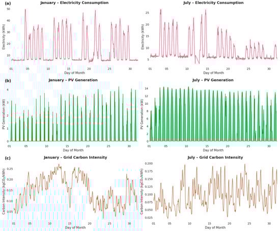
Figure 3.
Hourly temporal patterns of the following available timeseries data for January and July: (a) electricity consumption, (b) PV generation, and (c) grid carbon intensity.
Hourly photovoltaic generation is simulated using the INTEMA physics-based model and Figure 3b illustrates the seasonal variation in PV output between January and July. January shows limited generation due to shorter daylight hours, lower solar angle, and reduced irradiance, with greater daily variability reflecting winter cloud cover and weather instability. July demonstrates substantially higher and more consistent output, with daily peaks frequently reaching around 15 kW and regular curve generation patterns throughout the month. The seasonal pattern shows an inverse relationship between PV generation and building consumption.
Hourly grid carbon intensity data for the UK in 2024 were obtained from Electricity Maps [28], ranging from 0.008 kg CO2-eq/kWh during periods of high renewable penetration to 0.278 kg CO2-eq/kWh during fossil fuel-dominated peak demand periods. Figure 3c presents hourly carbon intensity for January and July, demonstrating both temporal and seasonal variations. Electricity pricing data follow the ToU tariff structure described in Section 3.1.2, with rates ranging from 23.2 p/kWh during off-peak periods to 47.5 p/kWh during peak hours.
Together, these hourly datasets for consumption, PV generation, grid emission factors, and electricity tariffs constitute the most detailed temporal representation available and form the reference baseline for evaluating the accuracy and practical implications of the two alternative approaches.
Figure 4 presents monthly electricity consumption totals for the complete year, yielding 12 data points representing aggregate energy use per billing period (total annual consumption: 98.8 MWh). In this study, monthly values are obtained by aggregating hourly measured data; however, in typical applications, these values would be sourced directly from standard utility billing records. Monthly PV generation totals from the INTEMA simulations are similarly aggregated to 12 monthly values, with a total annual generation of 22.2 MWh. These monthly aggregates capture seasonal variations, higher consumption during winter months with reduced daylight and full occupancy (January: 10.3 MWh) and lower consumption during summer with increased natural daylight and vacation schedules (August: 5.2 MWh), but eliminate all intra-month temporal information regarding daily operational patterns, peak demand periods, and hour-to-hour fluctuations in both building loads and renewable generation.
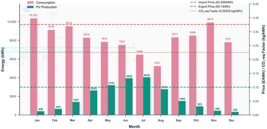
Figure 4.
Monthly electricity consumption and PV generation, with flat-rate import/export prices and annual grid carbon intensity.
Approach B applies constant annual emission factors, eliminating temporal variability in grid emissions from changing generation mix and seasonal patterns. It also uses flat-rate electricity pricing, equivalent to the consumption-weighted average of the time-of-use tariff, removing temporal price signals. This uniform approach treats all electricity as economically identical regardless of timing, eliminating the financial incentives for load shifting and peak reduction that exist under time-differentiated pricing.
3.2. Disaggregation Algorithm Results
Hourly electricity consumption profiles are generated using the developed hierarchical temporal disaggregation algorithm, which reconstructs 8760 hourly values from monthly aggregated electricity data, as can be seen in Figure 5, in conjunction with building metadata (office type, 1805 m2 floor area, occupancy levels) and hourly weather data for Cardiff. The algorithm applies domain knowledge about typical office operation, distinguishing working and non-working days as well as operational periods within each day. Monthly totals are first disaggregated into daily patterns and then into hourly profiles, with scaling applied at the operational-period level to ensure that monthly energy use exactly matches monthly aggregated data.
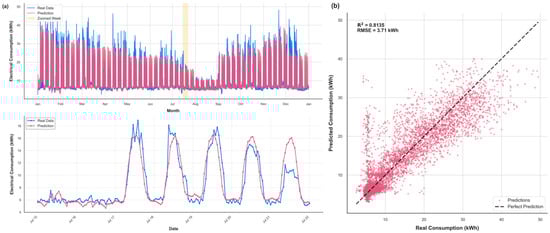
Figure 5.
Hierarchical disaggregation algorithm validation results. (a) Annual and summer period comparison between measured and predicted hourly electricity consumption, showing successful capture of seasonal, monthly, and daily operational patterns. (b) Hourly prediction accuracy scatter plot (R2 = 0.813, RMSE = 3.71 kWh).
The algorithm’s performance is evaluated by comparing predicted hourly profiles against measured electricity consumption from building sensors over the entire yearly period. Figure 5a demonstrates that the algorithm successfully reproduces both seasonal and intra-month variations, with predicted values (red) closely following the measured consumption values (blue). Figure 5a highlights the summer period, illustrating that daily operational patterns, such as working day peaks and weekend reductions, are accurately captured. Figure 5b presents the scatter plot of predicted versus measured hourly consumption, yielding R2 = 0.813 and RMSE = 3.71 kWh. The prediction error for the Cardiff building is applied to subsequent environmental and economic analyses.
All other parameters are identical to those used in the reference baseline (approach A), including the simulated PV generation profiles, electricity pricing schemes, and grid emission factors. The only difference between approaches lies in the predicted electricity consumption data, ensuring direct comparability of results.
To ensure that the performance observed for the Cardiff building is representative rather than case-specific, the hierarchical disaggregation algorithm was additionally validated across the entire (filtered) office building subset of the Building Data Genome Project 2, spanning multiple UK regions with differing weather conditions and operational characteristics. Using cross-validation at the building level (Figure 6), the model achieved a mean absolute error (MAE) of 2.75 ± 0.83 kWh, a root-mean-square error (RMSE) of 3.80 ± 1.04 kWh, and a mean absolute percentage error (MAPE) of 19.61 ± 5.50%. The corresponding 95% confidence intervals, [1.98, 3.52] kWh for MAE, [2.84, 4.77] kWh for RMSE, and [14.53, 24.70]% for MAPE, indicate stable predictive accuracy across office buildings located in different UK climatic contexts and exhibiting diverse operational profiles. This process serves as an independent validation test for the detailed LCA/LCC comparison presented in Section 2.1. The cross-validation results also place the model’s performance within the range of existing monthly-to-hourly reconstruction methods, showing that it matches or exceeds other approaches that rely on similarly limited monthly inputs, while recognizing that methods requiring richer, high-resolution data achieve higher accuracy but cannot be applied under typical real-world data scarcity; in this context, the contribution of the present work lies in enabling reliable hourly reconstruction in exactly those situations where high-input methods cannot operate.
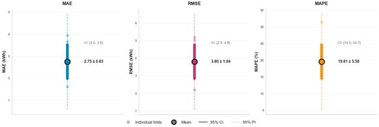
Figure 6.
Cross-validated error metrics (MAE, RMSE, MAPE) for hierarchical disaggregation algorithm across UK office buildings.
3.3. Environmental and Economic Performance
3.3.1. Detailed Results per Approach
The 25-year LCA for approach A (reference case) indicates total greenhouse gas (GHG) emissions of 317.1 tons CO2-eq (12.7 tons CO2-eq/year, 3.5 kg CO2-eq/m2/year). Embodied emissions from photovoltaic system manufacturing and installation contribute 17.7 tons CO2-eq in year one, while operational emissions total 299.4 tons CO2-eq over the building’s lifetime. The PV system delivers 78.3 tons CO2-eq of avoided emissions through on-site renewable generation, 71.4 tons from self-consumed electricity and 6.9 tons from grid-exported surplus, representing a 19.8% reduction in lifecycle emissions relative to grid-only operation (395.5 tons CO2-eq). Cumulative primary energy demand reaches 4724 GJ over 25 years (189 GJ/year), with operational energy accounting for 98.7% of total demand. The building achieves 19.3% renewable energy self-sustenance, with 91.1% of PV generation consumed on site, indicating effective temporal matching between generation availability and load patterns. From an economic perspective, total lifecycle costs amount to GBP 448,366 over 25 years (17,935 GBP/year, 4.97 GBP/m2/year). PV system capital expenditure of GBP 24,000 represents 5.4% of lifecycle costs, with operational electricity purchases comprising the remaining 94.6%. The PV investment demonstrates economic viability with a 3.1-year payback period and net present value of GBP 97,392 at a 4% discount rate, driven by the value differential between self-consumed grid electricity (23.2–47.5 p/kWh ToU rates) and export compensation (10 p/kWh). The levelized cost of PV-generated electricity is 7.0 p/kWh, considerably lower than the grid import price.
The 25-year LCA for approach B yields total GHG emissions of 456.9 tons CO2-eq (18.3 tons CO2-eq/year, 5.1 kg CO2-eq/m2/year). Embodied emissions from the photovoltaic system contribute 17.7 tons CO2-eq in year one, while operational emissions total 439.2 tons CO2-eq over the building’s lifetime. The method reports 117.7 tons CO2-eq of avoided emissions from PV self-consumption and assigns zero emissions savings to grid exports. Cumulative primary energy demand reaches 4673 GJ over 25 years (186.9 GJ/year, 51.8 GJ/m2/year). The building achieves 21.1% renewable energy self-sustenance, with the model calculating 100% PV self-consumption as a mathematical consequence of monthly aggregation methodology. Economically, total lifecycle costs amount to GBP 435,499 over 25 years (17,420 GBP/year, 4.83 GBP/m2/year). PV system capital expenditure of GBP 24,000 represents 5.5% of lifecycle costs, with operational electricity purchases comprising the remaining 94.5%. The flat-rate electricity pricing of 32.6 p/kWh for imports and 10 p/kWh for exports is applied uniformly to all energy flows regardless of timing. The PV investment shows a 3.5-year payback period and net present value of GBP 83,478 at a 4% discount rate. Under the monthly aggregation approach, all PV generation is credited as displacing flat-rate grid purchases (32.6 p/kWh), as the methodology cannot distinguish between self-consumed electricity and grid exports within monthly billing periods. Annual present-value operational costs decline from GBP 24,979 in year 1 to GBP 10,064 in year 25, reflecting that the discount rate applied reduces the present value of future costs.
The 25-year LCA for approach C produces total greenhouse gas emissions of 315.5 tons CO2-eq (12.6 tons CO2-eq/year, 3.5 kg CO2-eq/m2/year). Embodied emissions from the photovoltaic system contribute 17.7 tons CO2-eq in year one. Operational emissions total 297.8 tons CO2-eq over the building’s lifetime. The PV system delivers 78.3 tons CO2-eq of avoided emissions through on-site renewable generation: 73.0 tons from self-consumed electricity and 5.3 tons from grid-exported surplus. Cumulative primary energy demand reaches 4713 GJ over 25 years (188.5 GJ/year, 52.2 GJ/m2/year). The building achieves 19.7% renewable energy self-sustenance, with 93.2% of PV generation consumed on site and the remaining 6.8% exported to the grid. Total lifecycle costs amount to GBP 446,304 over 25 years (17,852 GBP/year, 4.95 GBP/m2/year). PV system capital expenditure of GBP 24,000 represents 5.4% of lifecycle costs, with operational electricity purchases comprising the remaining 94.6%. The PV investment shows a 3.1-year payback period and net present value of GBP 97,392 at a 4% discount rate. The time-of-use electricity pricing structure (peak: 47.5 p/kWh, mid-peak: 36.9 p/kWh, off-peak: 23.2 p/kWh, export: 10 p/kWh) is applied to the ML-predicted hourly consumption profiles. The levelized cost of PV-generated energy is 7.0 p/kWh. Annual present-value operational costs decline from GBP 25,599 in year 1 to GBP 10,348 in year 25, reflecting that the discount rate applied reduces the present value of future costs, with PV-avoided grid purchases providing additional savings throughout the assessment period. The complete environmental and economic performance metrics for approach C, demonstrate the outcomes of the disaggregation approach utilizing predicted hourly consumption profiles.
3.3.2. Comparative Discussion
This section evaluates the three LCA approaches by comparing their environmental and economic outcomes, analyzing the sources and magnitudes of deviations from the reference baseline (approach A), and examining the practical implications for building performance assessment and renewable energy integration studies.
Table 2 and Figure 7 present a comprehensive comparison of environmental metrics across all three approaches, with deviations calculated relative to approach A as the reference baseline.
Table 2.
Environmental performance comparison across approaches.
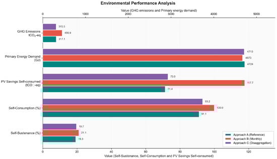
Figure 7.
Environmental performance comparison across three approaches (25-year lifecycle). Approach B (monthly, red) overestimates GHG emissions by 44.1% (456.9 vs. 317.1 tons CO2-eq) and PV savings by 64.8% (117.7 vs. 71.4 tons). Approach C (disaggregation, purple) achieves 0.5% GHG accuracy and 2.2% PV savings deviation from approach A (hourly baseline, teal). Primary energy shows minimal sensitivity (1.1% range) across approaches.
Approach B overestimates lifecycle emissions by 44.1% (139.8 tons CO2-eq). The annual average grid carbon factor (0.225 kg CO2-eq/kWh) weights all hours equally. The 100% self-consumption assumption inflates PV carbon savings by 50.3% by crediting all generation at the annual average factor while eliminating recognition of actual exports (8.9% of generation) that receive lower carbon credit.
Approach C achieves 0.5% accuracy (1.6 tons deviation) despite using monthly aggregated input data. The hierarchical algorithm preserves temporal consumption patterns that align with time-varying grid carbon intensity. Incorporating operational domain knowledge (working/non-working days, operational periods) produces daytime-concentrated profiles matching actual consumption timing, while monthly scaling ensures cumulative accuracy. The 2.1-percentage-point self-consumption overestimation (93.2% vs. 91.1%) reflects consumption smoothing that marginally improves PV alignment.
Primary energy demand in Approach B is 1.1% lower than the reference because the 100% self-consumption assumption treats more PV generation as directly displacing grid electricity (with transmission losses) rather than being exported. Approach C shows minimal deviation (−0.2%) as the predicted 93.2% self-consumption closely matches the measured 91.1%.
Table 3 and Figure 8 present comprehensive economic metrics across all three approaches, revealing how temporal resolution and pricing structures interact to affect financial assessment accuracy.
Table 3.
Economic performance comparison across approaches.
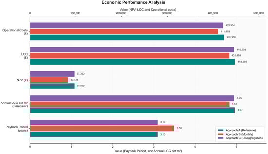
Figure 8.
Economic performance comparison across three approaches. Approach B (monthly, red) underestimates lifecycle costs by 2.9% (GBP 435,499 vs. GBP 448,366) and PV net present value by 14.3% (GBP 83,478 vs. GBP 97,392) with extended payback period (+12.9%, 3.5 vs. 3.1 years).
Approach B underestimates lifecycle costs by 2.9% (£12,867) and produces a GBP 13,914 lower PV net present value with 0.4-year extended payback compared to the measured reality. These errors stem from flat-rate pricing that misrepresents both baseline electricity costs and PV savings.
The flat rate of 32.6 p/kWh represents a generic consumption-weighted average: (2.5 h × 47.5 p/kWh + 12 h × 36.9 p/kWh + 9.5 h × 23.2 p/kWh)/24 h. However, this office building concentrates consumption during working hours (07:30–17:00) when mid-peak rates apply (36.9 p/kWh), with minimal overnight off-peak usage (23.2 p/kWh) and limited evening peak consumption (47.5 p/kWh). The building’s actual time-weighted electricity cost approaches 36.9 p/kWh, exceeding the 32.6 p/kWh flat rate and producing systematic cost underestimation.
This baseline underestimation extends to PV economic assessment through the 100% self-consumption assumption. Approach B calculates all generation (20.9 MWh/year) as avoiding purchases at 32.6 p/kWh. The reality differs: approaches A and C show 91–93% self-consumption with savings varying by timing (peak: 47.5 p/kWh, mid-peak: 36.9 p/kWh, off-peak: 23.2 p/kWh), with 7–9% exports at 10 p/kWh. Since this office building’s daytime PV generation predominantly offsets mid-peak consumption at 36.9 p/kWh, the actual savings per self-consumed kWh exceeds the 32.6 p/kWh flat-rate assumption. Crediting PV savings at the lower flat rate while also underestimating baseline costs produces a compounding effect: Approach B calculates PV as saving less money (32.6 p/kWh) from a baseline that already costs less (32.6 p/kWh average vs. actual 36.9 p/kWh). The result is a net present value GBP 13,914 lower than that of the PV investment under time-of-use pricing (Figure 9).
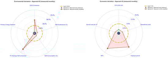
Figure 9.
Deviation of monthly aggregation approach B from baseline (approach A). Left: Environmental metrics show systematic overestimation (GHG +44.1%, self-consumption +8.9%, PV savings +64.8%). Right: Economic metrics exhibit mixed deviations (lifecycle costs −2.9%, payback +12.9%, NPV −14.3%). Orange dashed circles indicate average deviation magnitude (26.8% environmental, 7.2% economic).
Approach C shows 0.5% lifecycle cost deviation (GBP 2062 over 25 years) but achieves exact PV economic equivalence with approach A: identical payback (3.1 years) and identical NPV (GBP 97,392). This PV equivalence, despite the moderate hourly prediction accuracy (R2 = 0.813, RMSE = 3.71 kWh), results from the monthly reconciliation mechanism [32]. Under monthly reconciled net-metering, PV savings depend on the balance between self-consumed generation (displacing purchases at ToU rates) and exported generation (earning 10 p/kWh credits that offset imports within the monthly cycle). The hierarchical algorithm’s monthly scaling and preserved operational patterns produce nearly identical self-consumption rates (93.2% vs. 91.1%), yielding the same monthly PV savings through equivalent combinations of direct displacement and export credit offsets. The small lifecycle cost deviation stems from differences in electricity procurement costs unrelated to PV performance: predicted consumption patterns slightly differ from actual patterns in their alignment with ToU tariff periods, producing minor variations in baseline electricity costs across 300 monthly billing cycles, while PV economic benefits remain identical (Figure 10).
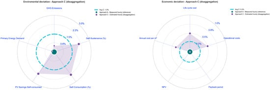
Figure 10.
Environmental and economic deviations of approach C from baseline (approach A). Disaggregation algorithm achieves minimal environmental deviation (avg. 1.5%) and near-zero economic deviation (avg. 0.3%).
The LCOE remains identical (7.0 p/kWh) across all approaches because it depends only on PV system costs and generation quantity, independent of temporal consumption patterns or assessment methodology.
3.3.3. Methodological Insights
This comparative analysis reveals four fundamental principles for building LCA accuracy. First, preserving hourly patterns outweighs measurement precision. Approach C with predicted profiles (R2 = 0.813) achieves 0.5% environmental error, while approach B with exact monthly totals produces 44.1% error (139.8 tons CO2-eq). Using identical monthly input data, the 43.6% accuracy improvement demonstrates that capturing consumption timing relative to grid carbon intensity variations matters more than aggregate quantity precision. This finding challenges monitoring strategies prioritizing high-precision monthly metering over lower-precision hourly data.
Second, annual average emission factors systematically misestimate emissions for buildings with daytime-concentrated operations. This office building operates predominantly during daytime hours when grid carbon intensity differs from the 24 h average. Applying the annual factor (0.225 kg CO2-eq/kWh) inappropriately weights nighttime periods when the building consumes minimal energy.
Third, primary energy sensitivity to temporal resolution depends on the variability in the underlying factors. Although grid primary energy factors are constant in this study, differences in PV self-consumption still affect the building’s overall energy mix. PV generation carries a primary energy factor of 1.0, whereas grid electricity carries 1.969, so the different self-consumption rates obtained under the three approaches (91.1%, 100.0%, and 93.2%) lead to small shifts in the balance between on-site and grid electricity. These effects are modest in this case but would be considerably larger in buildings with storage or vehicle-to-building systems, where hourly charging and discharging behavior introduces stronger temporal variations into the energy mix.
Fourth, the identical PV economic outcomes for approaches A and C result from the monthly net-metering structure combined with the relatively small prediction errors of the disaggregation model. Although the two approaches differ in hourly self-consumption and export patterns, these differences are modest and do not substantially alter the monthly net import–export balances within each tariff period, which determine PV savings under the applied tariff scheme. Because PV generation is identical across approaches and the reconstructed profiles preserve similar period-level energy balances, the resulting PV-related economic indicators coincide. This does not imply that hourly fidelity is unimportant for LCC; under tariff structures without monthly netting, or in cases where prediction errors shift energy between tariff periods with different prices, economic outcomes would diverge. Even within monthly reconciliation, larger temporal inaccuracies would affect PV savings and total lifecycle costs.
An additional observation is that, across all approaches, economic deviations remain smaller than environmental ones. This behavior arises from the structure of electricity pricing, which varies across fixed tariff periods rather than individual hours and remains consistent throughout the year. As a result, minor temporal mismatches in consumption exert limited influence on cost estimation. Combined with the reconciliation mechanism, where exported electricity is credited back within each billing cycle, this structure effectively reproduces the self-consumption equivalence observed under high-resolution monitoring [32]. Hence, the economic results across all three approaches show much closer agreement compared to their environmental counterparts.
4. Application Case Study: Massagno District in Switzerland
4.1. District System Definition
Building on the disaggregation model validated in Section 3 and the methodological components introduced in Section 2, this section applies the hybrid LCA/LCC workflow to the Massagno district. The objective is to demonstrate how the integrated framework can be applied in a district-scale context, represented by the Massagno local energy community in Switzerland, under realistic conditions of heterogeneous data availability. The disaggregation algorithm was trained exclusively on UK office buildings, and its application to the Swiss office building is performed under the practical assumption of broadly similar operational and climatic conditions. This is a simplifying assumption used solely to enable the demonstration, and it does not represent a validated or recommended transfer of the model to a new climate. Applying the disaggregation method to different climates or typologies would require retraining on appropriate datasets. Within this configuration, the disaggregation model and INTEMA process their respective data streams independently. The disaggregation algorithm reconstructs hourly electricity demand for the office building from monthly data, while INTEMA generates physics-based thermal profiles for that same office building as well as complete energy profiles for all remaining buildings. These separate outputs are then combined within VERIFY to produce a unified district-level environmental assessment. This case reflects real deployment conditions in which data coverage and measurement granularity vary significantly across buildings, and serves solely to demonstrate how the hybrid workflow can be applied in practice, rather than to validate model performance, since no actual hourly measurements are available for comparison.
The Massagno district comprises eight buildings with diverse typologies across residential, commercial, and institutional sectors, totaling 11,590 m2 of conditioned floor area. The district is located in Switzerland at 46.01° N, 8.94° E, and an elevation of 355 m. Hourly building energy simulations are performed using Swiss typical meteorological year climate data combined with building-specific geometric and physical specifications.
The dataset available for analysis includes building geometry, physical system characteristics, and equipment inventories, as well as monthly electricity billing for one building and annual totals for the others. These represent typical data constraints encountered in district-scale studies, where smart-meter coverage is incomplete. Accordingly, the analysis focuses exclusively on environmental performance over a 20-year period (2022–2041). Economic parameters, such as capital costs, maintenance expenditures, fuel prices, and electricity tariffs, were unavailable, and therefore, no financial evaluation is included. The environmental assessment primarily demonstrates the framework’s capability to integrate multi-resolution datasets and align them with hourly grid emission factors across a complex multi-building system.
The district contains the following:
- A 4695 m2 dormitory (939 m2 per floor across 5 floors) serving residential institutional functions with oil boiler heating (510 kW total capacity), air conditioning (79 kW), hot water storage (1500 L), and the district’s only renewable generation system, a 59.4 kWp photovoltaic system (297 m2 array). Annual electricity consumption is 1549 MWh.
- A 2232 m2 warehouse (744 m2 per floor, 3 floors) providing commercial storage with electric resistance heating (60 kW) and hot water storage (50 L). Annual consumption is 737 MWh.
- A 1345 m2 office building (269 m2 per floor, 5 floors) operating with natural gas boiler heating (140 kW), water chiller cooling (20 kW, 2 units, COP 4.0), and hot water storage (400 L). Annual consumption is 442 MWh.
- Five residential buildings ranging from 276 to 1722 m2 total area (two to six floors, 127–287 m2 per floor) equipped with oil boiler heating (30–40 kW) and 200–400 L hot water storage, with annual consumption ranging from 92 to 568 MWh.
District infrastructure includes a 630 kVA transformer and three public EV charging stations, one DC fast charger (10 kW) and two AC chargers (11 kW each), with estimated annual consumption of 2500 kWh per charger. Total district annual electricity consumption is 3916 MWh.
The case study demonstrates the application of the hybrid LCA framework under realistic data constraints, where high-resolution (hourly) monitoring is not uniformly available. Two complementary modeling strategies were employed depending on data availability:
- Machine learning disaggregation: The office building (Building 3) applied the hierarchical temporal disaggregation to monthly data (12 monthly values), processing monthly totals with building metadata (office typology, 1345 m2 total conditioned area), occupancy levels, and weather data to generate 8760 hourly predictions annually.
- Physics-based simulation: INTEMA generates the physics-based thermal load for the same office building (Building 3) and produces the complete hourly energy profiles for the remaining buildings, including the dormitory (Building 1), warehouse (Building 2), and residential buildings (Buildings 4–8). The simulations are calibrated to reproduce reported annual consumption totals and are based on building-specific characteristics, including occupancy, envelope parameters, geometry, and operational behavior.
Thermal energy demand for heating and cooling was simulated for all buildings, since no fuel consumption data were available. INTEMA produced hourly loads using building geometry, envelope characteristics, temperature setpoints, and climate data. Oil consumption for boilers and electricity consumption for air conditioning were calculated based on simulated hourly thermal loads and equipment efficiencies. PV generation for the dormitory’s rooftop installation was also simulated using climate data and system specifications, providing hourly temporally resolved generation profiles for self-consumption assessment.
Asset degradation modeled hourly performance decline across the 20-year period. Consumption equipment efficiency degrades progressively, increasing energy demand over time, while the photovoltaic system experiences generation output reduction following typical module aging characteristics. District infrastructure including EV charging stations and transformers were treated as annual average consumption without hourly temporal disaggregation, isolating application of the hybrid methodology specifically to the building sector while maintaining overall district energy accounting.
Environmental impact assessment incorporated hourly Swiss grid carbon intensity data for 2022–2024 obtained from Electricity Maps. For projection years (2025–2041), the 2024 hourly emission factor profile was repeated to preserve temporal resolution while acknowledging uncertainty regarding future grid decarbonization trajectories. The assessment quantified operational electricity and fuel consumption, on-site renewable generation and self-consumption, grid interaction, and embodied emissions from installed systems over the 20-year lifecycle.
4.2. Results and Discussion
The environmental performance of the Massagno district was evaluated over a 20-year horizon (2022–2041) using the integrated hybrid framework. The results are summarized in Table 4, which reports annual and cumulative performance indicators for each building and for the district. The analysis reflects the diversity of building typologies within the district and illustrates the resulting environmental performance under heterogeneous data availability.
Table 4.
Massagno district environmental performance summary.
At a district scale, the 20-year LCA yields total GHG emissions of 9429 tons CO2-eq, equivalent to 472 tons CO2-eq annually. The building sector accounts for 9419 tons, while district infrastructure contributes 10 tons. Total primary energy demand reaches 226,227 megawatt-hours over 20 years (11,311 MWh annually), with the building sector consuming 225.8 GWh (11.3 GWh/year) and infrastructure contributing 414 MWh.
The dormitory emerges as the most energy-intensive building, responsible for 4358 tons over 20 years (218 tons/year). Despite high absolute emissions, the building achieves 46.4 kg/m2/year carbon intensity, reflecting the dilution effect of the large conditioned floor area. Primary energy demand reaches 91,605 MWh over 20 years (4580 MWh/year, 976 kWh/m2/year). The building’s rooftop system comprises a 59.4 kWp capacity and produces 895 MWh across the assessment period (44.8 MWh/year), achieving 100% self-consumption because its generation consistently remains below demand. Complete self-consumption yields 10.4 tons CO2-eq avoided emissions and yields a self-sustenance level of 2.9%, corresponding to 1.2% of total district consumption. These results demonstrate PV’s potential to decouple carbon intensity from absolute consumption; despite consuming substantially more than all other buildings, its carbon intensity of 46.4 kg/m2/year remains lower than four of five residential buildings (73.2, 73.0, 71.0, and 105.0 kg/m2/year for Buildings 4, 6, 7, and 8, respectively).
The office building (1345 m2), where the hierarchical temporal disaggregation was applied to reconstruct hourly electricity consumption profiles and where INTEMA was used to generate physics-based thermal load, illustrates how the hybrid workflow operates within the district context. The building achieves 35.2 kg/m2/year carbon intensity, generating 948 tons over 20 years from 442 MWh annual consumption. Primary energy totals 26,414 MWh (1321 MWh/year, 982 kWh/m2/year).
The warehouse (2232 m2) demonstrates the lowest carbon intensity at 6.1 kg/m2/year despite substantial annual consumption of 737 MWh, generating only 271 tons over 20 years. This outcome reflects the predominance of electric resistance heating, which, while energy-intensive, benefits from Switzerland’s relatively low-carbon electricity mix compared with direct fossil fuel combustion. Primary energy totals 38,884 MWh over 20 years (1944 MWh/year, 871 kWh/m2/year).
The five residential buildings exhibit carbon intensities ranging from 39.2 kg/m2/year (Building 5, 1722 m2) to 105.0 kg/m2/year (Building 8, 276 m2). This variation reveals the influence of building scale and thermal envelope effects: smaller dwellings exhibit higher relative heat losses and lower equipment efficiency due to surface-to-volume ratios and part-load operation. Corresponding primary energy intensities vary between 965 and 1199 kWh/m2/year, mirroring the same inverse relationship with floor area.
An overview of the results is presented in Figure 11.
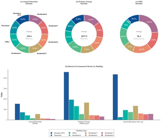
Figure 11.
District-scale results for Massagno energy community (8 buildings, 20-year horizon). Top: Distribution of (a) electricity (avg. 330.4 kWh/m2/year), (b) primary energy (avg. 1037.9 kWh/m2/year), and (c) GHG intensity (avg. 56.1 kgCO2-eq/m2/year) by building type. Bottom (d): Absolute metrics showing that dormitory and warehouse dominate consumption.
Temporal analysis of operational emissions reveals year-to-year variability driven by changes in grid carbon intensity and progressive degradation of building assets. Year one reaches 502 tons CO2-eq (2022 actual grid factors), while years two and three show 504 and 453 tons (2023–2024 measured factors). Years four through seven stabilize around 455–461 tons as the 2024 profile repeats, while years eight and nine exhibit elevated emissions of 465 and 467 tons. This upward trend reflects the combined effect of equipment efficiency degradation, increasing electricity and fuel consumption to maintain service levels, and photovoltaic generation decline due to module aging, alongside seasonal peaks within the recycled hourly emission factor profile. The temporal variability illustrates the importance of preserving hourly resolution, as annual average emission factors would obscure these interactions between time-varying grid carbon intensity, weather-dependent building loads, and progressive system degradation.
This district-level behavior mirrors (Figure 12) the patterns observed in the office building. Emissions decrease from 2022 to 2024 due to measured grid decarbonization, then rise gradually once the 2024 hourly profile is held constant and increasing system degradation drives higher energy use. Around 2039–2040, a temporary peak appears, reflecting the embodied impacts of major equipment replacements. After this renewal cycle, emissions stabilize at slightly lower levels as newer, more efficient technologies begin to offset the effects of ageing infrastructure.
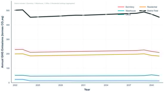
Figure 12.
Annual GHG emissions for each building and the district total. Trends reflect early grid decarbonization, gradual load increases from system aging, and a temporary peak during equipment replacement.
The Massagno district case study illustrates how the holistic LCA framework can be applied under realistic data constraints. In this context, monthly electricity data for the office building are processed through the temporal disaggregation algorithm, while annual consumption values for the remaining buildings are represented through physics-based simulation, including simulated thermal loads where fuel metering is unavailable. This mixed-data treatment strategy reflects typical deployment conditions in which monitoring infrastructure varies across buildings, and it shows how the framework can produce district-level environmental assessments despite heterogeneous data availability.
The application also highlights inherent limitations when measured consumption data do not exist. Unlike scenarios with hourly metering where temporal patterns can be validated against measured profiles, the Massagno assessment relies on simulation-generated consumption patterns throughout most of the building sector. Physics-based simulation produces hourly profiles with characteristic load patterns but reduced stochastic variation compared to measured operation. However, the dormitory’s dimensional mismatch between photovoltaic capacity and consumption magnitude eliminates uncertainty in self-consumption calculation, and the generation capacity remains sufficiently below operational loads, meaning that complete self-consumption occurs regardless of minor temporal pattern variations in simulated profiles.
5. Conclusions
This study developed and applied a holistic LCA and LCC framework that integrates three complementary components: a machine learning-based temporal disaggregation algorithm, the physics-based INTEMA simulation environment, and the VERIFY sustainability assessment tool. The framework was designed to overcome the limitations of conventional LCA practice, where aggregated or incomplete data obscure the temporal dynamics that critically influence both environmental and economic indicators. By independently reconstructing hourly electricity consumption profiles for office buildings through the data-driven disaggregation algorithm and generating thermal and other energy profiles for every building through physics-based simulation, the framework enables time-resolved LCA/LCC evaluation under conditions of heterogeneous or limited monitoring data.
The reconstructed hourly profiles produced lifecycle emission and cost estimates within 0.5% of the high-resolution reference, whereas the conventional monthly aggregation approach overestimated greenhouse gas emissions by 44.1% and altered economic indicators by 2.9%. We emphasize that this 0.5% deviation applies only to the Cardiff validation case, where measured hourly data were available, and should not be interpreted as evidence that the model’s predictive accuracy transfers to other climates, building types, or the Massagno district. This result reflects the performance of the disaggregation algorithm for UK office buildings, which is the typology used for model training and validation.
The hybrid framework was then applied at district scale through a Swiss case study, using ML-based disaggregation for the office building and physics-based simulation for the remaining buildings, with VERIFY integrating the resulting profiles for district-level LCA/LCC assessment. Over a 20-year horizon, the framework delivered a unified environmental assessment for approximately 11,600 m2 of conditioned area and an annual electricity demand of 3.9 GWh. Total district emissions reached about 9400 t CO2-eq and primary energy demand reached roughly 226 GWh, corresponding to an average carbon intensity of 41 kg CO2-eq m−2 yr−1.
Overall, this study establishes a coherent methodology for applying LCA consistently from individual buildings to districts under realistic data constraints. The hybrid workflow illustrates how ML-based disaggregation and physics-based simulation can be used in parallel within a unified LCA/LCC framework to support time-resolved environmental assessment. Future work should enhance the framework’s economic analysis, incorporate scenario-based representations of evolving grid decarbonization pathways, and extend the disaggregation model to additional building typologies and climates through training on more diverse datasets. As more monitored datasets become available, the framework should also be expanded to include error estimates derived from real measured hourly data across different building types and regions. Finally, integrating the workflow into digital-twin platforms could support real-time environmental and economic insights at larger scales.
Author Contributions
Conceptualization, G.I., R.R., P.I., S.P., N.N. and E.K.; methodology, G.I. and R.R.; software, G.I., R.R., P.I. and S.P.; validation, G.I. and R.R.; investigation, G.I.; writing—original draft preparation, G.I., R.R., P.I., S.P., N.N. and E.K.; writing—review and editing, G.I., R.R., P.I., S.P., N.N. and E.K.; visualization, G.I.; supervision, N.N. and E.K.; funding acquisition, N.N. All authors have read and agreed to the published version of the manuscript.
Funding
This work has been carried out in the framework of the European Union’s Horizon Europe research and innovation program under grant agreement No. 101069694 (DATA CELLAR project).
Data Availability Statement
The raw data supporting the conclusions of this article will be made available by the authors on request.
Acknowledgments
The authors gratefully acknowledge the contributions of Azienda Elettrica di Massagno (AEM) to the provision of specifications and data for the grid under study.
Conflicts of Interest
The authors declare no conflicts of interest.
Abbreviations
The following abbreviations are used in this manuscript:
| ASHRAE | American Society of Heating, Refrigerating and Air-Conditioning Engineers |
| BEM | Building Energy Modeling |
| COP | Coefficient of Performance |
| DTW | Dynamic Time Warping |
| DUoS | Distribution Use of System |
| ELEXON | Central Data Service Provider for the UK Electricity Market |
| ENTSO-E | European Network of Transmission System Operators for Electricity |
| EPBD | Energy Performance of Buildings Directive |
| GHG | Greenhouse Gas |
| IQR | Interquartile Range |
| LCA | Lifecycle Assessment |
| LCC | Lifecycle Costing |
| ML | Machine Learning |
| nZEB | Nearly Zero-Energy Building |
| PV | Photovoltaic |
| SLP | Standard Load Profile |
| ToU | Time-of-Use |
| VAT | Value-Added Tax |
References
- Østergaard, N.; Thorsted, L.; Miraglia, S.; Birkved, M.; Rasmussen, F.N.; Birgisdóttir, H.; Kalbar, P.; Georgiadis, S. Data Driven Quantification of the Temporal Scope of Building LCAs. Procedia CIRP 2018, 69, 224–229. [Google Scholar] [CrossRef]
- Lueddeckens, S.; Saling, P.; Guenther, E. Temporal Issues in Life Cycle Assessment—A Systematic Review. Int. J. Life Cycle Assess. 2020, 25, 1385–1401. [Google Scholar] [CrossRef]
- Frapin, M.; Roux, C.; Assoumou, E.; Peuportier, B. Modelling Long-Term and Short-Term Temporal Variation and Uncertainty of Electricity Production in the Life Cycle Assessment of Buildings. Appl. Energy 2022, 307, 118141. [Google Scholar] [CrossRef]
- Dong, J.; Schwartz, Y.; Mavrogianni, A.; Korolija, I.; Mumovic, D. A Review of Approaches and Applications in Building Stock Energy and Indoor Environment Modelling. Build. Serv. Eng. Res. Technol. 2023, 44, 333–354. [Google Scholar] [CrossRef]
- Mirabella, N.; Allacker, K.; Sala, S. Current Trends and Limitations of Life Cycle Assessment Applied to the Urban Scale: Critical Analysis and Review of Selected Literature. Int. J. Life Cycle Assess. 2019, 24, 1174–1193. [Google Scholar] [CrossRef]
- Barbero, I.; Rezgui, Y.; Beach, T.; Petri, I. Social Life Cycle Assessment in the Construction Sector: Current Work and Directions for Future Research. Int. J. Life Cycle Assess. 2024, 29, 1827–1845. [Google Scholar] [CrossRef]
- Stephan, A.; Crawford, R.H.; Bunster, V.; Warren-Myers, G.; Moosavi, S. Towards a Multiscale Framework for Modeling and Improving the Life Cycle Environmental Performance of Built Stocks. J. Ind. Ecol. 2022, 26, 1195–1217. [Google Scholar] [CrossRef]
- Walzberg, J.; Lonca, G.; Hanes, R.J.; Eberle, A.L.; Carpenter, A.; Heath, G.A. Do We Need a New Sustainability Assessment Method for the Circular Economy? A Critical Literature Review. Front. Sustain. 2021, 1, 620047. [Google Scholar] [CrossRef]
- Raventós, O.; Dengiz, T.; Medjroubi, W.; Unaichi, C.; Bruckmeier, A.; Finck, R. Comparison of Different Methods of Spatial Disaggregation of Electricity Generation and Consumption Time Series. Renew. Sustain. Energy Rev. 2022, 163, 112186. [Google Scholar] [CrossRef]
- Mihalakakou, G.; Giannadakis, A.; Malefaki, S.; Souliotis, M.; Georgiou, P.; Romaios, A.; Antzoulatou, A.; Nikolakopoulos, P.; Paravantis, J.A. Coupling Simulation-Based and Machine Learning Methodologies for Energy Optimization and Environmental Impact Mitigation in Buildings. J. Build. Eng. 2025, 112, 113809. [Google Scholar] [CrossRef]
- Lamagna, M.; Nastasi, B.; Groppi, D.; Nezhad, M.M.; Garcia, D.A. Hourly Energy Profile Determination Technique from Monthly Energy Bills. Build. Simul. 2020, 13, 1235–1248. [Google Scholar] [CrossRef]
- Smith, A.; Fumo, N.; Luck, R.; Mago, P.J. Robustness of a Methodology for Estimating Hourly Energy Consumption of Buildings Using Monthly Utility Bills. Energy Build. 2011, 43, 779–786. [Google Scholar] [CrossRef]
- Li, H.; Dai, Y.; Liu, X.; Zhang, T.; Zhang, J.; Liu, X. Feature Extraction and an Interpretable Hierarchical Model for Annual Hourly Electricity Consumption Profile of Commercial Buildings in China. Energy Convers. Manag. 2023, 291, 117244. [Google Scholar] [CrossRef]
- Marrasso, E.; Roselli, C.; Pallotta, G.; Capozzoli, A.; Buscemi, G.; Piscitelli, M.S. Novel Load-Breakdown Methodology for a University Office Building. Energy Build. 2026, 351, 116746. [Google Scholar] [CrossRef]
- Iliadis, P.; Bellos, E.; Rotas, R.; Kitsopoulou, A.; Ziozas, N.; Nikolopoulos, N.; Kosmatopoulos, E. Comprehensive Framework for Dynamic Energy Assessment of Building Systems Using IFC Graphs and Modelica. J. Build. Perform. Simul. 2025, 18, 478–499. [Google Scholar] [CrossRef]
- Kitsopoulou, A.; Pallantzas, D.; Bellos, E.; Tzivanidis, C. Mapping the Potential of Zero-Energy Building in Greece Using Roof Photovoltaics. Designs 2024, 8, 68. [Google Scholar] [CrossRef]
- Bellos, E.; Iliadis, P.; Papalexis, C.; Rotas, R.; Nikolopoulos, N.; Kosmatopoulos, E.; Halmdienst, C. Dynamic Investigation of Centralized and Decentralized Storage Systems for a District Heating Network. J. Energy Storage 2022, 56, 106072. [Google Scholar] [CrossRef]
- Skopetou, N.; Zestanakis, P.A.; Rotas, R.; Iliadis, P.; Papadopoulos, C.; Nikolopoulos, N.; Sfakianakis, A.; Koroneos, C. Energy Analysis and Environmental Impact Assessment for Self-Sufficient Non-Interconnected Islands: The Case of Nisyros Island. J. Clean. Prod. 2024, 447, 141647. [Google Scholar] [CrossRef]
- Angelakoglou, K.; Lampropoulos, I.; Chatzigeorgiou, E.; Giourka, P.; Martinopoulos, G.; Skembris, A.-S.; Seitaridis, A.; Kousovista, G.; Nikolopoulos, N. Advancing Energy-Efficient Renovation Through Dynamic Life Cycle Assessment and Costing: Insights and Experiences from VERIFY Tool Deployment. Energies 2025, 18, 3736. [Google Scholar] [CrossRef]
- Miller, C.; Kathirgamanathan, A.; Picchetti, B.; Arjunan, P.; Park, J.Y.; Nagy, Z.; Raftery, P.; Hobson, B.W.; Shi, Z.; Meggers, F. The Building Data Genome Project 2, Energy Meter Data from the ASHRAE Great Energy Predictor III Competition. Sci. Data 2020, 7, 368. [Google Scholar] [CrossRef]
- Dodd, N.; Donatello, S.; Cordella, M. Level(s) Indicator 1.2: Life Cycle Global Warming Potential (GWP); European Commission: Brussels, Belgium, 2020. [Google Scholar]
- Dodd, N.; Donatello, S.; Cordella, M. Level(s) Indicator 6.1: Life Cycle Costs; European Commission: Brussels, Belgium, 2021. [Google Scholar]
- BS 6400-2:2006; Specification for Installation, Exchange, Relocation and Removal of Gas Meters with a Maximum Capacity Not Exceeding 6 M3/h Medium Pressure (2nd Family Gases). Withdrawn. BSI: London, UK, 2006; ISBN 978-0-580-48993-8.
- BS EN 15804:2012+A1:2013; Sustainability of Construction Works. Environmental Product Declarations. Core Rules for the Product Category of Construction Products. BSI Knowledge: London, UK, 2012. Available online: https://knowledge.bsigroup.com/products/sustainability-of-construction-works-environmental-product-declarations-core-rules-for-the-product-category-of-construction-products (accessed on 1 November 2025).
- ISO 15686-5:2017; Buildings and Constructed Assets—Service Life Planning. Part 5: Life-Cycle Costing. ISO: Geneva, Switzerland, 2017. Available online: https://www.iso.org/standard/61148.html (accessed on 1 November 2025).
- Gas and Electricity Prices in the Non-Domestic Sector. Available online: https://www.gov.uk/government/statistical-data-sets/gas-and-electricity-prices-in-the-non-domestic-sector (accessed on 1 November 2025).
- DUoS Charging for LV and HV Metered Connections. Available online: https://commercial.nationalgrid.co.uk/downloads-view-reciteme/635903 (accessed on 1 November 2025).
- Electricity Maps. The World’s Most Comprehensive Electricity Data Platform. Available online: https://www.electricitymaps.com/ (accessed on 1 November 2025).
- Greenhouse Gas Reporting: Conversion Factors. 2024. Available online: https://www.gov.uk/government/publications/greenhouse-gas-reporting-conversion-factors-2024 (accessed on 1 November 2025).
- The Future Homes and Buildings Standards: 2023 Consultation. Available online: https://www.gov.uk/government/consultations/the-future-homes-and-buildings-standards-2023-consultation/the-future-homes-and-buildings-standards-2023-consultation (accessed on 1 November 2025).
- Fuel Factors Within the Home Energy Model: FHS Assessment. Available online: https://www.gov.uk/government/publications/home-energy-model-future-homes-standard-assessment-technical-documentation (accessed on 1 November 2025).
- Kousovista, G.; Iakovides, G.; Petridis, S.; Chairopoulos, N.-C.; Skembris, A.; Fotopoulou, M.; Antipa, D.; Nikolopoulos, N.; Rakopoulos, D. Comparative Lifecycle Assessment of Renewable Energy Investments in Public Buildings: A Case Study of an Austrian Kindergarten Under Atypical Operational Conditions. Appl. Sci. 2025, 15, 2330. [Google Scholar] [CrossRef]


Disclaimer/Publisher’s Note: The statements, opinions and data contained in all publications are solely those of the individual author(s) and contributor(s) and not of MDPI and/or the editor(s). MDPI and/or the editor(s) disclaim responsibility for any injury to people or property resulting from any ideas, methods, instructions or products referred to in the content. |
© 2025 by the authors. Licensee MDPI, Basel, Switzerland. This article is an open access article distributed under the terms and conditions of the Creative Commons Attribution (CC BY) license.