Abstract
Electrical strain gauges are essential for monitoring wind turbine tower loads and fatigue, but accurate load measurements from these sensors require calibration over time to correct the zero-drift found in long-term measured signals. Calibration is often performed using nacelle rotation events for cable untwisting, where the tower mechanical load is known; however, non-uniform solar heating during these events can introduce thermal stresses that are misinterpreted as drift, causing systematic errors. This study evaluates six preprocessing methods for correcting zero-drift and thermal stresses in strain gauges, using measurements from two tower cross-sections—one with temperature sensors and one without. Performance is quantified using the scatter of the 10 min mean bending moments in the fore–aft and side-to-side directions and the cumulative fatigue damage over the monitoring periods. Results show that modelling the thermal stresses using a linear regression model with temperature measurements as inputs yields the most physically consistent load curves. If temperature measurements are unavailable, the effects of thermal stresses can be partly mitigated by restricting calibration to nighttime events or using solar-position variables in a regression model (instead of temperatures). As expected, the choice of preprocessing method significantly impacts load curves, but its influence on fatigue damage estimates is limited.
1. Introduction
The transition to renewable energy is essential to mitigate the negative environmental and economic impacts of fossil fuel use, a process in which wind energy plays a central role. As of 2024, Europe had of installed wind capacity, with wind making up 19% of the consumed electricity in the European Union [1]. Many wind turbines are now approaching or have exceeded their original design life of around 20 years, prompting operators to consider life extension strategies. This trend has driven increasing research interest in the structural health monitoring (SHM) of wind turbines as a means to assess both the technical feasibility and the economic viability of extending service life [2].
Strain gauges are a common component of SHM systems for both onshore and offshore wind turbines [3,4,5], supporting applications ranging from modal identification and tracking [6] to estimating structural responses at unmeasured locations [7] and tuning numerical models [8]. All such applications rely on the accurate calculation of structural loads from the strain gauge measurements. Furthermore, since fatigue is a dominant design driver in wind turbine towers [9], estimating fatigue damage has become one of the most common uses of SHM systems with strain gauges [10,11].
Transforming strain measurements into load estimates and fatigue predictions requires careful preprocessing. Electrical strain gauges are prone to slow zero-drift, which becomes significant in long-term monitoring. In wind turbines, this drift is often estimated using cable untwisting events, during which the nacelle’s rotation imposes a known load that enables calibration. In general, these events do not occur in isothermal conditions, which may cause thermal stresses to bias zero-drift estimation, leading to systematic errors in load and fatigue calculations [12].
This work compares six approaches for deriving a correction function that converts the strain measurements recorded during cable untwisting events into mechanical stress by removing zero-drift and thermal stress. Their performance is assessed on long-term data from two instrumented cross-sections in a utility-scale wind turbine by comparing the scatter in bending moment–wind speed curves and the fatigue damage across the instrumented cross-sections. It is shown that the choice of preprocessing method has a significant impact on load estimation. On the other hand, as expected, fatigue damage estimates at the instrumented cross-sections are shown to be only marginally affected by the choice of method.
The results offer practical guidance for selecting preprocessing strategies for strain gauge measurements in wind turbine towers, taking into account the available instrumentation, the occurrence of cable untwisting events, and the intended application. When precise load estimates are required, modelling thermal stresses from local temperature measurements is recommended. If temperature data are not available, calibration restricted to nocturnal untwisting events (when conditions tend to be isothermal) can partially mitigate thermal effects, but only if a sufficient number of nighttime events exist. As an alternative, regression models based on solar-position proxies can improve load estimates without extra sensors, although with lower quality than using direct temperature measurements. For fatigue assessment, however, the choice of preprocessing method has a negligible impact, and simpler correction schemes that do not attempt to remove thermal stresses may be adequate.
2. Background
2.1. Structural Health Monitoring of Wind Turbine Towers
SHM systems are increasingly used in wind turbine towers. Depending on the monitoring objective, SHM systems may target different response quantities, most commonly vibrations or strains, with the latter being especially relevant to quantify structural loads or fatigue damage. Electrical strain gauges are very common due to their low cost and compatibility with long-term continuous measurements. Fiber-optic sensing technologies, such as Fiber Bragg Grating (FBG) strain gauges, provide a high-accuracy alternative, with multiplexing capability and immunity to electromagnetic interference, albeit with a higher cost [13]. Some disadvantages of strain gauge measurements include their sensitivity to temperature, the need for calibration and maintenance for long-term deployments, and their point-wise nature, which limits spatial resolution.
Non-contact measurement techniques, including Laser Doppler Vibrometry (LDV) [14] and Digital Image Correlation (DIC) [15], may circumvent some limitations of more traditional strain gauges. These methods provide full-field accurate and robust measurements of structural responses without physical contact with the structure. Nevertheless, their application to operational wind turbines is constrained by practical factors such as line-of-sight requirements, high deployment costs, and limited suitability for continuous long-term monitoring. As a result, strain gauges remain the predominant sensor for long-term load and fatigue assessment, and are the focus of the present work. A more detailed comparison of different sensing techniques can be found in [16].
2.2. Load Calculation from Stress Measurements
Tower bending moments are among the most important indicators for structural characterisation of wind turbines and one of the primary quantities of interest in this study. Under plane-stress conditions, the circumferential distribution of the stress caused by bending is given by
where W is the elastic section modulus, is the circumferential angle, and and are the bending moments about the x and y axes, respectively (see Figure 1). Following previous studies [10], the stress due to axial loads is not taken into account, as it is assumed constant and is a variation about this mean stress.
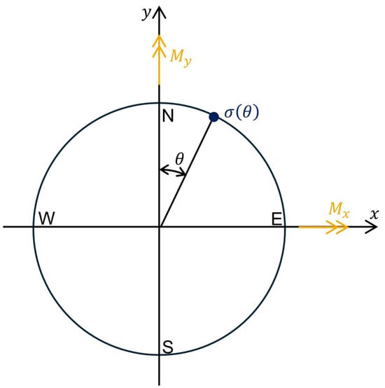
Figure 1.
Tower section coordinate system.
The bending moments are calculated from stress measurements. For a set of N measurements at angles around a section, Equation (1) yields the linear system (2), which is solved exactly for and when and estimated by least-squares when .
The turbine yaw angle defines the orientation of the rotor and nacelle relative to the x-y reference frame. The yaw angle varies with time to align the rotor with the wind direction, leading to the definition of the time-varying fore–aft (FA) and side-to-side (SS) directions, which are aligned with and perpendicular to the rotor plane, respectively, as shown in Figure 2.
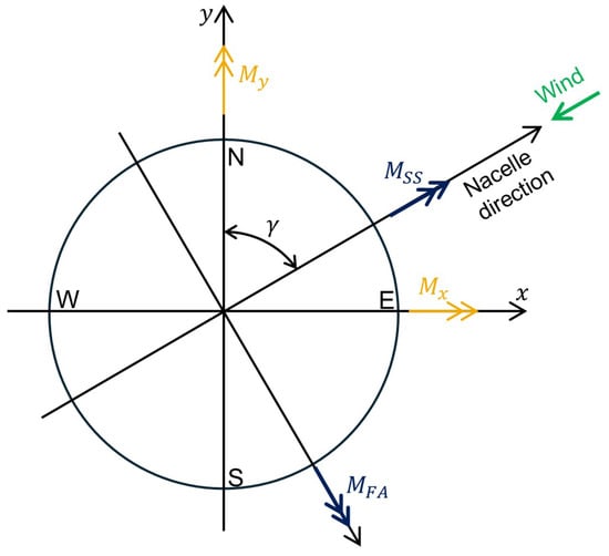
Figure 2.
Rotation to FA and SS.
Therefore, an accurate calculation of fore–aft and side-to-side bending moments requires precise knowledge of the bending-induced stress at the sensor locations, . However, in practice the measurements include additional components due to temperature effects (both physical and sensor-related) and zero-drift, as seen in the following sections.
2.3. Thermoelastic Strains and Stresses in Circular Sections
Temperature variations around the section can alter the local strain and stress fields. As illustrated in Figure 3, the circumferential temperature distribution can be decomposed as a first-harmonic part (corresponding to a uniform temperature change and a linear temperature gradient around the section with amplitude and phase ), plus the remaining higher-order part :
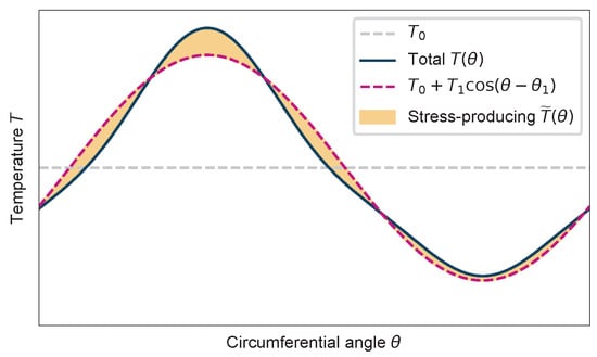
Figure 3.
Components of circumferential temperature distribution around a circular section.
In a circular section in an isostatic structure, the first-harmonic terms induce free thermal strains without generating internal stresses. In contrast, the higher-order part produces a self-equilibrated thermal strain field and the associated stress field .
The corresponding total circumferential strain is therefore given by Equation (4), where is the thermal expansion coefficient of the tower material [17].
Accordingly, the total stress is given by
Therefore, the actual stress is not always equal to the bending stress in Equation (1), since thermal stresses may be superimposed on it. This is especially relevant for wind turbine towers, where the temperature distribution can be expected to be determined mostly by solar heating, which rarely produces a first-harmonic distribution. An accurate calculation of bending moments requires removing these thermal stresses from the measurements. In previous works [10,11], thermal stresses have been mitigated by removing the means between diametrically opposed sensors, thus enforcing the symmetry that is characteristic of Equation (1). However, this approach may not always remove all thermal stresses, depending on the distribution of .
2.4. Electrical Strain Gauges
Electrical strain gauges are often employed to obtain the stress values at specific locations on wind turbine towers. These sensors measure strain by detecting small changes in the electrical resistance R of a metallic foil when deformed. Since these resistance changes are typically very small, strain gauges are commonly used in a Wheatstone bridge circuit, which arranges four resistors in a way that amplifies the measured resistance variation. When all four resistors in the bridge have equal resistance R, the output voltage is related to the input voltage through Equation (6), where is the gauge factor (given by the manufacturer and usually close to 2) and are the strains at the locations of the four resistors within the bridge.
Wheatstone bridges can be deployed in configurations where one, two, or four of the resistors are strain gauges, which are, respectively, known as quarter-bridge, half-bridge, or full-bridge. The remaining resistors can be dummy gauges (not subject to mechanical strain but affected by temperature in the same way as the active gauges) or fixed resistors. Raw strain measurements can be obtained by applying Equation (6), taking into account the bridge configuration.
Measurement using electrical strain gauges introduces some additional components to the recorded signal, which must be accounted for. These components are related to temperature variations and the long-term drift of the signal’s zero value and are described in the following sections.
2.4.1. Effect of Temperature in Strain Gauges
Several temperature-dependent effects can influence the bridge output, depending on the configuration of the strain gauge bridge [18]:
- Thermal expansion: If the strain gauge’s thermal expansion coefficient differs from that of the structure , a thermal mismatch strain appears in the measurement. This effect can be corrected if both coefficients are known; however, it is ideally minimised by using self-compensated strain gauges, designed so that matches the of the structure.
- Apparent strain: Even in self-compensated gauges, a residual thermal component remains, known as the apparent strain . Its dependence on temperature is typically provided by the manufacturer.
- Cable resistance effects: Temperature-induced changes in cable resistance can also influence the measured voltage. These effects are compensated by employing appropriate multi-wire configurations (e.g., 3- or 4-wire techniques), which ensure that resistance variations cancel within the Wheatstone bridge.
- Other effects: Other temperature-related effects include the temperature dependence of the gauge factor and the self-heating of the gauge due to the excitation voltage. However, these effects are generally small and are neglected in this study.
Temperature compensation and stress calculation is subsequently shown only for the quarter-bridge and full-bridge configurations (the latter with two dummy gauges), as they are present in the experimental setup (see Section 3.1). More details on strain gauge bridges can be found in [19].
- Quarter-bridge: only one resistor is an active gauge, while the others have a fixed resistance. Thus, the raw strain obtained by applying Equation (6) isA stress measurement can be obtained from this by compensating for thermal expansion and apparent stress and multiplying by the Young’s modulus E of the tower material:
- Full-bridge with two dummy gauges: two gauges are active, while the other two are dummy gauges, which are not subject to mechanical strain but are affected by temperature in the same way as the active gauges. This configuration inherently compensates for thermal expansion and apparent strain effects, simplifying the calculation:
2.4.2. Zero-Drift in Strain Gauges
Zero-drift is the phenomenon where the output signal from a strain gauge shifts over time, even when the actual mechanical strain on the structure remains constant. This can occur due to factors such as changes in environmental conditions and long-term creep in the gauge or adhesive [18]. In practice, these shifts manifest as a slowly varying offset in the measured stress signal, which can lead to errors in the calculated structural loads if left uncorrected. Thus, the measured stress in sensor i has a time-dependent zero-drift component , in addition to the mechanical stress and thermal stress :
Previous studies have reported varying strain gauge drift behaviour in long-term wind turbine monitoring campaigns, with the reported zero-drift behaviour varying across studies. For example, one work found that the drift rate was on the order of (or ) per year, indicating a significant variation over time [11]. Another observed that drift can vary more rapidly in certain periods while remaining almost constant in others [10]. A third study reported that tower-mounted strain gauges exhibited no drift, with the phenomenon being observed only on blade sensors [20]. In summary, strain gauge zero-drift is difficult to model a priori and must be measured.
2.5. Strain Gauge Calibration Using Cable Untwisting Events
According to the IEC standard [21], zero-drift can be corrected using measurements during cable untwisting events. These events consist of a controlled 360° rotation of the yaw angle (defined in Figure 2), carried out to relieve accumulated torsion in the tower’s internal cables due to repeated yawing during normal operation. They occur at low wind speeds, meaning that the tower bending stress is primarily due to the weight of the rotor and nacelle assembly, which has an overhang relative to the tower axis. Therefore, cable untwisting events provide a consistent and known mechanical loading, contrasting with the highly variable and unknown wind-induced loads during normal operation, making them essential for strain gauge calibration.
Figure 4 depicts the yaw angle and the measured stress at one sensor during an example event. As shown on the left side of the figure, the yaw angle varies at an approximately constant rate. Consequently, the strain gauge records an approximately sinusoidal stress response, as illustrated on the figure’s right side.
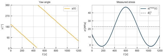
Figure 4.
Yaw angle and a tower stress measurement during a cable untwisting event.
The measured stress in sensor i can be modelled as
where A is the amplitude, is the yaw rotational speed, is a phase shift, and is the offset in sensor i during event n (also shown in Figure 4).
A comparison between Equations (10) and (11) shows that, if adequately models , then the offset is equal to the sum of the thermal stress and zero-drift components during event n. If thermal stresses are negligible during the event, then can reliably be used as an estimate of the zero-drift component at that time. If, however, thermal stresses are significant during the event—such as when there is significant solar heating on only part of the section while the other part remains shaded—the offset will include both zero-drift and thermal stress contributions, and using it as an estimate of zero-drift will introduce systematic errors in the load calculation.
2.6. Fatigue Estimation
The standard fatigue estimation approach [21,22] consists of processing stress time series using the rainflow counting algorithm [23], which identifies and quantifies the individual load cycles present in the signal. The fatigue resistance of a material is characterised by S-N curves, which define the number of cycles to failure N for a given stress amplitude S. Fatigue damage is then estimated by summing the contributions of all cycles using the Palmgren–Miner rule:
Here, is the number of cycles with amplitude within a stress range and is the corresponding number of cycles to failure, as derived from the S-N curve. The resulting damage indicator D, which aggregates the cumulative damage from M stress bins, ranges from 0 (no damage) to 1 (expected failure). In the structural analysis of wind turbines, fatigue damage is often calculated over 10-min intervals. This convention aligns with the typical resolution of turbine operational and environmental data recorded by supervisory control and data acquisition (SCADA) systems.
3. Experimental Data
3.1. Sensor Setup
This study investigates the structural response of the tower of a multi-megawatt wind turbine with a rotor diameter of 80 and hub height of 67 located in Portugal. The steel tubular tower has circular hollow cross-sections varying in diameter from at the base to at the top. SCADA data from the turbine was available, providing 10 min means of the main operational and environmental variables. Strain gauge measurements were sampled at 5 from two independent sensing systems, installed at two different locations along the tower and during different time periods. The positions of the instrumented cross-sections, along with the corresponding sensor layouts and the turbine’s wind rose, are shown in Figure 5. All sensors were installed vertically on the inner surface of the tower, at four different positions in each section in order to capture the circumferential stress distribution.
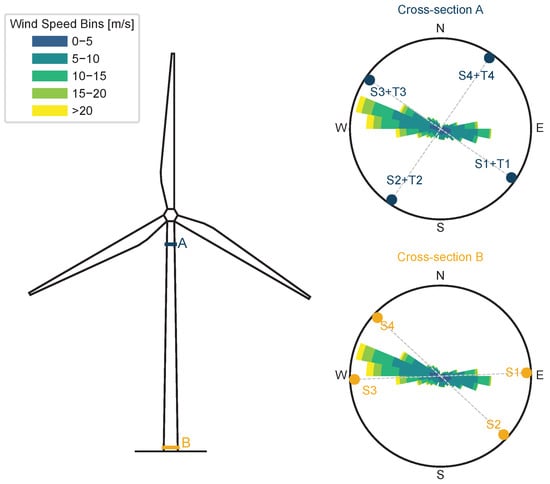
Figure 5.
Experimental setup and wind roses.
Cross-section A, located near the upper part of the tower, consists of four sensing units manufactured by Phoenix Contact (Blomberg, Germany), such as the one shown in Figure 6a. Each sensing unit consists of a quarter-bridge resistive self-compensated strain gauge and a co-located temperature sensor, a configuration which reflects a prioritization of reduced installation complexity costs. The temperature measurements are used to correct for the sensor’s sensitivity to temperature using Equation (8). More importantly, the temperature measurements also allow for a more informed correction of thermal stresses , which is the primary focus of this study. The measurements in this cross-section were collected between August 2024 and March 2025.
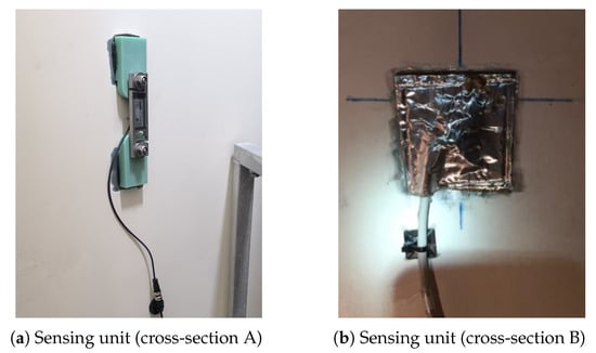
Figure 6.
Photographs exemplifying the installed sensing units in each cross-section.
Cross-section B, situated near the tower base, is instrumented with four sensing units, as shown in Figure 6b. The sensing units are full-bridge resistive self-compensated strain gauges manufactured by Hottinger Brüel & Kjær (HBK, Darmstadt, Germany), with two dummy gauges and two active gauges. No temperature measurements were available in this section. This setup provides increased sensitivity and an automatic compensation of apparent strain and thermal expansion coefficients mismatch, as explained in Section 2.4.1. However, the lack of insight into the circumferential temperature distribution limits the ability to correct for thermal stresses. The data analysed for cross-section B corresponds to the time period from January to December 2020.
3.2. Cable Untwisting Events
As explained in Section 2.5, strain gauge calibration typically relies on cable untwisting events. A total of 15 cable untwisting events were recorded during the monitoring period of cross-section A and 32 events in the monitoring period of cross-section B. The measurement offsets (corresponding to sensor i during event n) were extracted from each event by fitting Equation (11). The resulting offsets for all events and sensors are presented in Figure 7.
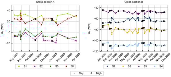
Figure 7.
Cable untwisting events offsets .
The evolution of the measured offsets over time is non-monotonic, with certain events showing sharp deviations from adjacent events. Notably, these abrupt changes occur simultaneously across several sensors. This behaviour strongly indicates that the offset variation is influenced by environmental effects. As explained in Section 2.5, untwisting events occur under very low wind speeds, so the observed variations are most plausibly attributed to thermal stresses.
In addition, Figure 7 highlights the offset values obtained with untwisting events that occurred during the night. In cross-section B, whose monitoring period has a higher number of nocturnal events, it can be seen that these events tend to follow a smoother trend, with the more abrupt deviations being found in events recorded during the day. This agrees with the hypothesis that non-uniform solar heating determines thermal stresses that affect this calibration procedure.
4. Methods for Drift and Residual Stress Correction
4.1. Overview
The present section describes the necessary preprocessing to obtain corrected mechanical stress time series from the stress signals measured from the strain gauge circuits (Section 2.4). In generic terms, this consists of subtracting a correction function from the measured signal:
According to Equation (10), the correction function must account for both zero-drift and thermal stress :
Table 1 summarises the correction methods used to define the correction function in various ways. Methods LI-N and LF-N rely on the thermal uniformity of nocturnal untwisting events and are therefore only applicable to cross-section B, as cross-section A did not record a sufficient number of nighttime events. Conversely, methods requiring temperature measurements are only applicable to cross-section A, since cross-section B lacks temperature data. A detailed description of each method is provided in Section 4.2.

Table 1.
Summary of methods to correct thermal stress and zero-drift .
4.2. Description of Correction Methods
4.2.1. LI—Enforcing Symmetry with Linearly Interpolated Zero-Drift
The first method, which follows [10], begins by forcing the mean of each pair of opposite sensors to zero. This is based on the plane stress assumption, which implies that opposite points on the section experience equal and opposite stresses:
It should be noted that the assumption that this step removes thermal stresses is only valid if the thermal stress distribution is negligible, symmetric, or first-harmonic. As explained in Section 2.3, this is often not the case due to solar heating.
Applying this step to four sensors produces two pairs of symmetrical signals. With two independent signals, the bending moments can be computed directly from Equation (2), providing an exact solution that is both computationally efficient and physically consistent. The assumption that enforcing symmetry removes implies that is exactly equal to the cable untwisting event offset during event n. Between events n and , is obtained by linearly interpolating the corresponding offsets and . Mathematically, this method can be expressed with Equation (16), where the indices i and j correspond to a pair of opposite sensors.
4.2.2. LI-N—Enforcing Symmetry with Linearly Interpolated Zero-Drift, Using Nocturnal Events Only
Method LI-N follows the same procedure as Method LI, but it only uses cable untwisting events that occurred during the night for the linear interpolation. The reasoning is that, at night, the section temperatures are generally more uniform, since there is no sunlight to cause local heating. Under these conditions, the thermal stress is expected to be minimal, making the estimation of zero-drift from the event offsets more reliable.
4.2.3. LF—Enforcing Symmetry with Linear Zero-Drift
Method LF builds directly on the previous method LI. The first step of removing the means between opposite sensors remains unchanged. However, the zero-drift is assumed to vary linearly in time:
The coefficients and are obtained via a least-squares fit to the offsets , calculated in the cable untwisting events. This provides a smoother zero-drift correction, which is expected to be less sensitive to abrupt variations in the offsets that may be caused by thermal stresses during the events. However, the assumption that drift varies linearly is not supported by a physical model and may be an oversimplification of the actual drift behaviour.
4.2.4. LF-N—Enforcing Symmetry with Linear Zero-Drift, Using Nocturnal Events Only
Method LF-N corresponds to method LF, using only the offsets from cable untwisting events which occurred at night.
4.2.5. TR—Temperature-Based Thermal Stress Regression with Linear Zero-Drift
Method TR adopts a different approach to modeling thermal stress, leveraging the availability of temperature measurements in the section. Instead of enforcing symmetry by removing the means of opposite sensors, the thermal stress is modelled as a linear function of the individual sensor temperatures relative to the mean temperature across the four sensors. This formulation reflects the assumption that thermal stresses are primarily driven by local temperature gradients. The zero-drift is assumed to vary linearly with time. In total, this approach involves six linear regression coefficients, all of which are determined using the cable untwisting event offsets .
Note that method TR implies that the bending moments and are determined from Equation (1) using a least-squares fit to 4 values of . This is a difference relative to the remaining methods, where the enforced symmetry yields only 2 independent stress time series and therefore Equation (1) is solved exactly.
4.2.6. PR—Proxy-Based Thermal Stress Regression with Linear Zero-Drift
Method PR replaces the direct use of temperature measurements with a set of proxy variables derived from the solar geometry at the turbine location. The predictors are the solar time, solar elevation, and solar azimuth, which are closely related to the temperature field in the section and do not require any additional sensors. These were calculated using the pvlib Python package, version v0.12.0 [24], knowing the wind turbine’s latitude and longitude. These predictors are expressed as sine and cosine components to capture their cyclic nature and are set to zero at night, with a smoothing function to transition gradually between daytime and nighttime.
The thermal stress at sensor i is modelled as a linear function of these proxy variables, along with a zero-drift term that varies linearly in time:
where are the weighted proxy variables. As in method TR, the regression coefficients are determined using the cable untwisting event offsets , but unlike TR, this formulation does not require direct temperature measurements, enabling application in cross-section B. Although PR is expected to be a lower-accuracy alternative to TR to be applied when temperature measurements are unavailable, it was also applied to cross-section A. This enables a direct comparison between the two regression-based approaches under identical conditions, evaluating the performance benefits of using actual temperature data.
5. Results and Discussion
5.1. Bending Moments
The correction methods described in Section 4 were applied to the 10 min means of the measured stress signals, yielding corrected mechanical stresses . These corrected signals were then used to compute the bending moments and at each instrumented section, using Equation (1), and subsequently rotated to obtain the fore–aft and side-to-side components, and , using the SCADA 10 min mean yaw time series .
This section presents a comparison of the bending moment estimates as a function of the 10 min means of wind speed V (obtained from the SCADA system) for each correction method and in each section (when applicable, as per Table 1). In addition to the visual comparison of load curves, a Load Scatter Index (LSI) is introduced as a quantitative measure of the consistency of the results: the wind speed range is divided into bins of , and the standard deviation of moment values is computed within each bin. The LSI is defined as the mean of these standard deviations across all bins. A lower value indicates a cleaner load curve and, therefore, a more effective correction. When comparing the two cross-sections, it should be noted that their different heights lead to different load ranges, with cross-section A experiencing lower bending moments, which also contributes to the observed performance differences when measured through the LSI.
5.1.1. Bending Moments in Cross-Section A
Figure 8 shows the load curves obtained by applying the linear interpolation method (LI), the linear fit method (LF), the temperature-based regression method (TR), and the proxy-based regression method (PR) in cross-section A, showcasing significant differences between methods. Since in this section the bending moments are quite small, when compared to those observed at the tower base, the achievement of accurate estimates is much more difficult.
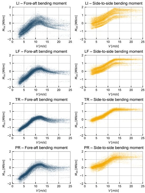
Figure 8.
Loads calculated from 10 min means of stress signals with different correction strategies in cross-section A (fore-aft and side-to-side directions).
The LI method shows the highest levels of scatter. This can be attributed to its simplistic treatment of zero-drift: the method misinterprets temperature-induced fluctuations in the offset values as zero-drift, causing unrealistic corrections in the stress signals and, consequently, in the calculated loads. Method LF, which models the zero-drift with a linear trend, reduces this effect to some extent by smoothing out the fluctuations. Nevertheless, it still does not yield a single unified trend in the load curves.
The TR method yields the least-scattered bending moment values, indicating a more effective suppression of thermal stress due to its direct, data-driven modeling approach. The PR method produces intermediate scatter, but unlike LI and LF—which tend to generate separate trend lines as a result of systematic thermal-stress misinterpretation—PR exhibits scatter around a single coherent trend, suggesting that its results are more physically consistent. This effect is particularly evident in the side-to-side bending moment.
These qualitative observations are supported by the LSI results in Figure 9. TR achieves the lowest LSI, confirming its superior reliability, while LI produces the highest scatter. Overall, these results highlight the benefit of incorporating temperature information in cross-section A to directly model and remove the thermal stress component, as in TR, which more consistently recovers the expected physical relationship between wind loading and tower bending moments.
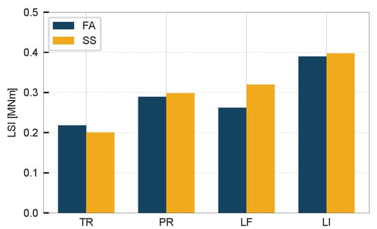
Figure 9.
Load Scatter Index in different methods in cross-section A.
5.1.2. Bending Moments in Cross-Section B
In cross-section B, the absence of temperature measurements prohibited the use of method TR. Alternative strategies to mitigate thermal stresses consisted of filtering to nighttime events and using solar proxies for regression. Accordingly, five correction methods were applied: the linear interpolation method (LI), the linear fit method (LF), their nocturnal-event-only counterparts (LI-N and LF-N), and the proxy-based regression method (PR). Figure 10 presents the bending moment curves derived from each method, while Figure 11 compares their Load Scatter Index (LSI) values.
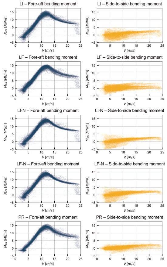
Figure 10.
Loads calculated from 10-min means of stress signals with different correction strategies in cross-section B (fore-aft and side-to-side directions).
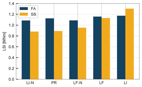
Figure 11.
Load Scatter Index for different methods in cross-section B.
As in cross-section A, the LI method produces the largest scatter, confirming that its simplistic zero-drift treatment fails to address residual thermal effects. LF offers moderate improvement by smoothing the drift via a linear trend, but the overall reduction in scatter remains limited. Filtering to nocturnal events (LI-N and LF-N) yields a further decrease in the LSI, with LI-N marginally outperforming LF-N. Upon further investigation, it was observed that deviations from the main trends in both nocturnal methods occur mainly between May and July 2020, when no nighttime events were recorded.
The PR method again yields moderate scatter centered on a single coherent trendline. It is interesting to note that its scatter increases at higher wind speeds. This is likely due to enhanced convective cooling under strong winds, which tends to homogenise the circumferential temperature field, weakening the correlation between the selected proxies and the thermal stresses. This limitation is inherent to the PR method, independently of what proxies are used, because the calibration is done using only untwisting events, which always occur at low wind speeds. Therefore, the model is not informed about the high-wind regime, where convective cooling becomes relevant.
These results confirm that nocturnal filtering can be an effective substitute when direct temperature compensation is not possible, though its effectiveness is still limited compared to TR in cross-section A. Moreover, reliance on nighttime events can reduce the available calibration dataset, potentially making the method impractical for shorter monitoring periods. In such cases, PR offers a viable alternative. Overall, the findings reinforce that while symmetry enforcement, nocturnal filtering, and solar-based proxy variables help reduce thermal effects, none match the precision of direct temperature-based correction.
5.2. Fatigue Damage
Fatigue damage was calculated at 36 equally spaced circumferential points in each instrumented section, using the corrected mechanical stress time series obtained using Equation (1) with each preprocessing method. Due to the geometrical symmetry in plane stress conditions (Equation (15)), results are presented only for the range . For each , the cumulative damage D was obtained by summing the damage from all 10-min segments in the analysis period. The damage calculation in each interval was done using the py-fatigue Python package, version v2.0.3 [25].
5.2.1. Fatigue Damage in Cross-Section A
Figure 12 shows the cumulative fatigue damage for cross-section A across all angles, for each of the four correction methods (LI, LF, TR, and PR).
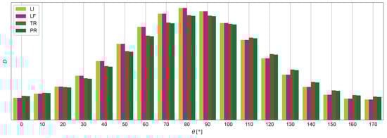
Figure 12.
Fatigue damage estimated with different correction strategies in cross-section A.
The LI and LF methods yield essentially identical results, producing nearly overlapping curves across the entire section. Similarly, the TR and PR methods show close agreement with each other. The main difference lies between these two groups: LI/LF and TR/PR produce distinct shapes for the fatigue damage distribution across the section. This divergence is attributed to the different strategies used to correct thermal stresses—LI and LF enforce symmetry between opposite sensors, while TR and PR apply regression models, which yield slightly different shapes of for each time instant.
Despite these differences, all methods identify the same angular position of maximum fatigue damage at , indicating that the choice of correction method does not affect the location of the most fatigue-critical angle. The largest percentual difference between methods at the critical is %, while the largest difference between methods across the entire section is % and occurs at . These differences between methods can be considered negligible.
5.2.2. Fatigue Damage in Cross-Section B
Figure 13 compares the five methods applied in cross-section B (LI, LF, LI-N, LF-N, and PR) and confirms that the choice of thermal stress removal approach drives the main differences in fatigue estimates. All symmetry-enforcing methods (LI, LF, LI-N, and LF-N) yield closely matching distributions, whereas PR shows the most noticeable deviations.
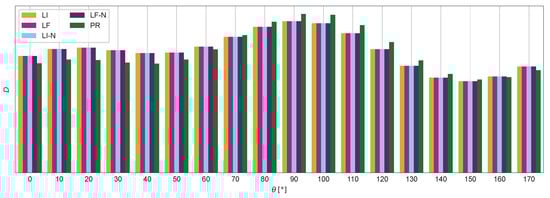
Figure 13.
Fatigue damage estimated with different correction strategies in cross-section B.
The largest discrepancies occur in angular regions without strain gauge coverage (see Figure 1 and Figure 5). In particular, the maximum deviation in D (11.3%) is observed at . As in cross-section A, these differences reflect the fact that the methods produce different instantaneous stress distributions . All methods agree on the critical angle, , where the deviation between them is only 4.9%.
As with cross-section A, the observed deviations translate into negligible lifetime differences in practical terms. This is expected, because changing the preprocessing method does not significantly alter the stress cycle amplitudes, which dominate fatigue. As a result, an extrapolation of the observed damage differences to a full turbine lifetime would not change any engineering conclusions regarding fatigue life in either section.
6. Conclusions
This study evaluated six strain gauge preprocessing methods for correcting zero-drift and thermal stresses in wind turbine tower measurements, aiming to enhance accuracy in load calculation and fatigue life estimation. Two instrumented tower cross-sections with differing sensor configurations were considered, and all methods used the measured offsets during cable untwisting events as a starting point for calibration. The methods highlight the importance of removing thermal stresses in cable untwisting events, avoiding their misinterpretation as zero-drift.
The temperature-based regression method (TR), which models thermal stresses from measured temperatures, produced the most physically consistent load curves. When temperature data were unavailable, two alternative strategies were considered: restricting calibration to nocturnal events (LI-N and LF-N) and building a regression model from solar-position-based proxy variables (PR). The nocturnal-event methods are limited by event availability, while PR shows increasing scatter at higher wind speeds. Both alternatives achieved partial thermal-stress removal, but neither matched the performance of TR.
For fatigue damage, results in both cross-sections showed that methods fell into two consistent groups, distinguished by their thermal stress removal strategies: symmetry-enforcing methods (LI, LF, LI-N, and LF-N) and regression-based methods (TR, and PR). Differences between these groups were primarily in the shape of the circumferential damage distribution . However, all methods identified the same critical angular position, with small differences in its accumulated damage estimation.
Overall, these results show that relying solely on cable untwisting events for calibration can lead to significant errors in load estimation if thermal effects are ignored. Careful selection of the preprocessing method—ideally one using temperature measurements—is essential for accurate load assessment. For fatigue estimation, the choice of method has a smaller impact but still influences the damage distribution shape in each section.
Author Contributions
Conceptualization, F.M., J.P.S., A.B. and A.G.; methodology, A.G.; software, A.G.; validation, A.B., F.M. and J.P.S.; formal analysis, A.G.; investigation, A.G.; resources, A.B.; data curation, A.G.; writing—original draft preparation, A.G.; writing—review and editing, A.G., A.B., F.M. and J.P.S.; visualization, A.G.; supervision, F.M. and J.P.S.; project administration, F.M. and J.P.S.; funding acquisition, F.M. and J.P.S. All authors have read and agreed to the published version of the manuscript.
Funding
This work was funded by the Foundation for Science and Technology (Fundação para a Ciência e Tecnologia, FCT) through the PhD grant 2022.12813.BD, Base Funding IDB/04708/2020 of CONSTRUCT—Instituto de I&D em Estruturas e Construções, and the project 2022.08120.PTDC (M4WIND, https://doi.org/10.54499/2022.08120.PTDC), funded by national funds through the FCT/MCTES (PIDDAC).
Data Availability Statement
The data presented in this study are available on request from the corresponding author and have not been published due to confidentiality agreements with the data provider.
Acknowledgments
The authors wish to thank Nadara for kindly providing the wind turbine measurement data that made this work possible.
Conflicts of Interest
Authors André Biscaya and João P. Santos were employed by the company Nadara. The remaining authors declare that the research was conducted in the absence of any commercial or financial relationships that could be construed as a potential conflict of interest.
Abbreviations
The following abbreviations are used in this manuscript:
| SHM | Structural Health Monitoring |
| SCADA | Supervisory Control and Data Acquisition |
| FA | Fore–Aft |
| SS | Side to Side |
| LI | Linear Interpolation |
| LI-N | Linear Interpolation—Nocturnal |
| LF | Linear Fit |
| LF-N | Linear Fit—Nocturnal |
| TR | Temperature-based Regression |
| PR | Proxy-based Regression |
| LSI | Load Scatter Index |
References
- Constanzo, G.; Brindley, G.; Tardieu, P. Wind Energy in Europe: 2024 Statistics and the Outlook for 2025–2030; Technical Report; WindEurope: Brussels, Belgium, 2025. [Google Scholar]
- Rubert, T.; Zorzi, G.; Fusiek, G.; Niewczas, P.; McMillan, D.; McAlorum, J.; Perry, M. Wind turbine lifetime extension decision-making based on structural health monitoring. Renew. Energy 2019, 143, 611–621. [Google Scholar] [CrossRef]
- Simoncelli, M.; Zucca, M.; Ghilardi, M. Structural health monitoring of an onshore steel wind turbine. J. Civ. Struct. Health Monit. 2024, 14, 1423–1437. [Google Scholar] [CrossRef]
- Pimenta, F.; Ribeiro, D.; Román, A.; Magalhães, F. Modal properties of floating wind turbines: Analytical study and operational modal analysis of an utility-scale wind turbine. Eng. Struct. 2024, 301, 117367. [Google Scholar] [CrossRef]
- Hines, E.M.; Baxter, C.D.P.; Ciochetto, D.; Song, M.; Sparrevik, P.; Meland, H.J.; Strout, J.M.; Bradshaw, A.; Hu, S.L.; Basurto, J.R.; et al. Structural instrumentation and monitoring of the Block Island Offshore Wind Farm. Renew. Energy 2023, 202, 1032–1045. [Google Scholar] [CrossRef]
- Pereira, S.; Pacheco, J.; Pimenta, F.; Moutinho, C.; Cunha, A.; Magalhães, F. Contributions for enhanced tracking of (onshore) wind turbines modal parameters. Eng. Struct. 2023, 274, 115120. [Google Scholar] [CrossRef]
- Iliopoulos, A.; Weijtjens, W.; Van Hemelrijck, D.; Devriendt, C. Fatigue assessment of offshore wind turbines on monopile foundations using multi-band modal expansion. Wind Energy 2017, 20, 1463–1479. [Google Scholar] [CrossRef]
- Moynihan, B.; Mehrjoo, A.; Moaveni, B.; McAdam, R.; Rüdinger, F.; Hines, E. System identification and finite element model updating of a 6 MW offshore wind turbine using vibrational response measurements. Renew. Energy 2023, 219, 119430. [Google Scholar] [CrossRef]
- Burton, T.; Jenkins, N.; Bossanyi, E.; Sharpe, D.; Graham, M. Wind Energy Handbook, 3rd ed.; John Wiley & Sons Ltd.: Hoboken, NJ, USA, 2021. [Google Scholar]
- Pacheco, J.; Pimenta, F.; Pereira, S.; Cunha, A.; Magalhães, F. Fatigue Assessment of Wind Turbine Towers: Review of Processing Strategies with Illustrative Case Study. Energies 2022, 15, 4782. [Google Scholar] [CrossRef]
- Loraux, C.; Brühwiler, E. The use of long term monitoring data for the extension of the service duration of existing wind turbine support structures. J. Phys. Conf. Ser. 2016, 753, 072023. [Google Scholar] [CrossRef]
- Bezziccheri, M.; Castellini, P.; Evangelisti, P.; Santolini, C.; Paone, N. Measurement of mechanical loads in large wind turbines: Problems on calibration of strain gage bridges and analysis of uncertainty. Wind Energy 2017, 20, 1997–2010. [Google Scholar] [CrossRef]
- Bang, H.J.; Kim, H.I.; Lee, K.S. Measurement of strain and bending deflection of a wind turbine tower using arrayed FBG sensors. Int. J. Precis. Eng. Manuf. 2012, 13, 2121–2126. [Google Scholar] [CrossRef]
- Chen, Y.; Griffith, D.T. Experimental and numerical full-field displacement and strain characterization of wind turbine blade using a 3D Scanning Laser Doppler Vibrometer. Opt. Laser Technol. 2023, 158, 108869. [Google Scholar] [CrossRef]
- Feng, W.; Yang, D.; Du, W.; Li, Q.; Feng, W.; Yang, D.; Du, W.; Li, Q. In Situ Structural Health Monitoring of Full-Scale Wind Turbine Blades in Operation Based on Stereo Digital Image Correlation. Sustainability 2023, 15, 13783. [Google Scholar] [CrossRef]
- Civera, M.; Surace, C. Non-Destructive Techniques for the Condition and Structural Health Monitoring of Wind Turbines: A Literature Review of the Last 20 Years. Sensors 2022, 22, 1627. [Google Scholar] [CrossRef] [PubMed]
- Loraux, C.T. Long-Term Monitoring of Existing Wind Turbine Towers and Fatigue Performance of UHPFRC Under Compressive Stresses. Ph.D. Thesis, EPFL, Lausanne, Switzerland, 2018. [Google Scholar] [CrossRef]
- HBK. Strain Gauges: How to Prevent Temperature Effects on Your Measurement. Available online: https://www.hbkworld.com/en/knowledge/resource-center/articles/strain-measurement-basics/strain-gauge-fundamentals/article-temperature-compensation-of-strain-gauges (accessed on 13 November 2025).
- Hoffmann, K. Applying the Wheatstone Bridge Circuit; Technical Report S1569-1.3 en; HBM: Natick, MA, USA, 1974. [Google Scholar]
- Faria, B.R.; Dimitrov, N.; Perez, V.; Kolios, A.; Abrahamsen, A.B. Virtual load sensors based on calibrated wind turbine strain sensors for damage accumulation estimation: A gap-filling technique. J. Phys. Conf. Ser. 2025, 3025, 012011. [Google Scholar] [CrossRef]
- IEC. Wind Turbines Part 13: Measurement of Mechanical Loads; IEC: Geneva, Switzerland, 2015. [Google Scholar]
- IEA. Recommended Practices for Wind Turbine Testing and Evaluation. 3. Fatigue Loads; Technical Report; International Energy Agency: Paris, France, 1990. [Google Scholar]
- Matsuichi, M.; Endo, T. Fatigue of Metals Subjected to Varying Stress. 1968. Available online: https://www.semanticscholar.org/paper/Fatigue-of-metals-subjected-to-varying-stress-Matsuichi-Endo/467c88ec1feaa61400ab05fbe8b9f69046e59260#related-papers (accessed on 13 November 2025).
- Anderson, K.S.; Hansen, C.W.; Holmgren, W.F.; Jensen, A.R.; Mikofski, M.A.; Driesse, A. pvlib python: 2023 project update. J. Open Source Softw. 2023, 8, 5994. [Google Scholar] [CrossRef]
- D’Antuono, P.; Weijtjens, W.; Devriendt, C. Py-Fatigue. 2022. Available online: https://owi-lab.github.io/py_fatigue (accessed on 13 November 2025).
Disclaimer/Publisher’s Note: The statements, opinions and data contained in all publications are solely those of the individual author(s) and contributor(s) and not of MDPI and/or the editor(s). MDPI and/or the editor(s) disclaim responsibility for any injury to people or property resulting from any ideas, methods, instructions or products referred to in the content. |
© 2025 by the authors. Licensee MDPI, Basel, Switzerland. This article is an open access article distributed under the terms and conditions of the Creative Commons Attribution (CC BY) license.