Investigation of Residential Value of Lost Load and the Importance of Electric Loads During Outages in Japan

Abstract

Reducing damage caused by power outages is important against the background of severe natural disasters. Estimating the value of lost load (VoLL) is key to making an optimal investment plan for power systems. This paper aims to estimate the recent residential VoLL in Japan by using a survey. The contingent valuation method quantifies the residential willingness to pay (WTP) and its distribution in a 2 h outage during summer. When combining actual demand data, the VoLL is estimated at 501.1 JPY/kWh for a predictable outage and 559.9 JPY/kWh for a sudden one. In addition, the random utility model reveals the effect of people’s attributes on WTP. Larger annual incomes and electricity bills significantly increase WTP. Evacuation experiences and stockpiles also affect WTP in a sudden outage. Finally, 80% of respondents answered that refrigerators, air conditioners, and water supplies are important during outages.

1. Introduction

Electricity is the basis of today’s society, supporting other infrastructures, such as transportation, communication, and water supply. Thus, power supply interruptions have a great impact on our lives. Recently, severe natural disasters have damaged power systems and caused large supply interruptions. In Texas, a severe winter storm caused the loss of 30 GW of power generation and a blackout in February 2021 [1]. This blackout affected 4.5 million households in Texas and around 10 million people [1]. In Japan, typhoon No. 15 (Faxai) caused widespread damage to transmission and distribution networks in the Kanto region [2], and it caused a lengthy blackout that affected around 1 million households. It took over 10 days to recover the electricity supply of 99% of households [2]. Along with severe climate disasters, large earthquakes have caused severe blackouts in Japan. One example is the Hokkaido Eastern Iburi Earthquake in 2018. It caused a blackout in the whole Hokkaido region and affected around 3 million people [3] in 2 days. These supply shortages emphasize the importance of a resilient power system that sustains its normal function during severe disasters.

Measures to reduce supply shortages enable society to avoid costs caused by power outages. Some of the measures require investment, such as reinforcing transmission lines and introducing emergency generators. The value of avoiding power outages using these measures should be evaluated to make optimal investment plans. In addition, this value helps to plan for optimal rolling blackouts when the power supply becomes low [4,5]. The value of lost load (VoLL) is the most popular indicator of cost [6,7,8]. It expresses the costs of power outages in terms of electricity not supplied [$\mathrm{kWh}$].

The VoLL has been estimated by power system operators [9,10,11] and researchers [12,13,14,15,16,17,18] in many countries. The VoLL differs between sectors, such as industry, service, and households. Residential VoLL expresses the discomfort caused by power outages [19]. It ranges widely because of the difference in power systems and household discomfort. Ref. [19] summarizes residential VoLL, ranging between 0–40 $\mathrm{USD}/\mathrm{kWh}$. Regarding Japan, ref. [20] estimated residential VoLL in Hokkaido, ranging between 1350–2700 $\mathrm{JPY}/\mathrm{kWh}$. A cross-regional operator estimated residential VoLL in 2013, ranging between 4300–8100 $\mathrm{JPY}/\mathrm{kWh}$ [9]. After the Great East Japan Earthquake in 2011, the power system in Japan changed, with a halt to nuclear power plant operations, the large-scale introduction of solar power, and the deregulation of power generation and retail. People’s VoLLs may differ from the values stated in previous research. However, we are not aware of any studies conducted in Japan in recent years. In addition, previous research in Japan does not show the distribution of VoLLs. Estimating their distribution helps in terms of making a better investment plan for the power system.

VoLL varies depending on a person’s attributes. Analyzing the effect of attributes helps estimate residential VoLL. Previous research analyzed the relationship between VoLL and attributes [12,14,15,21]. Attributes such as gender, age, occupation, and using electric heating are found to affect residential VoLL in the northwest of England [15]. In contrast, research in Korea [21] shows that monthly income significantly affects VoLL, but age and the number of family members do not. In Japan, we have not seen any analysis of personal attributes that affect residential VoLL.

Electricity demand includes both essential loads and unimportant loads during outages. The VoLL of each load can differ according to its importance. For example, medical apparatus have high VoLL values because they directly affect life [22]. In contrast, ceiling lights have low VoLL values because people can easily use substitutional goods like candles. Investigating the importance of residential loads helps estimate the amount of essential loads during outages. For power system operators, it results in a more precise estimation of costs according to outages in the residential sector. In addition, it helps evaluate a household’s resilience [23]. However, it is not yet enough to investigate the important loads in households.

Measures against supply shortages are important in severe natural disasters. A survey of the current VoLL can help stakeholders decide the optimal measures for power systems and consumers. This paper aims to investigate current residential VoLL values and the importance of electric loads in Japan using a survey. The main contributions of this paper are as follows:

• This paper estimates the representative value and distribution of residential VoLL by using a contingent valuation method (CVM);
• This paper uses a random utility model to analyze the significance of respondents’ attributes on VoLL;
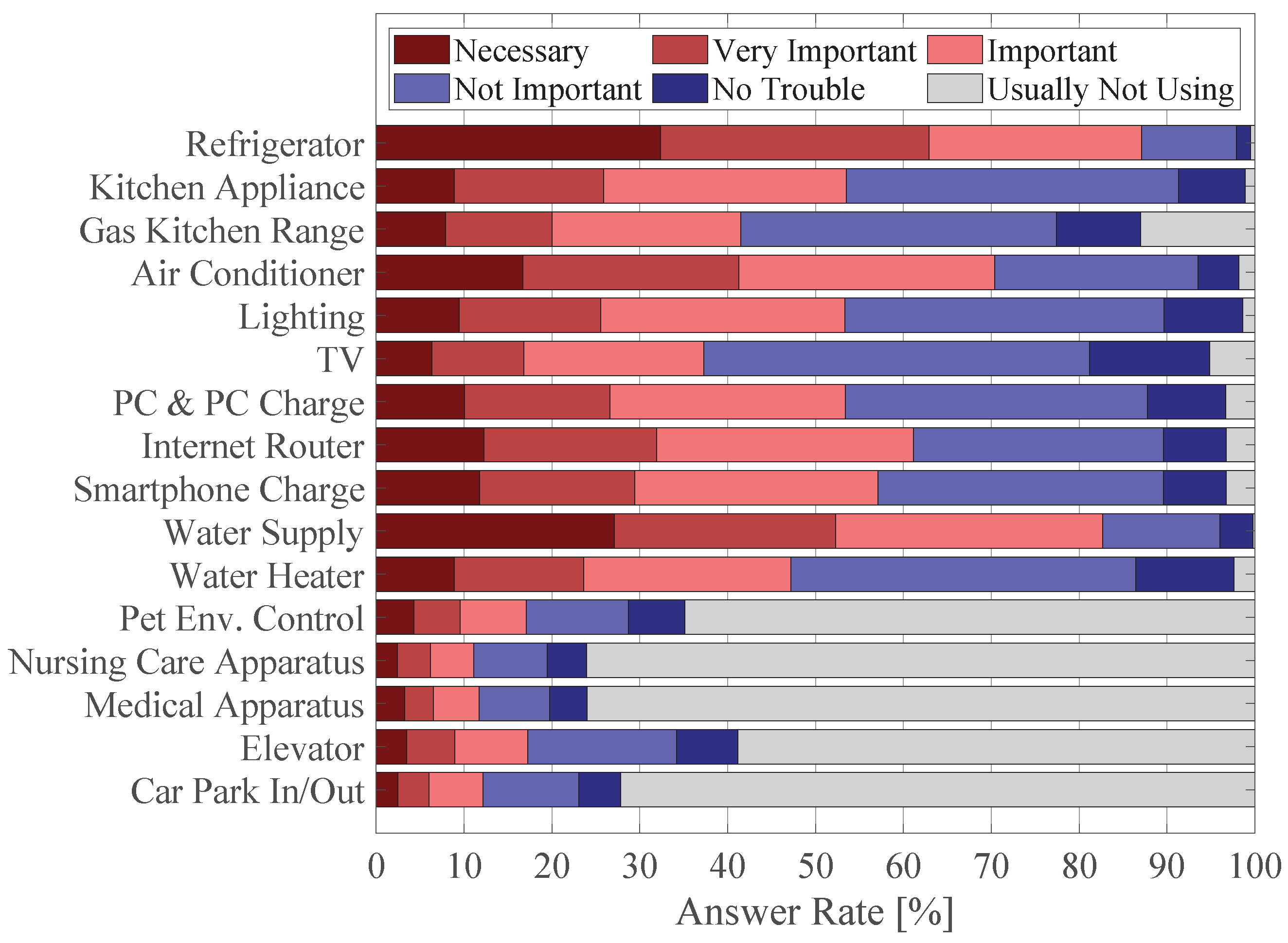
• This paper investigates the importance of each load in households by using a survey.

The remainder of this paper is organized as follows. The method to estimate the residential VoLL is described in Section 2.

The results of the survey and estimation of VoLL are expressed in Section 3. The effect of individual attributes on VoLL is analyzed in Section 4. The importance of each load is described in Section 5. Finally, the conclusion is presented in Section 6.

2. Method

2.1. Overview of Value of Lost Load Estimation

The value of lost load (VoLL) is the quantified economic loss or discomfort caused by a power outage [19]. Unlike electricity, supply interruptions are not traded in the market. Thus, there is no explicit price expressing the cost of outages. The VoLL should be estimated by calculating the damage caused by outages. There are several methods to calculate the damage:

• Stated preference method [12,13,14,16,17,18,24]. This method uses the results of surveys and interviews to determine the damage caused by outages. The survey and interview inquire into how much people are willing to pay to avoid the damage, how much they are willing to accept (at least as compensation) for outages, or which kind of outages they prefer. There are biases in terms of the stated values due to several causes, such as survey methods, questionnaire structures, and respondents’ bounded rationality [25].
• Revealed preference method [14]. This estimates the VoLL using expenditures on backup equipment, such as emergency power generators and contracts that enable supply interruption. However, households tend to use such equipment rarely. Thus, this method can overestimate the cost of outages per hour.
• Macroeconomic method [4,26,27]. This estimates losses in industrial, commercial, and residential sectors using regional statistical data. Input/output tables and annual electricity consumption are collected to estimate the economic loss caused by outages. The residential cost of outages is considered the loss of leisure time. In the estimation, residential VoLL is assumed to equal people’s work wage. This method makes it challenging to investigate the distribution of costs in terms of outages.
• Case study [28]. This method accumulates the damage caused by actual supply interruptions. It can calculate the actual damage. However, it is difficult to generalize the result because the outage is not always representative.

This paper tries to estimate the distribution of residential VoLL. The power system in Japan is very reliable, and outages rarely happen. Thus, the revealed preference method will overestimate the VoLL. The macroeconomic method makes it challenging to estimate the distribution. Hence, this paper chooses the stated preference method.

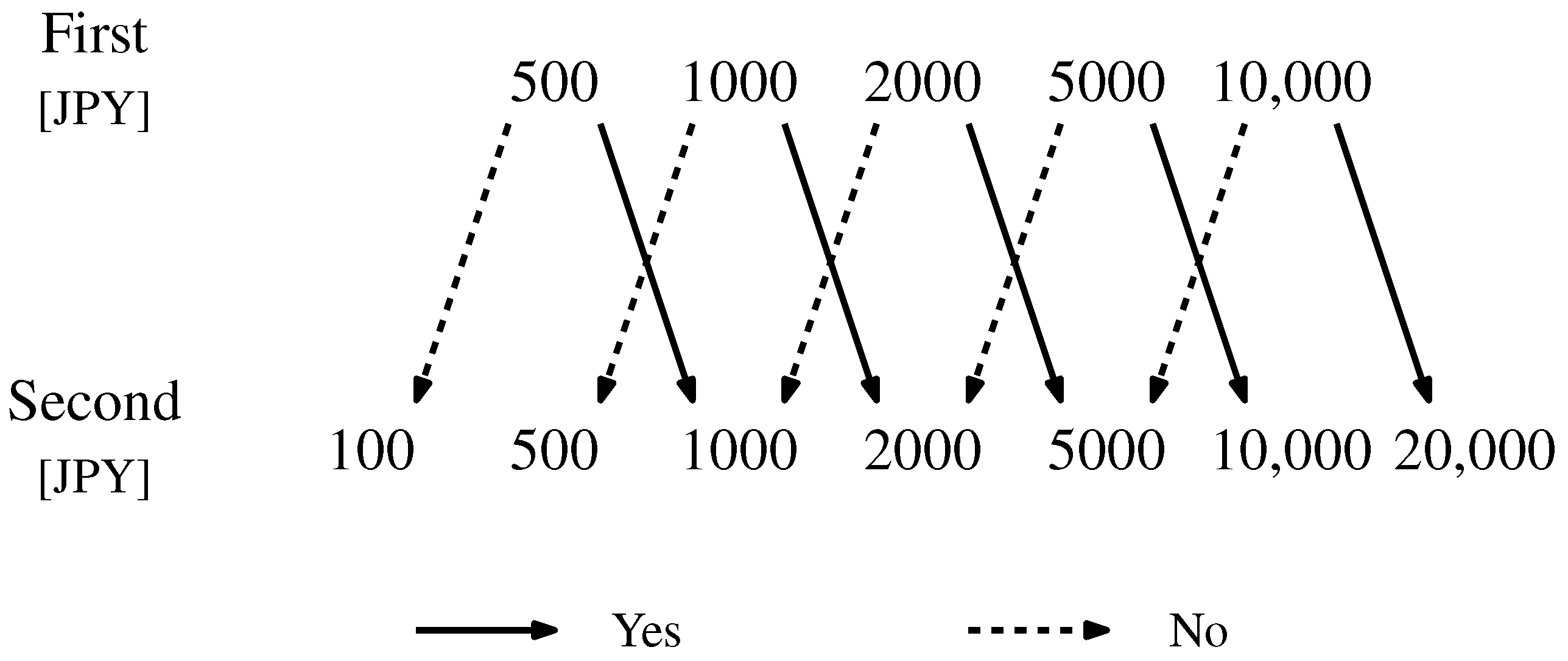
2.2. Contingent Valuation Method

This paper estimates residential VoLL using the contingent valuation method (CVM). The CVM is one of the stated preference methods used to estimate the value of goods not exchanged in the market. This paper follows the methodology explained in the previous report and survey [29,30]. The survey was conducted online to ask about willingness to pay (WTP) for a hypothetical service that avoids an outage for residential respondents. The answers are aggregated to quantify the representative value and the distribution of residential VoLL.

The WTP to prevent an outage depends on the outage situation. The survey introduces a hypothetical outage situation before the WTP question. In this situation, the outage happens at 14:00 on a summer day and continues for 2 h. Respondents are presented with two outage cases that are different in terms of the predictability of the outage. In Case 1, the outage occurs due to a rolling blackout announced one day before. In Case 2, the unpredictable outage occurs via an earthquake. Gas and water supplies are assumed to not be interrupted during the outage.

The survey introduces the hypothetical service to avoid an outage, as stated below.

“Assume that there is the following paid service for households to keep power supply during the outage. This special supply service allows customers to use electricity during the outage by paying a fee. The fee is paid after each outage, separately from the electricity bill.”

Then, the survey asks about the WTP for this service. The survey also notifies respondents that their money would decrease if they paid for the service, bringing their budget to mind.

The survey inquires about WTP using the double-bounded dichotomous method [29]. The respondents answered twice whether or not they would pay the presented price. After the first answer, the same question is asked again but with a different price. The second presented price depends on the first answer. It is higher than the first one when the first answer is “willing to pay” (yes) and is lower when the first answer is “not willing to pay” (no). Figure 1 shows the options for the prices presented. The first price is chosen randomly. It is the same in both outage cases and for each respondent. The two answers narrow the range of respondents’ WTP (e.g., the first price is 500 JPY, and the respondent answers yes and then no; the WTP is from JPY 500 to JPY 1000).

The first answer includes yes, no, and a third option: “not using”, meaning that the respondent does not want to use the service. This differs from “not willing to pay” (no), meaning the respondent wants to use it but thinks the service is expensive. The third option detects resistive answers combined with the reason for choosing it [29,30].

The options for the reasons are stated below:

• I have already prepared against a 2 h power outage;
• I will not be troubled during a 2 h power outage;
• I do not want to pay any fees for this service;
• Power outages should be avoided by power companies;
• Other.

When the respondent chooses “Others”, concrete reasons are written in a blank space. Figure 2 shows the categorization of the “not using” answers according to their reasons. Resistive answers demonstrate a payment rejection not for economic reasons but discontent with hypothetical situations or payment methods. The third and fourth reasons are considered resistive. Free answers can be resistive when they do not demonstrate economic reasons. The first reason is not resistive, but it demonstrates that respondents have already paid for equipment to prevent outages. It can cause underestimation in terms of WTP to prevent outages. Thus, these answers are excluded from VoLL estimation. Answers using the second reason and part of the freeform answers can be included in the estimation.

2.3. Estimation Model

The outage cost differs in various households, which can be modeled as a probability distribution. This paper uses the random utility model to explain the decision to pay for the outage prevention service. In this model, people accept to pay for the service when their utility when using the service is higher than without it. Utility is divided into decisive and error terms, as shown in (1). T denotes the service fee. V denotes the decisive term, which explains the effect of the service fee asked in the questionnaire. $\epsilon$ denotes the error term, which explains the other factors. In this paper, $\epsilon$ follows a Gumbel distribution. The distribution function of the Gumbel distribution is written in (2).

$$\begin{array}{cc}\hfill U\left(T\right)& =V\left(T\right)+\epsilon \hfill \end{array}$$

(1)

$$\begin{array}{cc}\hfill F\left(\epsilon \right)& =exp\left(-exp(-\epsilon )\right)\hfill \end{array}$$

(2)

Whether or not to pay for the service depends on the utility difference with and without the service. If utility with the service minus utility without it is positive, people are willing to pay. The utility difference follows a log-linear function with the service fee, as shown in (3). $\gamma$ and ${\beta }_0$ denote coefficients. The probability of paying for the service using price T follows a logistic function, as shown in (4). The coefficients $\gamma$ and ${\beta }_0$ are estimated using the maximum likelihood method. The answers in the survey specify the range of the respondent’s WTP. On the other hand, the probability that WTP falls into each range can be calculated using (4). Thus, the likelihood of each answer can be calculated.

$$\begin{array}{cc}\hfill & \begin{array}{cc}\hfill \Delta V\left(T\right)& =V\left(T\right)-V\left(0\right)\hfill \\ \hfill & =-\gamma logT-{\beta }_0\hfill \end{array}\hfill \end{array}$$

(3)

$$\begin{array}{cc}\hfill & \begin{array}{cc}\hfill \mathrm{Prob}[\mathrm{WTP}>T]& =\mathrm{Prob}[{\epsilon }_0<\Delta V\left(T\right)+{\epsilon }_1]\hfill \\ \hfill & ={\displaystyle \frac{exp(\gamma logT+{\beta }_0)}{1+exp(\gamma logT+{\beta }_0)}}\hfill \end{array}\hfill \end{array}$$

(4)

After estimating the coefficients, their significance is tested by the Wald test [31].

The Wald test assumes a distribution of the difference between the estimated and true coefficients as a normal distribution. The null hypothesis is that the coefficients are zero. The test statistic is the square of the tested coefficients normalized by their estimated variance. The Hessian of log-likelihood calculates the estimated variance. The test statistic follows a chi-squared distribution. Its degree of freedom equals the number of coefficients the null hypothesis affects. The test is the same as the t-test when the degree of freedom is 1. The set of tested coefficients is significant if the test statistic is large enough to be in the critical region with a particular significance level.

3. Value of Lost Load Estimation

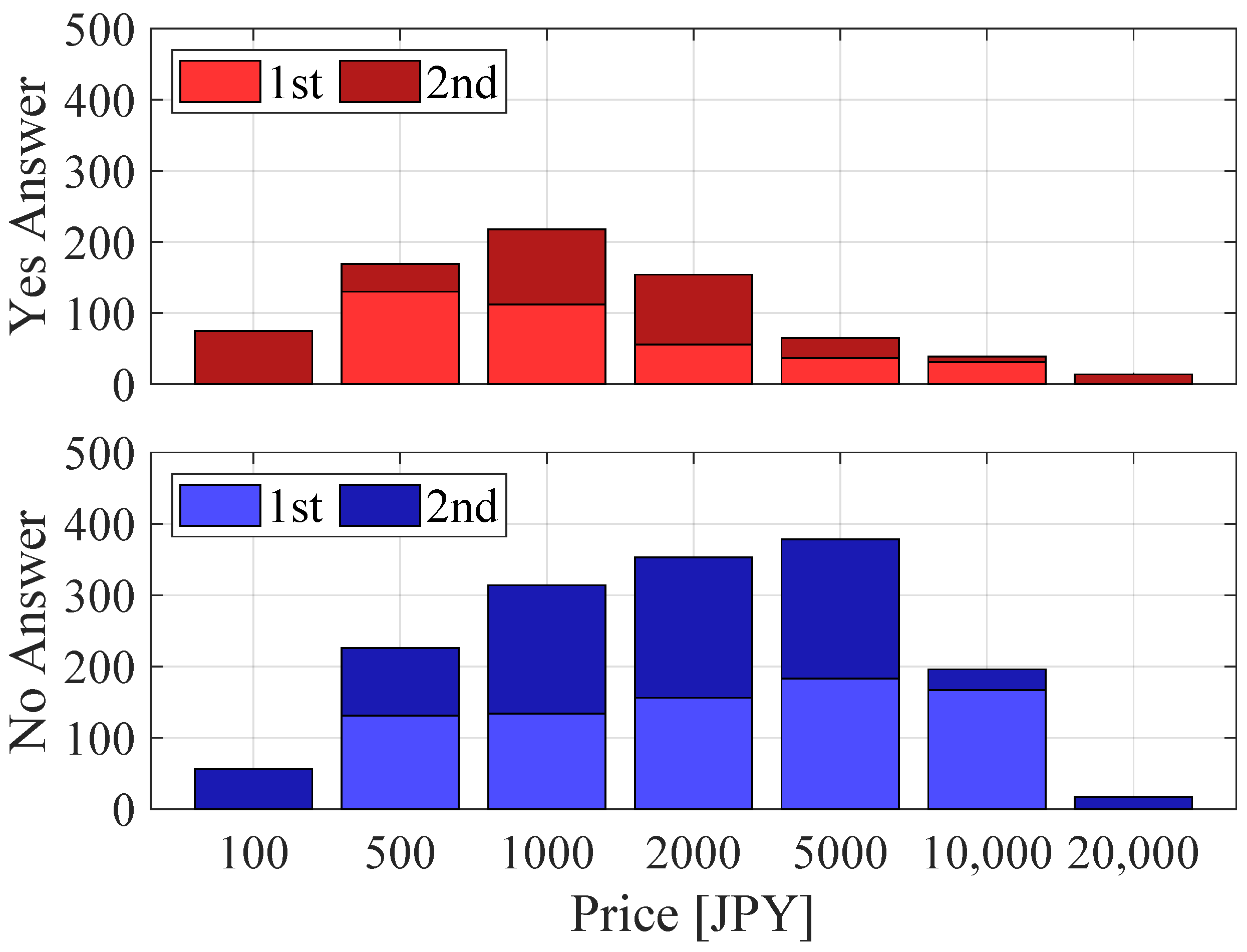
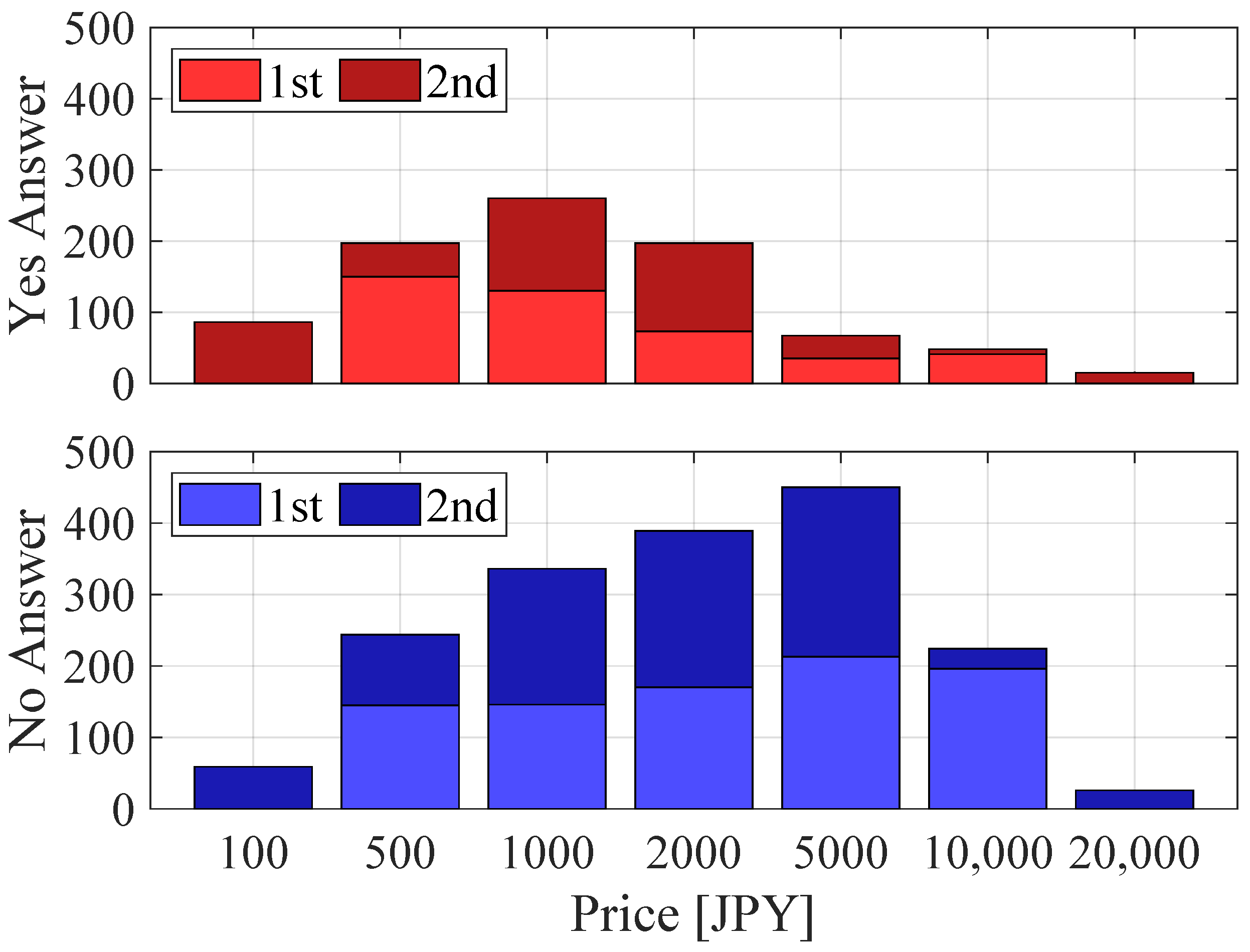
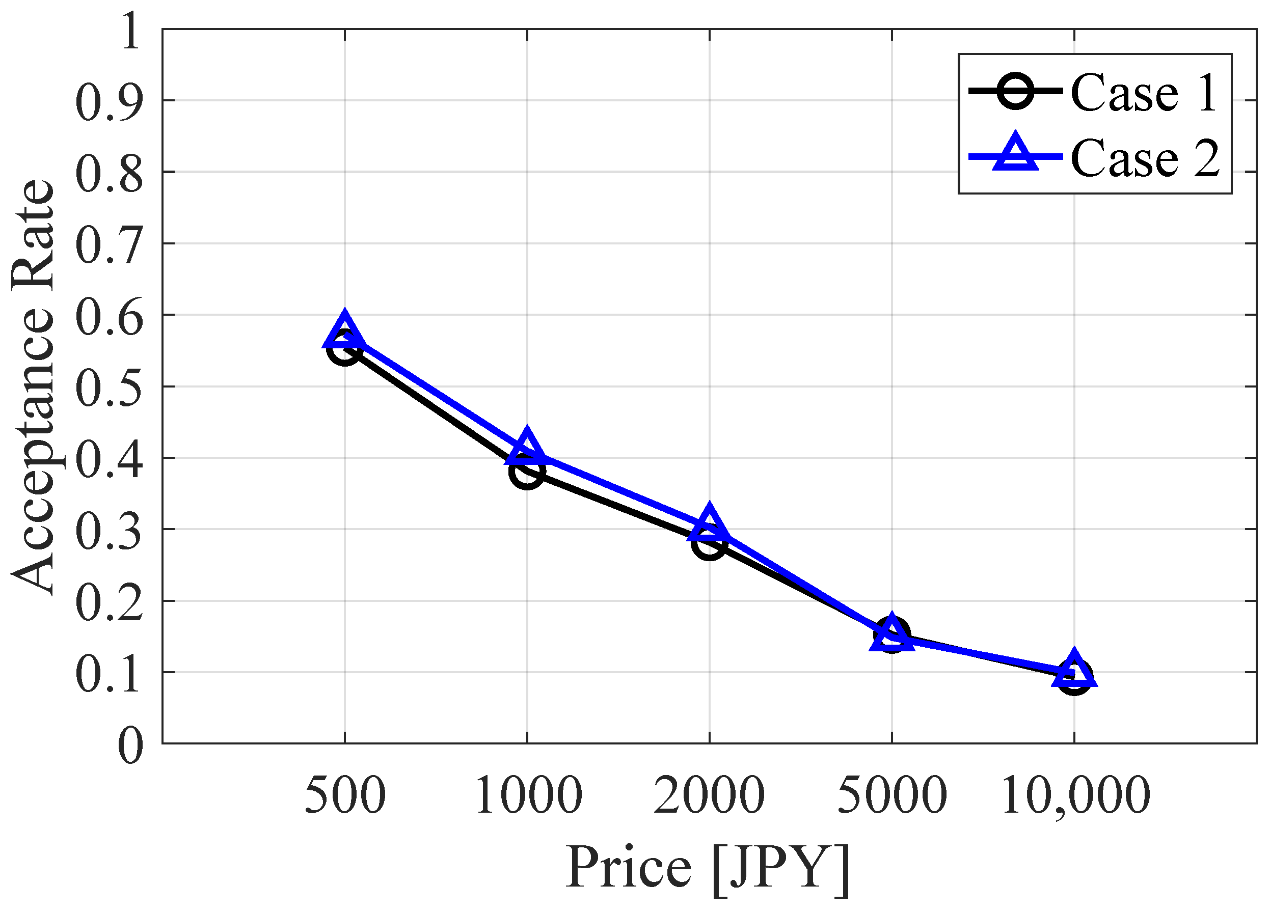
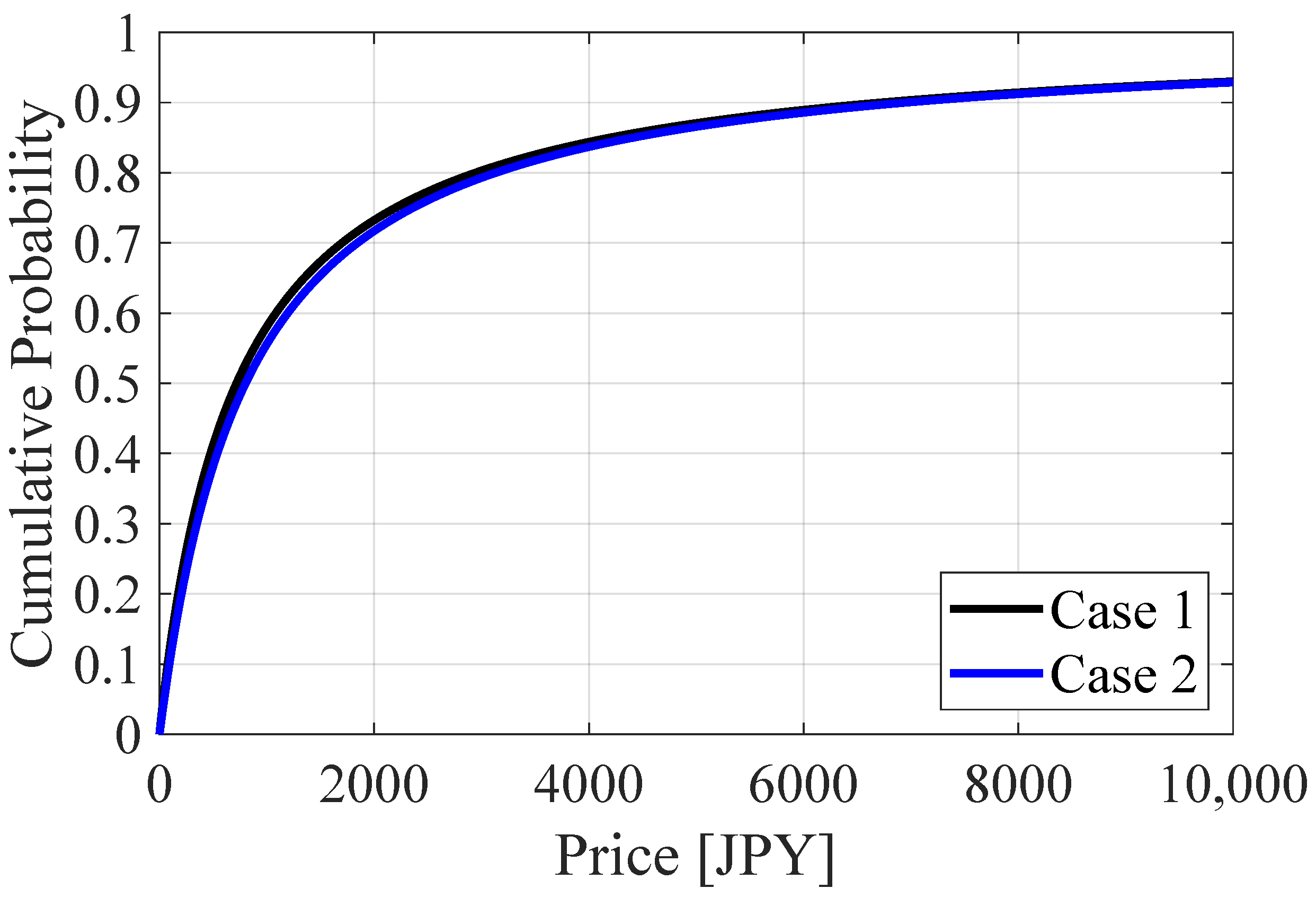
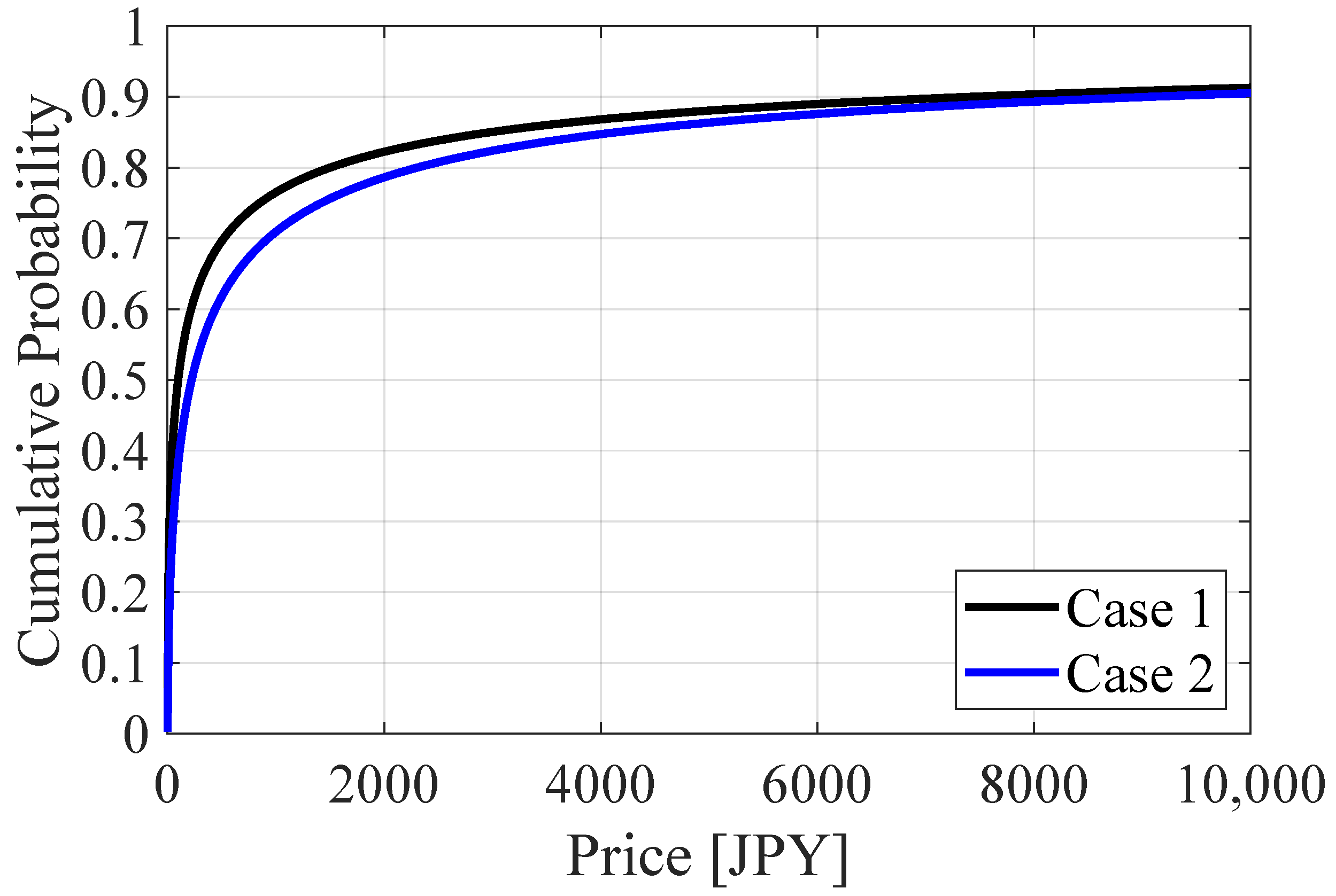
3.1. Answers of Willingness to Pay

The survey was conducted online in October 2022 with the support of a market research company. The questionnaire was sent to households in the Tokyo and Kinki areas. Around 1000 answers were collected from each area, with 2131 answers in total. All respondents were aware of their monthly electricity bills. The survey first inquired about the respondents’ basic attributes. Around half of the respondents lived in an apartment, and the others lived in detached houses. In addition, 285 respondents were in a fully electrified house.

Online surveys tend to collect answers from people who are familiar with technology [29]. This may bias the estimation.

This paper first distinguishes answers of yes and no from “not using”. The number of “not using” answers differed in each outage case. There were 994 answers (46.6%) in Case 1 and 832 (39.0%) in Case 2.

In addition, 434 answers in Case 1 and 409 in Case 2 were considered resistive. A total of 93 answers in Case 1 and 91 in Case 2 showed that the respondents had already prepared for outages. This paper uses the expression “not using” in the answers.

This means that the “not using” answers in the first question reflected residents who are not resistive and not prepared for outages. This paper considers these answers to mean that they are not willing to pay against the lowest price (JPY 100 ).

Parameter estimation is solved by using the “fminunc” function in the Optimization Toolbox of MATLAB R2024b [32]. The initial parameters given to “fminunc” were $\gamma =-$1 and ${\beta }_0$ = 4. The Wald tests were implemented in MATLAB R2024b. The program was executed using a laptop PC with Intel(R) Core(TM) i7-1260P @ $2.10$ GHz and $16.0$ GB RAM @ 4800 MHz, manufactured by Dynabook in Tokyo, Japan. It took $2.4$ s to finish the estimation using the plugged-in laptop. It took $0.17$ s to finish the Wald tests for all variables.

First, we tabulated the answers and then drew an acceptance rate curve. Figure 3 and Figure 4 show the number of answers in Cases 1 and 2 at each price. The number of “No” (“not willing to pay”) answers is higher than “Yes” (“willing to pay”) at all prices except JPY 100. The ratio of “No” increases with price in both cases. Figure 5 shows the acceptance rate curve. The acceptance rate decreases with price in both cases. The median WTP can be seen to be between JPY 500 and JPY 1000 when using this curve.

Next, we applied the logit model to the survey results. Figure 6 and Figure 7 show the distribution function of the acceptance rate from the logit model, excluding and including the “not using” answers, respectively. The plots show that the rate of WTP is lower than T [$\mathrm{JPY}$]. The acceptance rate in Case 2 is lower than in Case 1 at the same price. Their difference is less than 5% points. Excluding the “not using” answers shifts the distributions to the left.

Table 1. Fitting results for the logit model when excluding the “not using” answers.

	Case 1	Case 2
Number of samples	1137	1299
Log likelihood	−1371.8	−1584.7
$\gamma$ (t value)	−0.9821 (−25.44)	−1.0175 (−27.72)
${\beta }_0$ (t value)	6.4580 (23.20)	6.8038 (25.52)
Median of WTP [$\mathrm{JPY}$]	717.6	801.8

and

Table 2. Fitting results for the logit model when including the “not using” answers.

	Case 1	Case 2
Number of samples	1604	1631
Log likelihood	−1894.9	−2053.4
$\gamma$ (t value)	−0.5083 (−24.84)	−0.5931 (−27.68)
${\beta }_0$ (t value)	2.3304 (17.10)	3.2052 (21.68)
Median of WTP [$\mathrm{JPY}$]	98.0	222.4

show the parameters in the logit model and the median WTP value when excluding and including the “not using” answers, respectively. The coefficient of the prices $\gamma$ is negative and significant in all cases. This means that fewer people accept higher prices to avoid outages. The median of WTP is JPY 700–800 when excluding the “not using” answers. This matches the result from the acceptance rate curve (Figure 5). The median WTP when including the “not using” answers is one-seventh lower than when excluding them because around 25% of the valid answers are “not using”.

This paper excludes the “not using” answers when they are paired with the reason of already being prepared for outages. The estimated parameters of the logit models change when these answers are included. This shows a sensitivity analysis for WTP estimation based on the logit model. The answer of not willing to pay against the lowest price (JPY 100) increased by 93 (Case 1) and 91 (Case 2). In Case 1, the estimated parameters are $\gamma =-0.4818$ and ${\beta }_0=2.0503$. In Case 2, the estimated parameters are $\gamma =-0.5511$ and ${\beta }_0=2.8053$. Both $\gamma$ and ${\beta }_0$ are lower than in Table 2 in Cases 1 and 2. The median of WTP is JPY 70.5 (Case 1) and JPY 161.9 (Case 2). It is 22% smaller than that in Table 2.

3.2. Value of Lost Load Calculation

The WTP inquired about in the survey represents the value of preventing a 2-h outage. We converted this value into the cost per power not supplied $\mathrm{kWh}$. The representative value of WTP is defined as the median in the survey result (Table 1 and Table 2). Then, it was converted into VoLL and divided by the demand sum for 2 h.

First, this paper uses the actual demand in 70 households to calculate the summed demand for 2 h. Figure 8 shows the histogram of the demand sum for 2 h. The time range to calculate the sum is 14:00–16:00 in August. Thus, 31 data per household are included in the histogram, and there are 70 × 31 = 2170 in total. The median of the demand sums is $1.432$ kWh.

The average of the demand sum is $1.605$ kWh, which is 12% greater than the median. This paper uses the median as the representative demand during a 2 h outage.

Then, we calculated VoLL using the median values for WTP and the demand sum. From the survey, four median values for WTP were obtained for different cases and data ranges, as shown in Table 1 and Table 2. The VoLL is $68.4$ JPY/kWh (Case 1) and $155.3$ JPY/kWh (Case 2) when including the “not using” answers. In contrast, the VoLL is $501.1$ JPY/kWh (Case 1) and $559.9$ JPY/kWh (Case 2) when excluding the “not using” answers. The result values are four–eight times larger than when including the “not using” answers.

When using an average of 2 h for the demand sums, the VoLL is $447.1$ JPY/kWh (Case 1) and $499.6$ JPY/kWh (Case 2) when excluding the “not using” answers.

The estimated VoLL values show the damage in a limited situation, demonstrating a 2 h power outage from 14:00 to 16:00 during summer. The VoLL values differ with the timing and duration of power outages [9,11,16,26,27]. Macroeconomic methods imply larger VoLL values during demand peaks [26,27]. In Japan, the residential peak demand generally happens in summer. In addition, demand tends to be larger in the evening than in the daytime. In the previous survey, the VoLL in summer during daytime is around 40% higher than in winter evenings in Japan [9]. Hence, the estimated VoLL may be higher than that in other seasons but lower than that for summer evenings. In terms of outage duration, the survey in New Zealand [11] showed that outage cost increases with longer duration, but VoLL decreases. The residential VoLL of a 1 h outage in winter is twice as large as that of a 5 h outage in winter [11]. VoLL reduction decelerates with longer outages [11,16]. Thus, the estimated VoLL in this paper can be reduced to around half or less than half if an outage continues for 5 h or longer.

Finally, this paper compares the estimated VoLL to that of previous research.

Table 3. Comparison of residential VoLLs between this survey and previous research. VoLL values were converted to USD using the average exchange rates in the relevant year.

Area	Year	Method	VoLL		Ref.
Japan	2022	CVM	3.83–4.28 $\mathrm{USD}/\mathrm{kWh}$	(501–560 $\mathrm{JPY}/\mathrm{kWh}$)	This paper
Japan	1999	CVM	11.87–23.75 $\mathrm{USD}/\mathrm{kWh}$	(1350–2700 $\mathrm{JPY}/\mathrm{kWh}$)	[20]
Japan	2012	CVM	65.52 $\mathrm{USD}/\mathrm{kWh}$	(5230 $\mathrm{JPY}/\mathrm{kWh}$)	[33]
Japan	2019	CVM	39.60–74.47 $\mathrm{USD}/\mathrm{kWh}$	(4317–8118 $\mathrm{JPY}/\mathrm{kWh}$)	[9]
Korea	2015	CVM	2.75–3.45 $\mathrm{USD}/2\mathrm{h}$	(3103–3900 $\mathrm{KRW}/2\mathrm{h}$)	[21]
US	2020	CVM	1.8–2.2 $\mathrm{USD}/\mathrm{kWh}$		[17]
Australia	2014	CVM	32.55 $\mathrm{USD}/\mathrm{kWh}$		[14]
UK	2018	CVM	2.67 $\mathrm{USD}/\mathrm{kWh}$	(2 $\mathrm{GBP}/\mathrm{kWh}$)	[10]
New Zealand	2018	CVM	11.75–27.64 $\mathrm{USD}/\mathrm{kWh}$	(17–40 $\mathrm{NZD}/\mathrm{kWh}$)	[11]
Italy	2022	CVM	7.88 $\mathrm{USD}/\mathrm{kWh}$	(7.5 $\mathrm{EUR}/\mathrm{kWh}$)	[16]
Japan	1999	Macroeconomic	21.19 $\mathrm{USD}/\mathrm{kWh}$	(2409 $\mathrm{JPY}/\mathrm{kWh}$)	[20]
Netherlands	2007	Macroeconomic	22.44 $\mathrm{USD}/\mathrm{kWh}$	(16.38 $\mathrm{EUR}/\mathrm{kWh}$)	[26]
Norway	2011	Macroeconomic	34.19 $\mathrm{USD}/\mathrm{kWh}$	(24.6 $\mathrm{EUR}/\mathrm{kWh}$)	[34]
Cyprus	2012	Macroeconomic	11.70 $\mathrm{USD}/\mathrm{kWh}$	(9.07 $\mathrm{EUR}/\mathrm{kWh}$)	[28]
Portugal	2016	Macroeconomic	8.25 $\mathrm{USD}/\mathrm{kWh}$	(7.43 $\mathrm{EUR}/\mathrm{kWh}$)	[27]

shows the areas, years, methods, and residential VoLLs from the relevant research. All VoLL values are converted to USD, but they cannot be directly compared to the result in this paper because the VoLL values differ according to different economies, cultures, and power reliability. The VoLL in this paper is relatively small compared to other papers. In Japan, the estimated residential VoLLs when using the CVM are much higher than those of this paper. For example, the result in [9] shows over 10 times higher VoLL values.

4. Attributes Effects

4.1. Random Utility Model with Attributes

In addition to asking about WTP, the survey also inquired about the attributes of the respondents.

Table 4. Questions and choices relating to the attributes in the survey. Choices in italics regarding the attributes used in the random utility model are excluded.

Question	Choice
Occupation	Office worker/Self-employment/ Part-time/Student/Homemaker/ Unemployed/Other
Address	Kanto/Kinki
House type	Apartment/Detached
Fully-electrified house	Yes/No
Monthly electricity bill	JPY 0–2000/JPY 2000–4000/ JPY 4000–7000/JPY 7000–10,000/ JPY 10,000–15,000/JPY 15,000–20,000/ >JPY 20,000
Blackout experienced after 2018	Yes/No
Number of blackouts experienced	1 or 2/3 or 4/5 or 6/7 or more
Evacuation experienced after 2018	Yes/No/No disaster experience
Place where you evacuated to	Public evacuation shelter/ Hotel/Relatives’ house/Other
Willingness to evacuate	Yes/No/Don’t know
Place where you will evacuate to	Public evacuation shelter/ Hotel/Relatives’ house/Other
Damage experienced from the disaster	Gas interruption/ Water interruption/ Stop cooking appliances/ Stop boiling water/ Stop warming room/Nothing
Having stockpiles	Yes/No
Stockpile amount	1 day/2 or 3 days/ 4–6 days/7 days or more
Capacity of mobile battery you have	Don’t have / <3 Ah/3–6 Ah/6–10 Ah / 10–20 Ah/>20 Ah/Don’t know
Have known “power supply alert”	Yes/No
Have known “power supply caution”	Yes/No
Willingness to buy stockpiles if notifying rolling blackout	Yes/No/Don’t know
Household annual income **	< JPY 2 M * /JPY 2 M–3 M/ JPY 3 M–4 M/JPY 4 M–6 M/ JPY 8 M–10 M/JPY 10 M–20 M/ >JPY 20 M/Don’t know
Hours at home on weekdays	0–3 h/3–6 h/ 6–9 h/>9 h/Don’t know
Power generating equipment in your house	Solar panel/Co-generating system/ Fossil fuel generator/Static battery/ Nothing

* M denotes million (JPY). ** The choice of JPY 6 M–8 M is not included by mistake.

shows the list of the questions and choices. The attributes include respondents’ occupation, monthly electricity bill, housing type, income, experience with outages, and experience with evacuation during disasters.

The random utility model can evaluate the effect of the attributes on WTP. This paper includes attributes to express the difference in the utility’s decisive terms (V). The difference $\Delta V$ is shown in (5). $\mathbf{x}$ denotes a person’s attribute vector. $\gamma$ and $\mathsf{\beta }$ denote the coefficients of the service price T and the attributes $\mathbf{x}$. ${\beta }_0$ denotes a constant.

The elements of $\mathbf{x}$ are binary, corresponding to the choices in the survey. A variable becomes 1 if the respondent selects the corresponding choice. The questions shown in Table 4 have multiple-choice answers. Thus, one of the elements corresponding to one question must be 1, and the others must be 0. One of the choices of each question is excluded in the elements of $\mathbf{x}$ to avoid collinearity.

This paper used all the questions in Table 4 in the model to find significant attributes.

The probability of paying for the service for price T is calculated in (6). The coefficients $\gamma ,\mathsf{\beta }$, and ${\beta }_0$ are estimated using the maximum likelihood method. The answers using attributes were used to calculate the likelihood. The significance of the attributes was tested using the Wald test.

$$\begin{array}{cc}\hfill & \begin{array}{cc}\hfill \Delta V(T,\mathbf{x})& =V(T,\mathbf{x})-V(0,\mathbf{x})\hfill \\ \hfill & =-\gamma logT-\mathsf{\beta }\mathbf{x}-{\beta }_0\hfill \end{array}\hfill \end{array}$$

(5)

$$\begin{array}{cc}\hfill & \mathrm{Prob}[{\mathrm{WTP}}_{\mathbf{x}}>T]={\displaystyle \frac{exp(\gamma logT+\mathsf{\beta }\mathbf{x}+{\beta }_0)}{1+exp(\gamma logT+\mathsf{\beta }\mathbf{x}+{\beta }_0)}}\hfill \end{array}$$

(6)

Parameter estimation using the maximum likelihood method is solved by using the same environment shown in Section 3.1. The initial parameters given to “fminunc” were $\gamma =-$1, ${\beta }_0=$ 4, and 0.01, as was the same for other coefficients ($\mathsf{\beta }$). It took 264 s to finish the estimation using the plugged-in laptop.

4.2. Result

The effect of the attributes was analyzed using WTP and the attributes. The analysis excludes the “not using” answers to avoid distortion from many of the lowest WTP values.

Table 5. Fitting results for the random utility model with attributes. The attribute results are excluded from the table values.

	Case 1	Case 2
Number of samples	1137	1299
Log likelihood	−1305.4	−1499.9
$\gamma$ (t value)	−1.0679 (−24.60)	−1.1206 (−27.46)
${\beta }_0$ (t value)	5.3226 (15.90)	7.4426 (20.52)

shows the overall estimation result from the random utility model using the attributes. The t-values of the coefficient of prices ($\gamma$) and the constant are far from zero; this shows their significance in the model. The price coefficient is negative, the same as the estimation without the attributes. In addition, the null hypothesis that all coefficients of the attributes ($\mathsf{\beta }$) are zero is rejected, with a p-value of less than 10⁻⁴. Thus, not only the service price but also the attributes affect WTP.

Next, this paper investigates the significance of each attribute.

It can be noticed that the attributes ($\mathbf{x}$) have weak correlations with each other.

Table 6. Significant questions and their p-values in Cases 1 and 2.

Question	Deg. of Freedom	p-Value in Case 1	p-Value in Case 2
Occupation	6	0.3420	0.0722 *
Monthly electricity bill	6	0.0043 ***	0.0211 **
Blackout experience	1	0.0498 **	0.1026
Evacuation experience	2	0.4593	0.0132 **
Willingness to evacuate	2	0.0455 **	0.0916 *
Damage experience	5	0.0683 *	0.2551
Having stockpiles	1	0.0765 *	0.0509 *
Stockpile amount	3	0.3949	0.0982 *
Willingness to buy stockpiles	2	0.1397	0.0099 ***
Household annual income	7	2.9772 × 10−4 ***	6.3009 × 10−6 ***
Power generating equipment	4	0.2758	0.0122 **

* Reject the null hypothesis at the 10% significance level. ** Reject the null hypothesis at the 5% significance level. *** Reject the null hypothesis at the 1% significance level.

shows the significant questions and their p-values in Cases 1 and 2. The degrees of freedom value equals the number of choices in the question minus 1.

p-values were calculated using the Wald test statistics.

The factors of monthly electricity bill, willingness to evacuate, stockpiles, and annual income are significant in both cases. Thus, these attributes affected WTP to avoid a 2 h outage, whether the outage was predictable or not. The questions about stockpiles and generating equipment are significant only in Case 2. The outage in Case 2 suddenly happens due to earthquakes. The respondents who have stockpiles and generation equipment can be sensitive to such sudden disasters. Thus, those attributes have an effect only in Case 2.

This paper also investigates the significance of each choice. Each choice corresponds to each variable in the model.

Table 7. Coefficients, p-values, and the number of answers of significant variables in Case 1.

Variable	Coefficient	p-Value	Num.
Monthly electricity bill: JPY 15,000–20,000	1.6649	0.0822 *	157
Evacuation experience: Yes	0.3282	0.0498 **	312
Place where you evacuated: Public evacuation shelter	2.2683	0.0759 *	12
Willingness to evacuate: Yes	0.5019	0.0135 **	218
Damage experience by disaster: Stop cooking appliances	−0.7242	0.0454 **	84
Having stockpiles: Yes	0.5679	0.0765 *	725
Household annual income: JPY 2 M–3 M	0.7322	0.0205 **	86
Household annual income: JPY 3 M–4 M	0.7422	0.0105 **	131
Household annual income: JPY 4 M–6 M	0.5744	0.0209 **	341
Household annual income: JPY 8 M–10 M	0.7570	0.0041 ***	206
Household annual income: JPY 10 M–15 M	1.0187	0.0002 ***	158
Household annual income: JPY 15 M–20 M	1.4778	0.0057 ***	19
Power generating equipment: Solar panel	−0.5214	0.0959 *	68
Power generating equipment: Co-generating system	0.6496	0.0990 *	32

* Reject the null hypothesis at the 10% significance level. ** Reject the null hypothesis at the 5% significance level. *** Reject the null hypothesis at the 1% significance level.

and

Table 8. Coefficients, p-values, and the number of answers of significant variables in Case 2.

Variable	Coefficient	p-Value	Num.
Occupation: Student	1.5288	0.0648 *	8
Monthly electricity bill: JPY 2000–4000	−1.1331	0.0944 *	94
Blackout experienced times: 5 or 6	−1.4763	0.0942 *	9
Evacuation experience: No	−0.8353	0.0044 ***	1216
Willingness to evacuate: Yes	0.3664	0.0493 **	252
Damage experience by disaster: Stop cooking appliances	−0.6356	0.0477 **	100
Having stockpiles: Yes	0.5423	0.0509 *	829
Stockpile amount: 7 days or more	−0.7061	0.0380 **	93
Willingness to buy stockpiles: Yes	0.5937	0.0082 ***	445
Household annual income: JPY 3 M–4 M	0.6282	0.0212 **	145
Household annual income: JPY 4 M–6 M	0.6428	0.0062 ***	389
Household annual income: JPY 8 M–10 M	0.7970	0.0012 ***	243
Household annual income: JPY10 M–20 M	1.1281	<10−4 ***	165
Household annual income: >JPY 20 M	1.7629	0.0006 ***	21
Power generating equipment: Co-generating system	0.8581	0.0184 ***	40
Power generating equipment: Fossil fuel generator	2.5232	0.0148 ***	6

* Reject the null hypothesis at the 10% significance level. ** Reject the null hypothesis at the 5% significance level. *** Reject the null hypothesis at the 1% significance level.

show the significant variables in Cases 1 and 2, respectively.

These tables include the coefficients ($\mathsf{\beta }$ in equation (5)), p-values, and numbers of corresponding answers in the survey. The p-values were calculated using the Wald test statistics.

A positive coefficient means that the variable or the attribute increases WTP. In both cases, annual income significantly increased WTP. In addition, WTP tends to increase with annual income. This implies that people who have higher incomes can afford to pay higher service prices. The willingness to evacuate also significantly increases WTP in both cases. This reflects anxiety about disasters, which influences WTP. In Case 2, having many stockpiles decreases WTP, and the willingness to buy stockpiles increases it. These relationships reflect feelings of security and anxiety about disasters, respectively. Having power-generating equipment increases WTP, except for solar panels. This also relates to anxiety about disasters. However, the equipment can generate electricity even during outages. The relationship implies that the respondents might not have known that their equipment could work during outages. Finally, the experience of damage on cooking appliances significantly decreases the WTP. Most respondents who experienced damage to cooking appliances also had stockpiles. Thus, they may not have felt anxiety about the short-term outage. In Case 2, over 90% of respondents answered they had no experience with evacuation. It significantly decreases WTP. This can imply that the experience of other disasters without evacuation makes them confident of surviving short outages. However, the significance of this choice might be indirectly affected by other attributes because of many answers.

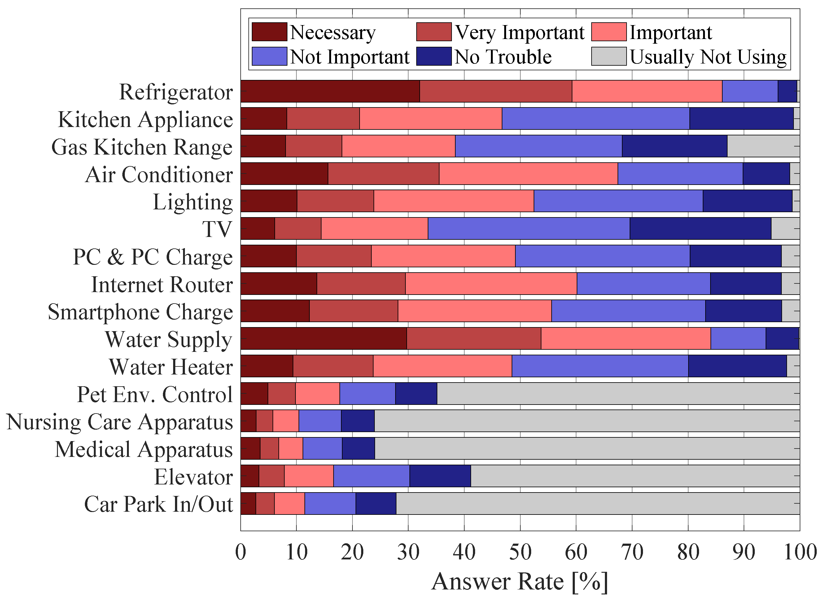
5. Load Importance During Outages

The survey also asked respondents about the importance of electric loads in Cases 1 and 2 after the question about their WTP. The importance of 16 different types of loads during the outage was inquired about. The loads include appliances for daily use (e.g., refrigerator, kitchen appliances, and smartphone charge), electricity use to supply water, and critical use (e.g., medical apparatus). The choices are based on a five-point Likert scale. In addition, the option of not using the load regularly (“Usually Not Using”) is included.

The answers regarding the importance of loads in Cases 1 and 2 are shown in Figure 9 and Figure 10, respectively. The most important loads are refrigerators and water supplies. Around 80% of the respondents answered they were necessary, very important, or important. The second-most important load is air conditioners. Around 70% of the respondents answered that it was necessary, very important, or important. In contrast, most respondents did not regularly use environmental control for pets, nursing care and medical apparatus, elevators, and car parking. The result demonstrates that nursing care and medical apparatus are not so important.

Around 25% of respondents regularly use nursing care and medical apparatus.

The rate of the answer that they are important is less than 50%, even when “Usually Not Using” is excluded.

The survey inquired about the importance of nursing care and medical apparatus without specifying their usage. This general form of questioning may have led some respondents to imagine medical usages that were not critical for life. Thus, the survey may underestimate the importance of nursing care and medical apparatus during outages. Respondents can answer more precisely about the importance of nursing care and medical apparatus if the questionnaire specifies concrete usages, such as electric wheelchairs and oxygen supplies.

6. Conclusions

Recently, measures against supply shortages caused by disasters have become more important. Estimating the value of lost loads (VoLLs) helps to create optimal measures. This paper aimed to investigate the current residential VoLL in Japan by using a survey. Residential VoLL was estimated using residents’ willingness to pay (WTP) to avoid power outages. The median WTP to prevent a 2 h outage in the summer is JPY 717.6 in a predictable outage and JPY 801.8 in a sudden outage. WTP was converted into residential VoLL by using actual demand. The VoLL is $501.1$ JPY/kWh in a predictable outage and $559.9$ JPY/kWh in a sudden outage. Next, we used a random utility model and Wald testing to analyze the relationship between WTP and people’s attributes. As a result, it was found that the annual income of households and electricity bills significantly affect WTP. Evacuation experiences and stockpiles also affect the WTP to avoid a sudden outage. Finally, this paper investigated the importance of each load in households. A total of 80% of respondents answered that refrigerators, air conditioners, and water supplies are important. In contrast, around half of respondents think other loads are unimportant.

In the survey, some questions on load importance and usage are unclear; this may underestimate the importance of some critical loads, especially medical usage. In addition, there are around 400 resistive answers in the WTP inquiry, which is larger than the survey in Norway [18]. The number of resistive answers may be reduced by providing details about the damage caused by power outages. The survey is a first step toward investigating residential VoLL and load importance. Future surveys will be carried out to formulate more specific representations.

In addition, the survey used in this paper inquires about WTP in situations where an outage occurs during the daytime in summer and continues for 2 h.

Future work will collect data for various outage situations.

References

1. Busby, J.W.; Baker, K.; Bazilian, M.D.; Gilbert, A.Q.; Grubert, E.; Rai, V.; Rhodes, J.D.; Shidore, S.; Smith, C.A.; Webber, M.E. Cascading risks: Understanding the 2021 winter blackout in Texas. Energy Res. Soc. Sci. 2021, 77, 102106. [Google Scholar] [CrossRef]
2. Cabinet Office Japan. White Paper on Disaster Management 2020: Special Feature: Catastrophic and Frequent Torrential Rain. 2020. Available online: https://www.bousai.go.jp/en/documentation/white_paper/pdf/2020/SF1-1.pdf (accessed on 4 March 2025).
3. Cabinet Office Japan. White Paper on Disaster Management 2019: Special Feature: Consecutive Disasters—Toward the Establishment of a Disaster Conscious Society. 2019. Available online: https://www.bousai.go.jp/en/documentation/white_paper/pdf/SF1-1.pdf (accessed on 4 March 2025).
4. de Nooij, M.; Lieshout, R.; Koopmans, C. Optimal blackouts: Empirical results on reducing the social cost of electricity outages through efficient regional rationing. Energy Econ. 2009, 31, 342–347. [Google Scholar] [CrossRef]
5. Ovaere, M.; Heylen, E.; Proost, S.; Deconinck, G.; Hertem, D.V. How detailed value of lost load data impact power system reliability decisions. Energy Policy 2019, 132, 1064–1075. [Google Scholar] [CrossRef]
6. Xiang, T.; Li, P.; Wang, G.; Wang, N.; Fan, X.; Zhao, Y. Reliable Electricity Pricing Method of Distribution Network Considering Outage Loss Increment and Differentiated Demand. In Proceedings of the 2021 IEEE 5th Conference on Energy Internet and Energy System Integration (EI2), Taiyuan, China, 22–24 October 2021; pp. 3564–3569. [Google Scholar] [CrossRef]
7. Uthathip, N.; Bhasaputra, P.; Pattaraprakorn, W. Outage Cost Assessment for Investment-Benefit Model of Smart Grid in Thailand. In Proceedings of the 2016 International Conference on Cogeneration, Small Power Plants and District Energy (ICUE 2016), Bangkok, Thailand, 14–16 September 2016; pp. 1–5. [Google Scholar]
8. Safamanesh, A.; Ghaziziadeh, M.S.; Habibi, M.; Vahidinasab, V. Sustainable and Inclusive Demand-Side Resilience: A Semi-Dynamic Model for Outage Costs. In Proceedings of the 2023 IEEE PES GTD International Conference and Exposition (GTD), Istanbul, Turkiye, 22–25 May 2023; pp. 166–170. [Google Scholar] [CrossRef]
9. Organization for Cross-Regional Coordination of Transmission Operators. Technical Scrutiny of Outage Costs (in Japanese). 2019. Available online: https://www.occto.or.jp/iinkai/kouikikeitouseibi/resilience/2018/files/resilience_04_03_01.pdf (accessed on 4 March 2025).
10. Electricity North West. The Value of Lost Load. 2018. Available online: https://www.enwl.co.uk/globalassets/innovation/enwl010-voll/voll-general-docs/voll--summary-factsheet.pdf (accessed on 4 March 2025).
11. Transpower New Zealand Limited. Value of Lost Load Study. 2018. Available online: https://static.transpower.co.nz/public/publications/resources/Value%20of%20Lost%20Load%20%28VoLL%29%20Study%20-%20June%202018.pdf (accessed on 4 March 2025).
12. Willis, K.; Garrod, G. Electricity supply reliability: Estimating the value of lost load. Energy Policy 1997, 25, 97–103. [Google Scholar] [CrossRef]
13. Jha, D.K.; Sinha, S.K.; Garg, A.; Vijay, A. Estimating electricity supply outage cost for residential and commercial customers. In Proceedings of the 2012 North American Power Symposium (NAPS), Champaign, IL, USA, 9–11 September 2012; pp. 1–6. [Google Scholar] [CrossRef]
14. Hensher, D.A.; Shore, N.; Train, K. Willingness to pay for residential electricity supply quality and reliability. Appl. Energy 2014, 115, 280–292. [Google Scholar] [CrossRef]
15. Morrissey, K.; Plater, A.; Dean, M. The cost of electric power outages in the residential sector: A willingness to pay approach. Appl. Energy 2018, 212, 141–150. [Google Scholar] [CrossRef]
16. Marchisio, L.; Genoese, F.; Vedovelli, F.; Salterini, F.; Costa, S. Estimating the Value of Lost Load in Italy through outage cost surveys. In Proceedings of the 2022 AEIT International Annual Conference (AEIT), Rome, Italy, 3–5 October 2022; pp. 1–5. [Google Scholar] [CrossRef]
17. Baik, S.; Davis, A.L.; Park, J.W.; Sirinterlikci, S.; Morgan, M.G. Estimating what US residential customers are willing to pay for resilience to large electricity outages of long duration. Nat. Energy 2020, 5, 250–258. [Google Scholar] [CrossRef]
18. Vennemo, H.; Rosnes, O.; Skulstad, A. The cost to households of a large electricity outage. Energy Econ. 2022, 116, 106394. [Google Scholar] [CrossRef]
19. Gorman, W. The quest to quantify the value of lost load: A critical review of the economics of power outages. Electr. J. 2022, 35, 107187. [Google Scholar] [CrossRef]
20. Nakamura, K.; Yamashiro, S. A Survey Study on Estimation of Customer Interruption Costs. IEEJ Trans. Power Energy 1999, 119, 284–290. [Google Scholar] [CrossRef]
21. Kim, K.; Nam, H.; Cho, Y. Estimation of the inconvenience cost of a rolling blackout in the residential sector: The case of South Korea. Energy Policy 2015, 76, 76–86. [Google Scholar] [CrossRef]
22. Iwata, F.; Fujimoto, Y.; Hayashi, Y. Residential Battery Storage System Sizing for the Medically Vulnerable from the Life Continuity Planning Perspective: Toward Economic Operation Using Uncertain Photovoltaic Output. IEEJ Trans. Electr. Electron. Eng. 2022, 17, 833–846. [Google Scholar] [CrossRef]
23. Gorman, W.; Barbose, G.; Carvallo, J.P.; Baik, S.; Miller, C.; White, P.; Praprost, M. County-level assessment of behind-the-meter solar and storage to mitigate long duration power interruptions for residential customers. Appl. Energy 2023, 342, 121166. [Google Scholar] [CrossRef]
24. Yoshida, Y.; Matsuhashi, R. Estimating power outage cost based on a survey for industrial customers. IEEJ Trans. Power Energy 2011, 131, 730–736. [Google Scholar] [CrossRef]
25. Kim, Y.; Kling, C.L.; Zhao, J. Understanding Behavioral Explanations of the WTP-WTA Divergence Through a Neoclassical Lens: Implications for Environmental Policy. Annu. Rev. Resour. Econ. 2015, 7, 169–187. [Google Scholar] [CrossRef]
26. de Nooij, M.; Koopmans, C.; Bijvoet, C. The value of supply security. The costs of power interruptions: Economic input for damage reduction and investment in networks. Energy Econ. 2007, 29, 277–295. [Google Scholar] [CrossRef]
27. Castro, R.; Faias, S.; Esteves, J. The cost of electricity interruptions in Portugal: Valuing lost load by applying the production-function approach. Util. Policy 2016, 40, 48–57. [Google Scholar] [CrossRef]
28. Zachariadis, T.; Poullikkas, A. The costs of power outages: A case study from Cyprus. Energy Policy 2012, 51, 630–641. [Google Scholar] [CrossRef]
29. Kenneth, A.; Robert, S.; Paul, R.P.; Edward, E.L.; Roy, R.; Howard, S. Report of the NOAA Panel on Contingent Valuation. 1993. Available online: https://repository.library.noaa.gov/view/noaa/60900 (accessed on 4 March 2025).
30. Venkatachalam, L. The contingent valuation method: A review. Environ. Impact Assess. Rev. 2004, 24, 89–124. [Google Scholar] [CrossRef]
31. Hayashi, F. Econometrics; Princeton University Press: Princeton, NJ, USA, 2000; pp. 489–491. [Google Scholar]
32. MATLAB Help Center. Fminunc. 2024. Available online: https://www.mathworks.com/help/optim/ug/fminunc.html (accessed on 7 April 2025).
33. Ariu, T.; Goto, H. Impact of Supply Reliability and Blackout on Residential and Business Customers of Electric Power Companies in Japan (in Japanese). In Technical Report Y06005; Central Research Institute of Electric Power Industry: Tokyo, Japan, 2012. [Google Scholar]
34. Leahy, E.; Tol, R.S. An estimate of the value of lost load for Ireland. Energy Policy 2011, 39, 1514–1520. [Google Scholar] [CrossRef]
Figure 1. Prices presented in the survey.
Energies 18 02060 g001
Figure 2. Categorization of “not using” answers.
Energies 18 02060 g002
Figure 3. Answer counts for each price in Case 1 when excluding the “not using” answers.
Energies 18 02060 g003
Figure 4. Answer counts for each price in Case 2 when excluding the “not using” answers.
Energies 18 02060 g004
Figure 5. Acceptance rate curves of the two outage cases when excluding the “not using” answers.
Energies 18 02060 g005
Figure 6. Distribution function of acceptance rates for the logit model when excluding the“not using” answers.
Energies 18 02060 g006
Figure 7. Distribution function of acceptance rates for the logit model when including the “not using” answers.
Energies 18 02060 g007
Figure 8. Histogram of 70 households’ demand sum for 14:00–16:00, August.
Energies 18 02060 g008
Figure 9. Rate of the importance of each load in Case 1.
Energies 18 02060 g009
Figure 10. Rate of the importance of each load in Case 2.
Energies 18 02060 g010