Abstract
This paper presents research results to improve energy efficiency in one of the crude oil heating furnaces at the “Hermanos Díaz” refinery in Santiago de Cuba, Cuba. It analyzes the main process’s variables and disturbances, and the multivariate dynamic behavior of the F-101 furnace temperature is characterized to evaluate different control strategies. In addition, the design of a linear regulation control law was implemented as a way to solve the limitations of the existing control of the furnace, to control the plant for the first time with a multivariable approach, demonstrating superior performance by guaranteeing decoupling between the variables, decreasing the overruns by 6%, and increasing the response speed of the system by more than 5 min. The comparison with results obtained with other control strategies allowed us to determine the better performance of the furnace by increasing its energy efficiency, evidencing the economic and environmental impact and obtaining as benefits a better dynamic behavior by reducing fuel oil consumption by 5%, equivalent to 0.74 m3/day, which reduces the operating costs of the plant, the temperature of the gasses by 2%, emissions of CO2 pollutant gas to the environment by between 3 and 5%, and increasing energy efficiency by 1.5%.
1. Introduction
Crude oil refining is an energy-intensive industry, with many of its processes requiring very high temperatures and high pressures. In general, refinery energy consumption takes place in the form of fuel, steam, and electricity. It varies from refinery to refinery depending on many factors, including the type of crude oil fed to the refinery; refinery throughputs, i.e., the volume of products that are generated; the volumetric capacity of the refinery; the level of complexity of the refinery and the technologies used; general operating practices; and the age of the refinery.
Steam is one of the most important energy sources in a refinery energy system. It comprises approximately 30% of all energy use in refineries worldwide. It can be generated through the processes of waste heat recovery, cogeneration, and boilers. The refining industry requires steam for heating, drying, cracking, and distillation. Whatever the use or source of steam, energy efficiency improvements can be made in the generation, distribution, and end-use systems.
Of special interest in terms of the energy efficiency of the refining process are the heating furnaces [1] and their correct operation [2]. Between 60 and 70% of all the fuel consumed in refineries is consumed in these furnaces [3,4]. Furnace efficiency can be increased by improving heat transfer, installing hot air recuperators, or improving control systems [5,6] to minimize excess air use in combustion, limiting it to 2–3% oxygen. Savings from furnace control system improvements in some refineries amount to USD 340 thousand [3].
Some research has referred to applications of developed linear control strategies [7], which provide concepts on the output regulation problem and the central variety theory. In [8], the method for constructing a linear regulator to control a constant order plant to follow reference signals and/or reject disturbances modeled by an exosystem is presented from the point of view of advanced multivariable control in heating furnaces.
The optimization-based modeling of a fuel preheating furnace has been described in [9], where reinforcement learning techniques are employed. The use of predictive control for a first-order SISO system is considered in [10]. Temperature control based on a state space model is detailed in [10,11], where solutions based on expert systems are applied as control algorithms. However, in [12,13,14], other proposals based on Smith’s predictors considering single-input and single-output (SISO) models are presented, which consider delay dominant models and have good behavior under load perturbations.
Knowing the furnace’s mathematical model is necessary [15,16]. That is why the authors’ decision to improve the F101 furnace’s dynamic behavior by modifying the structure of the control loops led to a multiple-input multiple-output (MIMO) model, as discussed in [17].
Considering the above, the authors think it pertinent to design a linear regulator as a multivariable control strategy for the F-101 furnace, evaluate it for the first time as a MIMO system, and analyze its energy and environmental impact.
In comparison with other reported control strategies, the proposal of linear regulation with a multivariable approach to the furnace for energy and environmental improvement has the novelty of guaranteeing optimal system performance by adjusting the gains of the polynomial that constitutes the control law. In this way, defining the desired dynamic characteristics in the response to the output temperatures, such as adaptability to changes in the types of crude oil to be heated, the minimization of maximum overshoot, the reduction of the settling time, the guarantee of the decoupling of the 2 × 2 system variables, and the rejection of disturbances in the load and the references. The achievement of efficient system performance has repercussions in terms of the reduction in fuel consumption, the reduction in combustion gas temperature, and the increase in energy efficiency, thus minimizing the emission of polluting gasses into the environment.
The article is structured as follows: in Section 2, the crude oil refining process is described; the operation of the F-101 furnace is presented, along with the main variables of interest; and the multivariable model that represents the system is analyzed, evaluating the existing PI control strategy and evidencing the problems of monitoring the variables in the face of disturbances and high overruns, which has repercussions for the low energy efficiency of the furnace. In Section 3, the results obtained in the design of the linear regulator and the behavior of the process decreasing the overruns and the establishment time in each of the furnace steps are analyzed; then, an energy evaluation of the furnace is made with a comparative study of the control strategies used that result in a decrease in fuel consumption, an increase in the energy efficiency, and a reduction in the environmental pollutants. The last section shows the conclusions.
2. Materials and Methods
2.1. Oil Refining Process
Crude oil refining is carried out in the atmospheric distillation unit, where the heating process of the raw material performed by the F101 furnace is one of the most important processes in this refining stage [18,19] because it is depended upon to reach the optimum temperature (350 °C) of entry into the atmospheric distillation tower T-101, achieving an adequate separation of the different petroleum derivatives, which have high commercial values. It is estimated [5] that about 70% of the total fuel consumed in oil refineries is used in heating furnaces. Figure 1 shows a fuel-heating furnace.
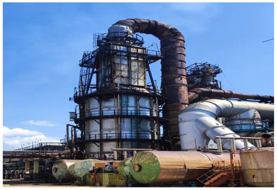
Figure 1.
Image of the F-101 furnace at the “Hermanos Díaz” refinery in Santiago de Cuba, Cuba.
Considering the importance and relevance of increasing the energy efficiency of the F-101 furnace, an analysis is made of the main variables involved in the heating process, highlighting the following:
- -
- The concentration of the process at the kiln inlet (k), the kiln outlet, or combined xi, yi, (moles/m3);
- -
- Product flow rate at the kiln inlet Qp, (m3/h);
- -
- Equilibrium outlet temperature Ts, (°C);
- -
- Fuel flow and calorific value Qc (m3/h), and qc (kcal/h);
- -
- Combustion air temperature Ta, (°C).
- -
- The concentration of combustion gasses in CO, CO2, and O2 (moles/m3);
- -
- Fuel gas outlet temperature Teg, (°C).
It is known that the desalted crude oil, coming from the second heat exchange system, enters the F-101 furnace at a temperature of 225 °C and then enters the convection zone to recover heat. Then, two coils enter the radiation zone of the furnace and, according to the oil furnace’s internal structure, there are two flow paths, so it is considered a multivariable MIMO system of the order 2 × 2, with a different behavior from that of a conventional SISO furnace.
Figure 2 shows the process of heating the desalted crude oil in the furnace in two steps to 350 °C. This oil heating process is controlled by two cascade control loops that link the crude oil outlet temperature to the fuel oil flow to the burners.
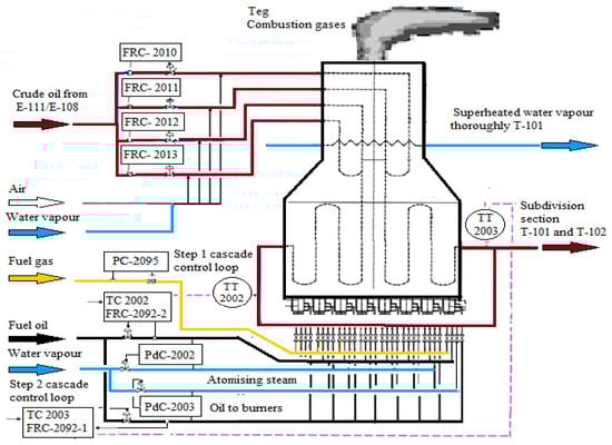
Figure 2.
General schematic of the F-101 furnace.
Figure 3 shows the structure of the cascade control scheme using the TC 2002 and FC 2092-1 controllers for step 1 and the TC 2003 and FC 2092-2 controllers for step 2. In addition, other variables of interest, such as crude oil load, liquid fuel oil consumption, fuel gas pressure, and stack gas temperature, are controlled.
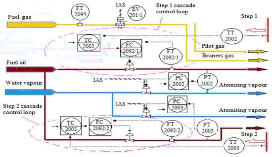
Figure 3.
Control structures existing at each step.
2.2. Dynamic Furnace Model
Furnace modeling aims to analyze and/or predict the system’s behavior using differential equations. Depending on the process’s nature and the available knowledge, many different models can be built to represent it [20]. According to literature reports [21,22], oil heating furnaces behave as first-order systems with transport delay or employ other system identification methods, such as ARMAX and BJ, as polynomial systems.
Considering the importance of the F-101 furnace in the atmospheric distillation stage, from the energetic and economic points of view, it was proposed to determine the mathematical model that represents the operating conditions and the behavior of the furnace under perturbations that guarantee the evaluation of energy efficiency [23].
For the study of this furnace, an experimental identification process was required to obtain dynamic models that accurately characterize the furnace’s behavior, so a set of sensors that measure the fundamental variables was installed. In addition, furnaces have complex dynamics, and linear approximations can be used to model them. Another consideration in our study is that identifying the response to a step signal at the furnace inlet can be used, which relates the variation in the input fuel for the burners to the variation in the crude oil temperature at the outlet. Finally, we considered that the furnace model will be represented generically as a first-order transfer function with delay and as a transfer function in the form of polynomials using the ARX, ARMAX, and BJ structures. The 1st-order model with transport delay is described in Equation (1).
where k is the gain of the first-order system, T is the time constant of the first-order system, and Td is the transport delay time constant. The ARX-, ARMAX-, and BJ-type models are parametric and include polynomial terms. They can be fitted to the experimental data by least squares estimation methods.
The ARX-type model has the form:
The ARMAX-type model has the form:
The BJ-type model has the form:
where y(t) is the output; u(t) is the input; e(t) is the white noise; q is the shift operator; nk is the delay; and B(q), F(q), C(q), and D(q) are polynomials in q.
The experiment was designed taking into consideration the installed PCS 7 distributed control system (DCS). The variables involved in the crude oil heating process in the F-101 furnace are measured and controlled through the DCS. The DCS is composed of sensors, transmitters, transmission buses, programmable controllers, and control valves (Figure 2 and Figure 3). High-precision instruments for the measurement and control of temperature, pressure, and flow are installed. This instrumentation is used in the F101 furnace’s experimental identification process.
The fuel oil flow data to the burners Qfq1(t), Qfq2(t) and the crude oil outlet temperatures Ts1(t) and Ts2(t) were obtained from the plant database, which records the variables and signals from the F-101 furnace. Several experiments were conducted. Each experiment consisted of varying instantaneously (unitary step) the fuel flow of each inlet and keeping the other inlet unchanged. For each experiment, the output temperature of each furnace step was measured. The sampling time for each experiment was 10 s.
The furnace’s fundamental parameters were maintained in a controlled environment, when the fuel flow was disturbed in each of the steps independently, obtaining thermal profiles that served as a basis for the experimental identification of the process.
In the process of the furnace’s experimental identification, it is considered a black box system with input and output signals to perform a set of experimental runs that will provide the necessary information on the inputs and outputs during the behavior of the furnace to its steady state. With this dynamic input-output relationship we obtain the mathematical model. Therefore, it is necessary to perform an analysis of the main variables involved in the process.
The measurements were obtained at the exit of each of the process steps, Ts1 and Ts2 (feedstock temperatures), by perturbing the input of a furnace step with a known step (the flow of fuel oil to the burners) and observing the behavior of the feedstock exit temperature in that step while keeping the other parameters constant in that step. In addition, the degree of influence of the different steps should be analyzed by recording the variables of interest shown in Table 1.

Table 1.
Variables analyzed in this study.
MATLAB R2018b was used to determine the model parameters, which provides a programming and simulation environment for handling data, functions, and graphics, as well as a set of specialized libraries for different application areas, such as the System Identification toolbox, which facilitates the estimation of dynamic system models from experimental data.
The experimental identification method used is based on the reaction curve that shows a response with an increasing asymptotic behavior, whose model does not take into account some parameters such as the alignment and the effects of the burner flame height and the variations in the composition of the fuel gas and the steam quality, which influence the atomization of the fuel oil. However, these undesirable effects were minimized in the multivariable model obtained by maintaining strict control over these effects.
The resulting experiment behaviors correspond to the generic transfer function given in Equation (1) and are shown in Figure 4 and Figure 5.
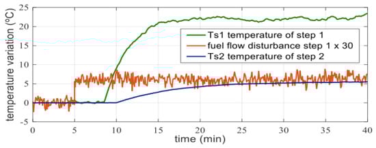
Figure 4.
Experimental furnace behavior when step 1 is perturbed with a variation in fuel flow.
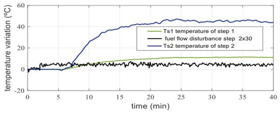
Figure 5.
Experimental furnace behavior when step 2 is perturbed with a variation in fuel flow.
Measurements of the variables of interest were employed to obtaining the model parameters given in Equation (1). The models with the best quality indicators (percentage of fit (%FIT)) were obtained using the Matlab identification toolbox. The multivariable modeling performed is shown in Table 2, with quality parameters evidenced in the calculated % FIT showing the adaptability and integration of the obtained models [17].
Table 2.
Parameters of the general multivariate model.
Taking into account that delays are not considered, the multivariable system of the furnace can be expressed as follows:
Obtaining the representation in state variables as shown below.
System equations:
where each state variable represents the variation in the corresponding variable :
- x1—temperature at step 1;
- x2—fuel oil flow in step 1;
- x3—fuel oil flow in step 2;
- x4—temperature at step 2.
Output equations:
Expressing the system in matrix form gives Equations (13) and (14),
2.3. Existing Control Strategy
With the model obtained and the PI control structures installed, the simulation was carried out, and the system’s behavior and the instabilities that it presents around the control target were observed to determine the system’s possibilities for minimizing them and obtaining a final product of higher quality while reducing energy consumption. The dynamic behavior shown in Figure 6 was obtained when the cascade regulators of the kiln steps were adjusted, and their inputs were subjected to step perturbations.
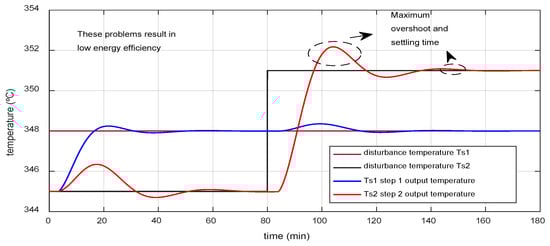
Figure 6.
Dynamic behavior of the temperature in the presence of steps in the inputs.
As can be seen, the furnace’s energetic behavior is limited when using the PI control structures, as reflected in the maximum overshoot and long settling times before the perturbations in the reference. To demonstrate the consistency of the existing control structure, the system was subjected to sinusoidal perturbations at the inputs, showing the dynamic behavior shown in Figure 7. As can be seen, monitoring the furnace temperatures in the face of disturbances is inaccurate, affecting its energy performance.
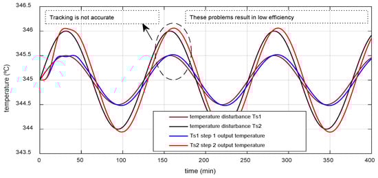
Figure 7.
Dynamic behavior of the temperature in the presence of sine waves at the inputs.
In modern control theory, one of the most critical problems that has been solved is related to the regulator, which consists of controlling a plant of a known order to follow reference signals and/or reject disturbances modeled by an external generator, called an exosystem; that is, the design of a control law to impose a steady-state response to the system that guarantees stability and bounded tracking errors [24,25,26].
2.4. The Design of the Linear Controller for the F101 Furnace
Since the control objective in the F101 furnace is to maintain the predetermined temperature of the crude oil at each step, the following exosystem is proposed.
Equation (15) describes an autonomous system defined in a neighborhood W of the origin of which models the class of reference signals taken into consideration—assumed to be a smooth vector field over W. The control action on the system represented by Equations (15) and (16) must be provided by a feedback controller, which processes the information received to ensure the desired control input. Characteristically, the structure of the controller will depend on the amount of information available for feedback, so it is common to find two types of controller structures:
- Full-information controller—if all components of the x states of the plant and all components of the W states of the exosystem are measurable.
- Error feedback controller—in which only the tracking error information is available.
Therefore, S and Q have the following form:
These expressions show that t and t.
The selection of this exosystem allows for the adjustment of constant reference signals (α = β = 0) and cosine signals of frequency α and β, which allows for the study of the performance of the closed-loop system at the simulation level. Following Linear Regulator Theory, a control law u will be designed as follows:
The problem of the linear regulator in the state feedback has a solution if and only if there exist matrices Γ and ∏ that solve Equations (20) and (21). Whereas, in the nonlinear case, the gain matrix k is selected such that the spectrum σ (A + B k) ∈ .
Therefore, it is necessary to find the matrices Γ and ∏ that give solutions to the following matrix equations:
Equations (20) and (21) are known as the Regulator equations or Francis equations [8], which have a solution ∏ and Γ for each Q, if and only if the rows of the matrix:
are linearly independent for all λ ∈ σ (S)
Calculating the values of the matrices Γ and ∏ for the coefficients of variation in the exosystem α = 0 and β = 0, corresponding to step excitations at the inputs, we obtain:
To determine the profit matrix k, we select the eigenvalues of the matrix A + Bk that all have negative real parts.
Using MATLAB, we obtained the result of placing the eigenvalues in R = [−1.0 −1.1 −1.2 −1.3].
Equation (19) and the calculated values of the matrices, Γ and k are used as a starting point for designing the system’s linear regulation control law. This control law will be given, in general, by Equations (26) and (27):
2.5. The Validation of the Model Using Criteria on “The Theory of Close Models”
The starting point is to apply the approach given in [27,28,29,30,31], on the perturbed systems to find a final value γ, which gives the measure of how far the nominal dynamics can move away from the model used in the design and still approximately meet the control objective when applied to the real plant.
Suppose the control obtained through the model can solve the control objective of the actual plant approximately, i.e., with minor bounded errors in fulfilling the purpose. In that case, it can be said that “the model obtained from the system is close to the plant”, thus fulfilling the objective of the output regulation.
If the above conditions are met, the model of the actual plant can be said to be “Validated” for the calculated linear regulation control law, which guarantees the fulfillment of the control objective foreseen for the system under analysis.
We start from the following aspirational model , where A is a known Hurwitz matrix and from the fact that .
As it is positive definite.
To find the last coordinate, the Lyapunov equation is solved by taking Q = I,
Resulting in the matrix P,
Then, the values of λmin(Q) = 1; λmax(P) = 71.0615 are determined to calculate the final coordinate of the system using Equation (30),
Therefore, γ < 0.007, i.e., the system converges to the solution variety whenever this convergence ratio is satisfied.
It can be concluded that the model obtained from Furnace F101 is “Validated” by applying the “Theory of Close Models” since it meets the plant’s requirements within certain limits. From all the previous analyses, it can be stated that the perturbed model of the plant has the following form:
where g(t,x) is a vector that contains the possible last values that tell how far the nominal dynamics can be moved away and whether the control objective is met. This vector has the form:
If the vector g(t,x) is substituted into expression (32), the perturbed model of the plant is obtained:
3. Results and Discussion
3.1. Linear Adjustment in the Furnace
With the obtained model of the multivariable plant, and after considering the disturbance term as zero (nominal dynamics), the designed control law, and the benefits of the MATLAB software package (R220a version), the system’s behavior will be obtained under different types of excitations in the input signals.
Figure 8 shows the dynamic behavior of the nominal model of the system when its inputs are excited with step signals. It shows the increase in the system’s response speed and the decoupling effect between the variations in the signals at the inputs. This behavior measures the quality of the response obtained so that the system quickly converges to its asymptotically stable equilibrium points.
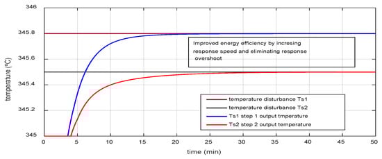
Figure 8.
Dynamic temperature behavior in the presence of steps in the inputs.
Figure 9 shows the dynamic behavior of the nominal model of the system when its inputs are excited with sinusoidal reference signals of the form T1ref. = 0.8 sin 0.5t and T2ref. = 0.5 sin t. It is observed that the system’s tracking of these reference signals is accurate, so it can be asserted that the solution variety of the system is effective [7].
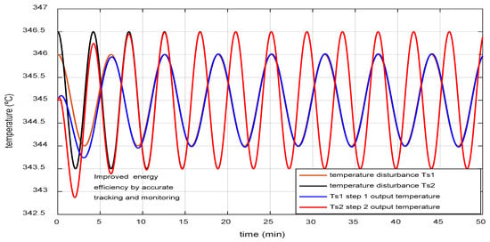
Figure 9.
Dynamic temperature behavior in response to sine wave signals at the inputs.
The linear controller achieves decoupling between variables by ensuring control of a plant of a known order to track reference signals and/or rejecting disturbances modeled by an external generator by imposing the fact that the system has a steady-state response with stability and bounded tracking errors.
The linear regulator is adjusted by varying the different components of the gain matrix k. This makes it possible to apply the results of the design of a linear regulator for a given model to the real system, making minor adjustments to improve its performance, thus compensating for possible uncertainties.
The system’s behavior when its states are perturbed shows that it can guarantee the fulfillment of the control objectives, demonstrating its ability to converge to its equilibrium points in an asymptotically stable manner.
The robustness of the linear regulation control strategy ensures a level of invariance in the performance of the temperature control system (short-, medium-, and long-term stability, at least) in the face of uncertainty in the furnace model [18].
The linear regulation control strategies apply to some industrial installations, specifically furnaces, and heaters, which could report considerable savings. The linear control adapts to different operating conditions, which contributes to the improvement of operating conditions by reducing process instabilities and the associated losses and ensuring the monitoring of reference signals.
Likewise, when the temperature control system works in a stable environment, it guarantees an adequate thermal profile inside the furnace, reducing and/or eliminating the hot spots that cause failures. The process’s stable operation results in an increase in operational reliability and minimizes maintenance costs.
3.2. Energy and Environmental Assessment of the Furnace
Next, we will discuss how the F-101 furnace’s energy and environmental indicators behaved under the different control strategies. Considering their importance from an energy and environmental point of view, the system analyzed the following indicators: fuel oil flow, energy efficiency, combustion flue gas temperature, and CO2 emissions to the atmosphere.
To calculate the furnace’s efficiency (), the valuable heat absorbed by crude oil in the heating process and the heat provided by the combustion of liquid fuel oil and fuel gas are determined, and their relationship is expressed in Equation (34).
where Qc is the proper heat absorbed by the crude oil (kcal/h), Qf is the heat given up by the combustion of the fuel oil (kcal/h), and Qg is the heat given up by the combustion of the fuel gas (kcal/h).
Equation (35) determines the CO2 emissions to the atmosphere due to the combustion of the liquid fuel oil.
where Fc is the fuel oil flow (m3/h), ρf is the density of the fuel oil (kg/m3), and 75.5 is the emission factor for industrial furnaces, which is expressed in kg CO2/TJ, representing the kg CO2 emitted to the atmosphere per ton of fuel burned in the furnace (kg/ton). In addition, Fc is the fuel oil flow to the burners (m3/h), and Tgc is the flue gas temperature (°C). These last parameters were obtained from the measurements made in the existing distributed control system.
Table 3 shows the results obtained from the behavior of some energy indicators of the furnace when the PI control strategy was applied. The values of these energy indicators were established during the whole month of August 2024, taking 10 samples at different moments of the operation of the plant, taking into account the stability of essential parameters of the process, such as the crude oil load to the unit, the stability of the burner flame, the correct atomization and temperature of the fuel oil in the burners, the opacity of the gasses, the temperature of the combustion gasses, and the consistency of the data of these experiments.
Table 3.
Furnace performance indicators with the PI control scheme.
As can be seen, the efficiency value of 69% is lower than the furnace’s design value. Therefore, due to its limitations, it is proposed to modify the control of the liquid fuel loop to the furnace to increase efficiency and reduce fuel consumption and CO2 emissions to the atmosphere.
Table 4 shows the values of the energy indicators’ behavior after the implementation of the linear regulation control structure at the same instant that the samples were taken with the PI control strategy.
Table 4.
Performance indicators of the furnace with the linear regulation scheme.
A comparative analysis of the two control strategies applied to the furnace showed that with the implementation of the linear regulation law in the furnace’s liquid fuel control loop, there is a fuel oil saving of 5% (0.74 m3/day). This saving has repercussions in terms of the reduction in the operating costs of the plant and of the gaseous pollutant load to the atmosphere, referred to as CO2, of between 3 and 5%, which is reflected in the decrease in the temperature of the combustion gasses at exit of the chimney by 2%, achieving an increase in efficiency of 1.5%.
Figure 10 shows a comparative analysis of the efficiency and CO2 emissions of the F-101 furnace when the existing PI control strategy was applied to the RL linear control strategy. The results show improvements in the kiln indicators when the control strategy with linear regulation is used, which increases energy efficiency and decreases environmental pollutants.
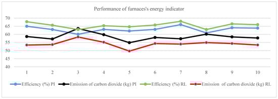
Figure 10.
The behavior of the furnace’s energy indicators under different control strategies.
4. Conclusions
This study shows the results achieved to improve the energy efficiency of the F-101 crude oil heating furnace by designing a linear control law. The variables used in the furnace model enabled the evaluation of the existing control law by studying the system’s behavior through simulations, showing the limitations of this control strategy.
The analysis of the output regulation problem in a linear plant with a disturbance term makes it possible to assert that the design of a state feedback control law, based only on the nominal model of the plant, guarantees the monitoring of the reference signals. In addition, the linear control law allows for the natural involvement of the main variables of the process and its disturbances as a multivariable system, guaranteeing the fulfillment of the control objective.
When comparing the results obtained with the use of the linear regulator designed concerning other conventional control strategies, it is evident that overruns decreased by 6%, the system response speed increased by more than 5 min, and the fuel consumption decreased by 5%, which is equivalent to 0.74 m3/day of fuel oil that is no longer used. All these indicators result in the improved energy performance of the F-101 furnace.
The use of linear regulation techniques in this furnace contributes to improving the energy efficiency by 1.5%, ensuring an improvement in the combustion of the technological installation by decreasing the temperature of the furnace exhaust gasses by 5–8 °C. An environmental impact is also obtained by reducing CO2 pollution by 3–5%.
Author Contributions
Conceptualization, F.J.-P., L.P.-P., M.R.F.-B. and E.E.S.-L.; methodology, L.P.-P., E.E.S.-L. and J.R.N.-A.; software, F.J.-P., E.E.S.-L. and J.R.N.-A.; validation, L.P.-P., F.J.-P., M.R.F.-B. and J.R.N.-A.; formal analysis, F.J.-P., M.R.F.-B. and L.P.-P.; investigation, F.J.-P., L.P.-P., M.R.F.-B. and E.E.S.-L.; resources, J.R.N.-A.; data curation, F.J.-P., L.P.-P. and M.R.F.-B.; writing—original draft preparation, J.R.N.-A., L.P.-P. and M.R.F.-B.; writing—review and editing, L.P.-P., J.A.T.-G. and J.R.N.-A.; visualization, J.R.N.-A. and J.A.T.-G.; supervision, L.P.-P. and E.E.S.-L.; project administration, F.J.-P., L.P.-P. and E.E.S.-L.; funding acquisition, F.J.-P., L.P.-P., J.A.T.-G. and J.R.N.-A. All authors have read and agreed to the published version of the manuscript.
Funding
This research received no external funding.
Data Availability Statement
Data are contained within the article.
Conflicts of Interest
The authors declare no conflicts of interest.
References
- Lobelles Sardiñas, G.O.; Morejón Gil, R.; García Conde, L.E.; Font Prieur, D.Y. Technological improvement in the F-203 furnace of Refinería Cienfuegos S.A to increase its energy efficiency. Ing. Energetica 2021, 42, e2008. [Google Scholar]
- Mullinger, P.; Jenkins, B. Industrial and Process Furnaces: Principles, Design and Operation, 2nd ed.; Butterworth-Heinemann: Oxford, UK, 2014; pp. 1–639. [Google Scholar] [CrossRef]
- Worrell, E.; Galitsky, C. Energy Efficiency Improvement and Cost Saving Opportunities for Petroleum Refineries. An ENERGY STAR Guide for Energy and Plant Managers. 2005. Available online: https://www.osti.gov/servlets/purl/862119 (accessed on 17 January 2025).
- Materán, S.M. Energy efficiency in oil refineries: A look at the efforts and actions taken by the refining industry at the international and regional level. EnerLAC Rev. Energía Latinoam. Caribe 2018, 2, 72–105. Available online: https://enerlac.olade.org/index.php/ENERLAC/article/view/49 (accessed on 17 January 2025).
- Rivas-Perez, R.; Feliu-Batlle, V.; Castillo-Garcia, F.J.; Benitez-Gonzalez, I. Temperature control of a crude oil preheating furnace using a modified Smith predictor improved with a disturbance rejection term. IFAC Proc. Vol. 2014, 47, 5760–5765. [Google Scholar] [CrossRef]
- Feliu-Batlle, V.; Rivas-Perez, R. Control of the temperature in a petroleum refinery heating furnace based on a robust modified Smith predictor. ISA Trans. 2021, 112, 251–270. [Google Scholar] [CrossRef]
- Isidori, A.; Byrnes, C.I. Output regulation of nonlinear systems. IEEE Trans. Autom. Control 1990, 35, 131–140. [Google Scholar] [CrossRef]
- Francis, B.A. The linear multivariable regulator problem. In Proceedings of the 1976 IEEE Conference on Decision and Control including the 15th Symposium on Adaptive Processes, Clearwater, FL, USA, 1–3 December 1976; pp. 873–878. [Google Scholar] [CrossRef]
- Hu, Y.; Tan, C.; Broughton, J.; Roach, P.A.; Varga, L. Nonlinear dynamic simulation and control of large-scale reheating furnace operations using a zone method based model. Appl. Therm. Eng. 2018, 135, 41–53. [Google Scholar] [CrossRef]
- Aguilar Malavé, J.S. Control Predictivo Basado en Modelo Para un Sistema Tipo SISO de Nivel de Líquido Representado en Variables de Estados y su Comparación con el Control PID y Control por redes Neuronales Artificiales. La Libertad, Universidad Estatal Península de Santa Elena (UPSE), School of Systems and Telecommunications. 2023. Available online: https://repositorio.upse.edu.ec/handle/46000/9608 (accessed on 17 January 2025).
- Li, G.; Ji, W.; Wei, L.; Yi, Z. A novel fuel supplies scheme based on the retrieval solutions of the decoupled zone method for reheating furnace. Int. Commun. Heat Mass Transf. 2023, 141, 106572. [Google Scholar] [CrossRef]
- Espin, J.; Castrillon, F.; Leiva, H.; Camacho, O. A modified Smith predictor based–Sliding mode control approach for integrating processes with dead time. Alex. Eng. J. 2022, 61, 10119–10137. [Google Scholar] [CrossRef]
- Raja, G.L.; Ali, A. Enhanced tuning of Smith predictor-based series cascaded control structure for integrating processes. ISA Trans. 2021, 114, 191–205. [Google Scholar] [CrossRef]
- Mejía, C.; Camacho, O.; Chavez, D.; Herrera, M. A modified smith predictor for processes with variable delay. In Proceedings of the 2019 IEEE 4th Colombian Conference on Automatic Control (CCAC), Medellin, Colombia, 15–18 October 2019; pp. 1–6. [Google Scholar] [CrossRef]
- Haratian, M.; Amidpour, M.; Hamidi, A. Modeling and optimization of process fired heaters. Appl. Therm. Eng. 2019, 157, 113722. [Google Scholar] [CrossRef]
- Gómez, A.; Correa, R. Implementation of a multivariable predictive control system in a fired heater. Dyna 2009, 76, 195–203. Available online: https://www.redalyc.org/articulo.oa?id=49611942019 (accessed on 17 January 2025).
- Jacas, P.F.; Peña, P.L.; Forgas, B.M.R. Experimental identification of a tubular preheating furnace for future control strategy analysis. In Proceedings of the III International Conference on Sustainable Energy Development, Villa Clara, Cuba, 13–17 November 2023. [Google Scholar]
- Zhang, R.; Cao, Z.; Li, P.; Gao, F. Design and implementation of an improved linear quadratic regulation control for oxygen content in a coke furnace. IET Control. Theory Appl. 2014, 8, 1303–1311. [Google Scholar] [CrossRef]
- Abreu, N.E.C. Adjustment of Controllers in the Fuel Control Loops in the Furnaces of the Cienfuegos S.A; Refinery; Automatic Control Department, Universidad Marta Abreu de Las Villas: Villa Clara, Cuba, 2021; Available online: https://dspace.uclv.edu.cu/handle/123456789/13217 (accessed on 17 January 2025).
- Liu, J.; Guo, N.; Peng, Y.; Li, W.; Qiao, J.; Gao, X.; Xiong, W. Adaptive sliding mode control of petrochemical flare combustion process based on radial basis function network. Chin. J. Chem. Eng. 2024, 76, 318–326. [Google Scholar] [CrossRef]
- Singh, S.; Kumar, K.; Patwardhan, S.C. Development of Block Oriented Recursive and Constrained Parameter Estimation Schemes for ARMAX Models. IFAC-PapersOnLine 2022, 55, 7–12. [Google Scholar] [CrossRef]
- Schulz, E.; Janda, O.; Schultalbers, M. On LPV System Identification Algorithms for Input-Output Model Structures and their Relation to LTI System Identification. IFAC-PapersOnLine 2018, 51, 1098–1103. [Google Scholar] [CrossRef]
- Chunsheng, W.; Yan, Z.; Zejun, L.; Fuxiang, Y. Heat transfer simulation and thermal efficiency analysis of new vertical heating furnace. Case Stud. Therm. Eng. 2019, 13, 100414. [Google Scholar] [CrossRef]
- Isermann, R. Advanced methods of process computer control for industrial processes. Comput. Ind. 1981, 2, 59–72. [Google Scholar] [CrossRef]
- Güray, S. A Review of quadrotor UAV: Control and SLAM methodologies ranging from conventional to innovative approaches. Robot. Auton. Syst. 2023, 161, 104342. [Google Scholar] [CrossRef]
- Peña-Pupo, L.; Martinez-Garcia, H.; García-Vílchez, E.; Fariñas-Wong, E.Y.; Núñez-Álvarez, J.R. Combined Method of Flow-Reduced Dump Load for Frequency Control of an Autonomous Micro-Hydropower in AC Microgrids. Energies 2021, 14, 8059. [Google Scholar] [CrossRef]
- DeHaan, S.; Yang, C.H. Advanced Process Control System Design for a Refinery: A Case Study. IFAC Proc. Vol. 1986, 19, 81–89. [Google Scholar] [CrossRef]
- Hassan, K. Nonlinear Systems, 3rd ed.; Pearson Education: Upper Saddle River, NJ, USA, 1996; pp. 1–560. [Google Scholar]
- Shitong, W.; Zhaojing, W.; Zheng-Guang, W. The regulation controller design for linear random systems with an uncertain exosystem. Syst. Control Lett. 2022, 161, 105150. [Google Scholar] [CrossRef]
- Riaño Jaimes, C.; Diaz Rodríguez, J.; Mejía Bugallo, D. On-line method for optimal tuning of PID controllers using standard OPC interface. Inge CuC 2022, 18, 13–26. [Google Scholar] [CrossRef]
- Ricardo, A.R.; Benítez, I.F.; González, G.; Nuñez, J.R. Multi-agent system for steel manufacturing process. Int. J. Electr. Comput. Eng. 2022, 12, 2441. [Google Scholar] [CrossRef]
Disclaimer/Publisher’s Note: The statements, opinions and data contained in all publications are solely those of the individual author(s) and contributor(s) and not of MDPI and/or the editor(s). MDPI and/or the editor(s) disclaim responsibility for any injury to people or property resulting from any ideas, methods, instructions or products referred to in the content. |
© 2025 by the authors. Licensee MDPI, Basel, Switzerland. This article is an open access article distributed under the terms and conditions of the Creative Commons Attribution (CC BY) license (https://creativecommons.org/licenses/by/4.0/).