Abstract
This study introduces a novel, low-cost, non-contact measurement system for heat flux estimation based on an enhanced thermometric method. The customized system was designed and assembled to implement a non-contact, indirect approach for heat flux assessment. Developed as an affordable alternative to conventional contact-based techniques, it is suitable for historical buildings, where invasive sensors could compromise structural integrity. The system integrates real-time data acquisition, remote access via a web-based interface, and automated data processing, enhancing both usability and efficiency. Laboratory tests were conducted to evaluate its performance, with results compared against data from widely used heat flow plates and air/surface temperature sensors. The results showed good agreement between the proposed method and the reference data. Small differences were observed between the values measured by the air temperature sensors (0.10 °C on average), as well as by the contact and non-contact surface temperature sensors (0.12 °C on average). Finally, percentage variations between −6% and −5% in terms of heat fluxes confirmed the reliability of the non-contact approach. These findings provide a strong foundation for further testing, including applications in real buildings.
1. Introduction
Existing buildings are responsible for significant global energy consumption and associated greenhouse gas emissions [1,2,3,4]. Reliable and non-destructive techniques for characterizing the thermal performance of building envelopes are essential to facilitate and promote cost-effective mitigation solutions to fight climate change [5,6,7,8,9]. These interventions are relevant for high-density urban environments that include older, energy-inefficient building stock [9,10,11,12]. Further challenges arise when dealing with structures of architectural value, where measurement techniques involving contact sensors may be inappropriate [13]. In these cases, tailored strategies are required to assess the thermal performance of existing walls without compromising their integrity [14,15].
Starting from this, Italy represents a relevant case study, with a building heritage of which 60% is made up of buildings constructed before the entry into force of the 1976 energy efficiency regulations [16,17]. These older buildings exhibit less than optimal energy performance, contributing substantially to overall energy consumption and greenhouse gas emissions. In this context, accurate techniques for thermally characterizing building components are essential to identify structures requiring energy retrofits [18,19,20,21]. These approaches aim to minimize errors in the assessment of the performance of passive building components, preventing inappropriate and costly energy efficiency interventions and promoting cost-effective mitigation strategies for energy savings.
Thermal characterization of walls through experimental approaches poses considerable challenges due to changing environmental conditions, material degradation, and limited comprehensive data [22,23,24]. Various non-destructive experimental approaches for evaluating the thermal properties of building walls have been developed to address these issues, employing diverse measurement instruments and sensors [25].
Several non-destructive, contact-based approaches have been developed for evaluating the thermal performance of building walls [26]. The standardized heat flow meter (HFM) method entails directly installing a heat flux sensor on the inner wall surface and air temperature sensors [27,28,29]. This allows assessing the thermal transmittance through direct measurements of the heat flux crossing the wall and the measured temperature values.
Another reliable contact-based approach is the simple hot-box heat flow meter (SHB-HFM) method [30], which requires designing and constructing a small handmade hot box setup. This technique ensures a controlled thermal environment by enclosing the wall specimen between two chambers and quantifying the heat flux crossing the investigated wall. Its implementation can be challenging due to the complexity of installation and the high costs associated with the measurement system.
Additionally, the thermometric method (THM) is a well-established contact-based approach that relies on installing surface and air temperature sensors [31]. This technique, which is the least explored in the literature, indirectly computes the wall’s heat flux using only temperature measurements and the selected internal heat transfer coefficient [32].
Implementing the previously mentioned contact-based approaches to existing buildings, particularly historical structures, can be problematic. Installing sensors on the walls may result in undesirable damage or alteration of the building fabric due to the use of adhesive tape or paste.
Contactless techniques, such as quantitative infrared thermography (QIRT) [33,34,35,36,37,38], which utilizes infrared thermal imaging cameras, have emerged as promising alternatives to address the limitations of traditional sensor-based approaches for evaluating the thermal performance of building walls [39]. However, the accuracy and reliability of this non-contact technique are subject to ongoing investigation and debate, as specific environmental conditions are required to obtain reliable results. Another limitation of infrared thermography is the high costs associated with infrared thermal imaging cameras.
The overall cost of the instrumentation required for the use of the above-mentioned techniques has been analyzed by Evangelisti et al. [40]. The authors noted that costs can range from approximately €1700.00 (THM) up to over €30,000.00 (QIRT).
Based on this, a new low-cost customized measurement system for an enhanced thermometric method was designed and assembled for the application of a non-contact indirect approach for heat flux estimate. The system integrates an infrared thermometer for non-contact measurement, allowing tests without physical contact. This allows the thermal performance of historic building façades to be assessed where traditional methods might prove impractical. By providing an affordable and non-invasive alternative to conventional heat flux measurement techniques, this system addresses an important need in the field of building energy assessment, especially for historic or specially protected buildings. Different tests were conducted under laboratory conditions to understand the reliability of the proposed new system. The realization of a new low-cost customized measurement system can have relevant impacts: (i) the scientific impact is strictly related to the proposal of a new measuring system, characterized by innovative real-time data management, which represents an enhanced version of the thermometric method (the new experimental system will be able to acquire data without using sensors to be installed on the surfaces of the walls, thus reducing the issues currently shown by other techniques and preventing damages); (ii) the technical impact is represented by the step forward in the field of non-destructive techniques, proposing a new solution (moreover, constructing a low-cost system would provide access for researchers with limited budgets to carry out investigations in buildings); (iii) the economic impact is represented by the design of a moderately priced measuring system, which can be used in buildings of historical and architectural value.
2. Materials and Methods
The development of this new measurement system is the main objective of a research project entitled “THErmometric Method Enhancement for building wall THErmal Resistance evaluation” (THE-METHER). Within the project, the first prototype of the new measurement system has been designed and assembled, and the first laboratory tests have been conducted.
2.1. THE-METHER
This sub-section provides the details about the device, called THE-METHER, used in the experimental setup. THE-METHER, designed and developed as part of the namesake project, is a modular device consisting of four main hardware components: (i) a Raspberry Pi which is a single-board computer (SBC) serving as the core computational unit, (ii) a custom-designed hardware attached on top (HAT) that facilitates integration with multiple sensors, (iii) a set of sensors selected to fit the enhanced thermometric method (E-THM), and (iv) an external touch display that allows users to manage the device without needing a PC. The hardware setup is complemented by dedicated software to handle data acquisition and device management.
Regarding the Raspberry Pi, version 4, with 4GB of memory, was successfully tested. The HAT, designed explicitly for THE-METHER, acts as an interface between the Raspberry Pi and the sensors by exposing GPIO (general-purpose input/output) pins, enabling proper power delivery, supporting standard sensors communication protocols, e.g., I2C (Inter-Integrated Circuit) and W1 (One-Wire).
As for the sensors that can be integrated into THE-METHER, the system includes a low-cost hot-wire anemometer mounted on a PCB, i.e., the Wind Sensor Rev. P, powered by a dedicated 9V step-up circuit integrated into the HAT, and this anemometer is used to assess the airflow regime. Additionally, two DS18B20 temperature probes provide air temperature measurements, enhancing the device’s capability to monitor thermal conditions. The probes can measure temperatures from −55 °C to 125 °C, with an accuracy over the range of −10 °C to 85 °C equal to ±0.5 °C.
An MLX90614 infrared thermometer, with a narrow 5-degree field of view (FOV), is included to facilitate non-contact surface temperature measurements, a feature proposed in conjunction with the E-THM and particularly useful in applications where direct sensor contact is impractical or undesirable. At room temperature, the surface temperature of the measured object can reach an accuracy of ±0.5 °C, and the temperature measurement range is from −70 °C to 380 °C.
The system also supports up to two DHT22 sensors, which measure both temperature (−40 °C to 80 °C temperature readings with ±0.5 °C accuracy) and humidity (0–100% humidity readings with 2–5% accuracy) and offers the capability to connect Bluetooth and Wi-Fi sensors, thereby contributing to a more comprehensive characterization of both indoor and outdoor environments.
From a software perspective, the rationale behind THE-METHER is to function as an independent measurement unit that can also act as an endpoint for data retrieval. At startup, if THE-METHER does not detect a known local network, it enables an access point, allowing users to connect via their devices (e.g., smartphone, tablet, or laptop) and access a web-based, platform-independent graphical interface.
To ensure a structured and efficient implementation, a REST API (an application program interface following the representational state transfer architectural paradigm) has been developed to enable centralized management of the measurement process. The web-based graphical interface queries this API, which provides essential functionalities such as initiating and terminating measurements and interfacing with the various sensors connected to THE-METHER. The API architecture establishes a clear separation between backend logic, responsible for hardware communication, and the graphical user interface (GUI), which facilitates user interaction. The system achieves a more structured architecture that enhances maintainability and scalability by encapsulating the complexities of direct sensor communication within the API.
The graphical interface for THE-METHER was developed using Python 3.13.1 and Flask 3.1.0, ensuring a modular and flexible system design. This API-based architecture offers several advantages, including improved scalability, as new sensors and functionalities can be integrated with minimal modifications to the existing codebase. It also enhances maintainability, allowing backend updates to be performed independently of changes to the user interface. Furthermore, the adoption of Flask enables web-based interaction, allowing users to monitor and control the device remotely. The costs incurred for the construction of the prototype are listed in Table 1, including producer and country. The total cost of the components is less than €365.00.

Table 1.
Prototype component average costs (prices may differ depending on the supplier).
2.2. Thermally Insulated Box and Heat Bed Control Unit
A square wooden specimen measuring 0.3 m × 0.3 m, with a thickness of 0.015 m, was enclosed within a thermally insulated box. The hand-made box was constructed by assembling 0.05 m thick XPS panels into a structure measuring 0.6 m in height and width, with a 0.1 m thickness. Wooden panels were glued to the XPS to enhance structural stability.
The heating mat used in [41] was here replaced by a square heat bed from Creality, a 3D printer manufacturer, as the heating element. This aluminum heat bed allows homogeneous and controlled heating from 0 °C to 130 °C, with 1 °C increments, regulated via a control unit. Figure 1 depicts the 3D view of the insulated box and its dimensions, already used in [41]. Figure 2 provides a comparison in terms of the homogeneous heating capacity of the sample, demonstrating the improvement made to the setup via the heat bed.
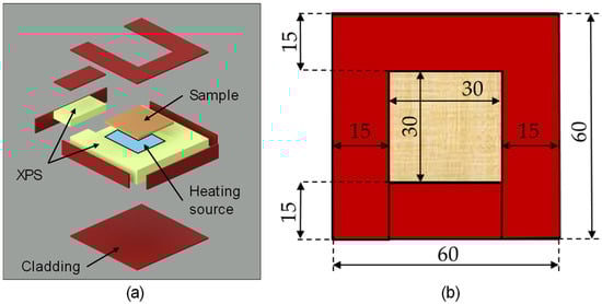
Figure 1.
3D view of the insulated box (a), and its dimensions in cm (b) (from [41]).
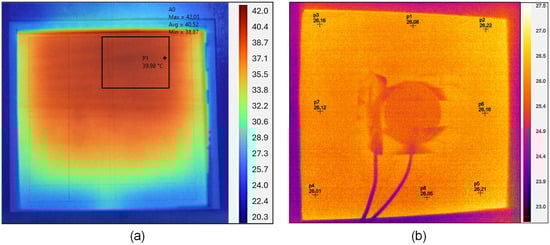
Figure 2.
Comparison in terms of homogenous heating of the sample: heating mat previously used (from [41]) (a); heat bed from Creality (b). The temperature scales are Celsius degrees.
2.3. Experimental Setup
Multiple sensors were installed to simultaneously measure and evaluate the thermal characteristics of the wooden sample, enabling a comparison of contact-based and non-contact approaches. The emissivity of the sample was identified in [41], where the reflector-based approach was applied, obtaining an emissivity of 0.84 for the sample. A widely used heat flux plate (Hukseflux, model HFP01 [42]) was installed to acquire data through a direct approach. A contact surface temperature sensor (LSI Lastem, model EST124 [43]) was positioned on the free-front surface of the wooden sample to compare the recorded data with those acquired by the MLX90614 infrared thermometer. An air temperature sensor (LSI Lastem, model EST033 [44]) was installed far from the heated sample to compare the logged data with those acquired by the DS18B20 temperature probes. The experimental setup is shown in Figure 3.
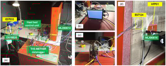
Figure 3.
The experimental setup: overall view (a); the new datalogger (b,c); heat flux plate and surface and infrared surface temperature sensors (d). Yellow color is used for LSI and Hukseflux sensors; green color is used for the new measuring system.
Additionally, a hot-wire anemometer TESTO 06280152 [45] was used to verify the air velocity data acquired by the Wind Sensor Rev. P near the sample. The schematic top view of the experimental setup is shown in Figure 4.
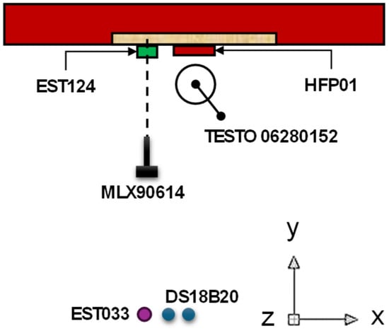
Figure 4.
Schematic top view of the experimental setup.
2.4. Methodological Approach
A preliminary evaluation was conducted to assess the surface thermal uniformity of the sample (as previously shown in Figure 2). The wood sample was heated until it reached a nearly constant temperature (steady state condition). The temperature of the heat bed was set to reproduce a temperature difference between the air and the surface of the sample similar to that occurring in real buildings. These conditions were reached by imposing a heat bed temperature equal to 30 °C, ensuring a temperature gradient approximately equal to 3 °C between the surface of the sample and the indoor air temperature.
The heat flux through the sample was evaluated using two approaches:
- (i)
- The direct, contact-based heat flow meter technique (HFM). The logged data was used as a reference.
- (ii)
- The contactless indirect enhanced thermometric method (E-THM) applied by means of the newly proposed customized measurement system. The tests were conducted with the infrared thermometer positioned at distances of 2.5 cm and 7 cm from the sample to evaluate the effect on the results.
The E-THM method relied on acquiring air velocity and indoor air temperature data from an anemometer and air temperature probes. Air velocity data can be useful for better identifying specific convective conditions. The anemometer position can be selected in accordance with the heat transfer theory, enabling the use of the free-stream velocity for applying the dimensionless groups theory for the heat transfer coefficients identification [46]. In this study, the anemometer was placed at a suitable distance from the heated sample, equal to 0.09 m.
The data collected, in terms of surface temperature (), indoor air temperature (), and air velocity (), were used to compute the dimensionless Grashof (Gr) and Reynolds (Re) numbers as follows:
where is the gravitational acceleration (equal to 9.81 m/s2), is the cubic thermal expansion coefficient of the fluid (equal to , where ), is the kinematic viscosity of the fluid, and is the vertical dimension of the heated sample.
As mentioned before, specific convective conditions can occur. Therefore, Gr and Re numbers can be used to compute the Richardson (Ri) number, to identify natural or forced convection conditions. Ri enabled the identification of the prevailing mode of convective heat transfer, which could be natural convection ( > 10), mixed convection (0.7 < < 10), or forced convection ( < 0.7). Once the convective heat transfer mode is identified, the Nusselt (Nu) number can be computed for the convective heat transfer coefficient assessment.
In almost all cases, natural convection conditions occur in buildings, for which the following equations can be applied to calculate Nu:
where Ra is the Rayleigh number, and Pr is the Prandtl number. Equation (5), established by Churchill and Chu [46], is suitable for most engineering applications, returning more accurate values compared to Equations (3) and (4).
Conversely, other equations can be utilized for forced convection conditions to determine Nu. Depending on the values of and Pr numbers, the flow regime can be identified as either laminar or turbulent. When the flow is in the laminar regime, with and , the following equation can be applied:
For the mixed convection scenario, it is possible to compute by employing the following formula:
It is well known that Nu is defined in function of the fluid thermal conductivity (λ), the geometric characteristic length (L), and the convective heat transfer coefficient (hc):
In this study, L represents the vertical dimension of the sample (equal to 0.3 m). The dimensionless numbers Gr, Re, and Nu depend on specific thermophysical properties. The film temperature (TFILM) was calculated within the range of 10 °C to 40 °C, which is typical for building physics applications. Based on TFILM, air thermal conductivity, kinematic viscosity (ν), thermal expansion coefficient (β), and the Prandtl number were determined. These properties were obtained through a linear regression approach using data from the Fluid Properties Calculator of the University of Waterloo [47].
Although thermophysical properties exhibit a nonlinear dependence on temperature, the selected temperature range allows for a linear regression approximation. This approach yields values that closely match those provided by the Fluid Properties Calculator, with exceptionally high R2 values (see Table 2). This approximation enabled the calculation of thermophysical properties for each acquisition time step with high accuracy.
Table 2.
Prandtl, kinematic viscosity, and thermal conductivity as a function of the film temperature (air).
When the temperature difference between two bodies is significantly smaller than their average temperature, the nonlinear relationship governing radiative heat transfer can be linearized. This allows for the determination of the radiative heat transfer coefficient (hr) using the following formula:
where ε is the sample emissivity, σ is the Stefan–Boltzmann constant, and Tavg is the average temperature of the surface and its surroundings. The total heat transfer coefficient (htot) is obtained by summing hc and hr. Using Newton’s law of cooling, heat fluxes can be calculated indirectly through the following equation:
The evaluation of measurement uncertainty was conducted in accordance with the ISO Guide to the Expression of Uncertainty in Measurement. In this study, only statistical uncertainty was considered. It was estimated through statistical analysis of repeated measurements, utilizing the standard deviation of the mean to quantify random variations. The combined standard uncertainty was then obtained by applying the uncertainty propagation law using the root sum of squares method [48,49]. To ensure consistency with international metrological standards, a coverage factor k = 2 was applied to estimate a 95% confidence interval.
3. Results and Discussion
3.1. Data Management and Web Interface
A web-based interface was developed for THE-METHER, enabling remote access via an IP address for measurement management, real-time data visualization, and data export. The interface includes a homepage, a measurement control panel for starting and stopping acquisitions, and configurable parameters such as acquisition timestep and file naming. A dedicated section allows users to monitor real-time data trends and download recorded measurements in CSV format for further analysis. This system enhances usability and accessibility, facilitating efficient data handling and visualization.
When an internet connection is available, THE-METHER can be accessed online, allowing remote interaction with the system. This feature enables flexible instrument management, facilitating remote operation, monitoring, and data retrieval without requiring direct physical access. Figure 5 shows three screenshots of the created web-based interface.
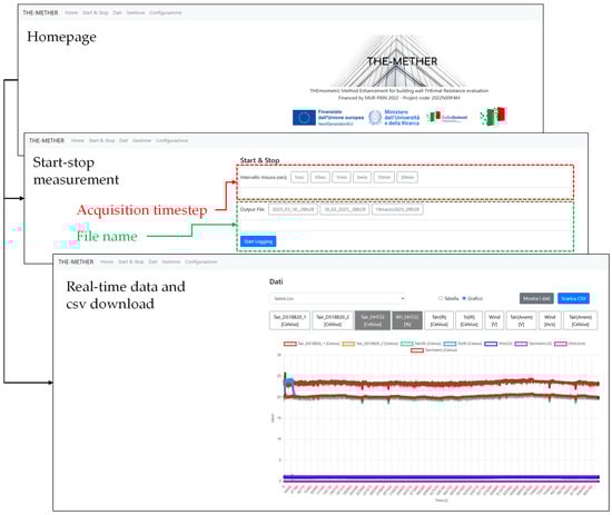
Figure 5.
Web interface created for data acquisition, visualization, and download.
3.2. HFM vs. E-THM
As mentioned before, the sample was heated through the heat bed until it reached a steady-state condition. Data were acquired every 10 s positioning the infrared thermometer in front of the sample, near the heat flux plate and the contact surface temperature. The first dataset was logged positioning the infrared thermometer at 2.5 cm. The air temperature sensors DS18B20 were sited near EST033. The results in terms of air and surface temperature data are shown in Figure 6a,b.
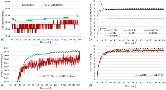
Figure 6.
Comparison between data obtained by installing the infrared sensor at 2.5 cm: air temperatures (a); surface temperatures (b); convective and radiative heat transfer coefficients (c); heat fluxes (d).
Examining the period of greatest thermal stability (approximately the last 50 min), it is possible to observe small differences between the sensors. Figure 6a shows Tair-avg (DS18B20) because the THE-METHER is equipped with two air temperature sensors, and the arithmetic mean of the values recorded by the probes was considered. It is possible to observe small differences between the values measured by the sensors, with values at most equal to about 0.10 °C. This agreement strengthens the robustness of the measurement system in monitoring environmental conditions. While the sensors demonstrate high accuracy in controlled laboratory conditions, their performance needs to be further validated in real-world applications. The full implementation of the system aims to assess the thermal transmittance of actual building walls, which will require incorporating external air temperature measurements. Given the potential influence of environmental factors, future studies should evaluate the system’s reliability under diverse operational conditions to ensure its applicability in in situ assessments.
Considering the same time interval, comparing the surface temperatures measured through the contact and contactless probes, it is possible to state that the measured values differ on average by 0.12 °C (see Figure 6b). This is reflected in terms of the difference in surface-air temperature, with values slightly above 3 °C. Regarding surface temperature measurements, the observed mean deviation between contact and non-contact probes suggests a high level of agreement, supporting the validity of the proposed method. However, a more pronounced oscillatory pattern over time can be observed using the non-contact sensor. These fluctuations may be attributed to dynamic interactions between the heating system and the surrounding environment, as well as the inherent response characteristics of the sensors. While these variations remain within an acceptable range for laboratory conditions, their potential impact on long-term measurements in real-world applications should be further investigated, particularly when assessing thermal transmittance in actual buildings.
Air velocity values acquired through the Wind Sensor Rev. P differ significantly from those measured by the hot-wire anemometer TESTO 06280152, highlighting a weakness that will need to be addressed in the future. The Wind Sensor Rev. P is designed mainly for outdoor applications, showing weakness for indoor applications although the measured range is nominally 0 m/s to 67 m/s. For this reason, Re was calculated with the data acquired by the TESTO anemometer, which recorded an average air speed of 0.08 m/s (compared to approximately 9.00 m/s measured on average by the Wind Sensor Rev. P). According to this, Ri and Ra values were obtained (see Figure 7a). A Ri equal to 5 is related to mixed convection conditions. However, in this specific case study, the low air velocity (0.08 m/s) and modest temperature difference indicate that natural convection could be predominant. The air velocity is low, which significantly reduces the contribution of forced convection. At such low velocities, the influence of inertia forces on the boundary layer development is minimal, allowing buoyancy effects to play a leading role in driving fluid motion. Additionally, the small temperature difference between the sample and the ambient air is sufficient to generate buoyancy-driven flows, further enhancing the role of natural convection. The characteristic length (0.3 m) used in the calculation of the Richardson number affects its numerical value (see Figure 7b). While the calculated value remains within the mixed convection range, the physical impact of forced convection could be weaker than what the numerical value of Ri alone implies.
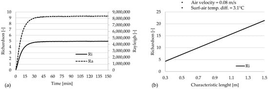
Figure 7.
Richardson and Rayleigh trends obtained from the measurement campaign (a); influence of the characteristic length on Ri considering specific boundary conditions (b).
Heat transfer coefficients obtained from contact sensors and THE-METHER probes showed highly similar values (see Figure 6c). The convective coefficients were obtained by applying Equation (5), suitable for most engineering applications and capable of returning more accurate values. For the convective component, hc was 2.57 W/m2K using LSI sensors and 2.55 W/m2K with THE-METHER. The radiative coefficient was 5.14 W/m2K with LSI sensors and 5.13 W/m2K with THE-METHER. Consequently, the total heat transfer coefficients were nearly identical: 7.71 W/m2K from LSI sensors and 7.68 W/m2K from THE-METHER.
What was previously stated regarding the potential condition of purely natural convection (despite a Ri equal to 5) can be proved by comparing the total heat transfer coefficients mentioned before, with those computed by making the ratio between the heat fluxes measured via HFM and the surface-air temperature differences obtained by the LSI instrumentation (named htot(HFM) in Figure 6c, and equal to 7.90 W/m2K on average).
According to these results, Figure 6d shows heat fluxes. The slightly oscillating heat flux pattern obtained by the HFM sensor is due to the frequent on–off switching of the heat bed to maintain a constant temperature. The results demonstrate a good agreement between the widely used direct method based on the heat flux plate and the indirect, non-contact approach implemented by the proposed new measurement system. The average values observed during the interval characterized by the greatest thermal stability were 25.33 W/m2 (HFM) and 24.10 W/m2 (E-THM), with an average percentage difference equal to −4.85%. This percentage variation is reduced by calculating Nu using Equation (3), according to the values of the Ra number, of the order of 106. The resulting percentage difference is −2.64%.
Table 3 summarizes the results and the related statistical uncertainties.
Table 3.
Values from the first test (infrared thermometer at 2.5 cm) with statistical uncertainties.
The second test was conducted with the infrared thermometer positioned 7 cm from the sample. The heat bed configuration remained identical to the previous test, maintaining a temperature of 30 °C. The acquired data exhibited similar trends, showing an initial increase followed by subsequent stabilization. For clarity and conciseness, the average values are presented in Table 4. Also, in this case, it is possible to observe quite similar air and surface temperature values, leading to similar heat transfer coefficients. Consequently, the average total heat transfer coefficients were similar when Equation (5) was applied: 7.70 W/m2K from LSI sensors and 7.67 W/m2K from THE-METHER. By comparing these total heat transfer coefficients with the average value deriving from the ratio between the heat fluxes measured via HFM and the surface-air temperature differences obtained by the LSI instrumentation (7.90 W/m2K), it is possible to observe almost negligible differences (lower than 3%).
Table 4.
Values from the second test (infrared thermometer at 7 cm) with statistical uncertainties.
Comparing the heat flux values obtained by E-THM and HFM shown in Table 4 allows us to identify a percentage variation equal to −5.85%. In this case as well, the percentage variation decreases when Nu is calculated using Equation (3), based on the Ra number, which is on the order of 106. The resulting variation is −3.66%.
The comparison between direct (HFM) and indirect (E-THM) heat flux measurements reveals relatively small differences, suggesting a high level of agreement between the two methods. The deviations can be attributed to several factors, including the influence of infrared sensor positioning, and slight variations in convective conditions. Additionally, the heat flux plate inherently alters the local thermal resistance at the measurement point, which may contribute to systematic discrepancies.
The statistical uncertainties shown in Table 3 and Table 4 highlight that the E-THM method presents a slightly higher variability compared to the direct HFM approach. This difference is expected, given that E-THM relies on multiple measurements. Uncertainties in individual sensor readings propagate through the calculations of heat transfer coefficients and heat flux following standard uncertainty propagation methods. This preliminarily suggests that the proposed method maintains competitive accuracy while eliminating the need for intrusive sensor installations.
In real buildings, natural convection is often the predominant heat transfer mechanism, particularly in those with radiator-based heating systems, which are widespread in Italy. Under these conditions, especially when wall heights exceed 2.5 m, the influence of mixed or forced convection is typically negligible.
Future in situ tests focusing on wall thermal transmittance will further assess the role of the anemometer, addressing its measurement limitations. Additional testing in buildings with different HVAC systems, using comparative instruments such as LSI and Hukseflux sensors, will help define the system’s operational boundaries, ensuring its reliability for in situ thermal transmittance assessments. THE-METHER is designed to operate across various HVAC configurations. Consequently, future developments will focus on integrating a more reliable anemometry system.
4. Conclusions
This study introduced THE-METHER, a novel, low-cost, contactless measurement system designed to estimate heat flux using an enhanced thermometric method. The system was tested under controlled laboratory conditions and compared with conventional sensors. The results demonstrated a high level of agreement between the proposed method and the reference data. Small differences between the values measured by the air temperature sensors, with values at most equal to about 0.10 °C, were observed. Furthermore, when comparing surface temperatures measured by contact and non-contact probes, the measured values showed differences of an average of 0.12 °C. Finally, percentage variations between −6% and −5% in terms of heat fluxes confirmed the reliability of the contactless approach.
A key strength of THE-METHER lies in its ability to provide real-time, remote data acquisition and processing via a web-based interface. This feature enhances accessibility, allowing users to manage, visualize, and download measurement data online. Additionally, the system minimizes invasive installation procedures, making it particularly suitable for applications involving historical buildings or sensitive surfaces where traditional contact sensors could cause damage.
Despite these advantages, a limitation was identified in the performance of the air velocity sensor, which exhibited significant discrepancies in air velocity measurements compared to a reference hot-wire anemometer. This issue affects the accuracy of convective heat transfer coefficient estimation and requires further investigation.
Future developments will focus on (i) integrating a more reliable anemometry system; (ii) designing a more definitive, enclosed system, while also assessing the feasibility of integrating advanced sensors; (iii) incorporating wireless air temperature sensors for in situ applications, enabling the evaluation of wall thermal transmittance in real buildings; and (iv) enhancing data management capabilities to implement convergence criteria, ensuring reliable thermal transmittance measurements in practical applications.
In addition, while the proposed measurement system demonstrated high reliability under controlled laboratory conditions (the E-THM method presents a slightly higher uncertainty, ±0.22 W/m2, compared to the direct HFM approach, ±0.04 W/m2), further research is required to refine uncertainty quantification. Moreover, the system behavior will need to be tested under different environmental conditions, under different ambient temperatures and humidity levels.
In conclusion, the proposed system represents a promising advancement in non-destructive thermal diagnostics, particularly for energy efficiency assessments in buildings. Further refinements will enhance its applicability in both research and field investigations.
Author Contributions
Conceptualization, L.E., T.d.R. and S.M.; methodology, L.E., E.D.C., S.M., C.G. and P.G.; software, S.M. and I.P.; validation, S.M., E.D.C. and I.P.; formal analysis, L.E. and E.D.C.; investigation, E.D.C. and S.M.; resources, L.E. and S.M.; data curation, C.G. and P.G.; writing—original draft preparation, L.E., S.M. and C.G.; writing—review and editing, T.d.R., D.A., C.G. and P.G.; supervision, L.E., T.d.R. and D.A.; project administration, L.E., D.A. and S.M.; funding acquisition, L.E. and D.A. All authors have read and agreed to the published version of the manuscript.
Funding
This research received the financial support under the National Recovery and Resilience Plan (NRRP), Mission 4, Component 2, Investment 1.1, Call for tender No. 104 published on 2 February 2022 by the Italian Ministry of University and Research (MUR), funded by the European Union—NextGenerationEU. Project Title: THErmometric Method Enhancement for building wall THErmal Resistance evaluation (Project code: 2022NX9F4M)—CUP F53D23001850006. Grant assignment Decree No. 961 adopted on 30 June 2023 by the Italian Ministry of Ministry of University and Research (MUR).
Data Availability Statement
Data will be made available upon request.
Conflicts of Interest
The authors declare no conflicts of interest.
Abbreviations
The following abbreviations are used in this manuscript:
| g | gravitational acceleration [m/s2] |
| hc | convective coefficient [W/m2K] |
| hr | radiative coefficient [W/m2K] |
| htot | total heat transfer coefficient [W/m2K] |
| k | coverage factor |
| L | characteristic length [m] |
| q | heat flux density [W/m2] |
| Tair int | air temperature [K, °C] |
| Tavg | average thermodynamic temperature [K] |
| Ts | surface temperature [K, °C] |
| wair | air velocity [m/s] |
| E-THM | enhanced thermometric |
| HFM | heat flow meter |
| Gr | Grashof [-] |
| Nu | Nusselt [-] |
| Pr | Prandtl [-] |
| Ra | Rayleigh [-] |
| Re | Reynolds [-] |
| Ri | Richardson [-] |
| β | cubic thermal expansion coefficient [1/K] |
| ε | emissivity [-] |
| σ | Stefan–Boltzmann constant [W/m2K4] |
| ν | kinematic viscosity [m/s2] |
References
- Li, Y.L.; Han, M.Y.; Liu, S.Y.; Chen, G.Q. Energy Consumption and Greenhouse Gas Emissions by Buildings: A Multi-Scale Perspective. Build. Environ. 2019, 151, 240–250. [Google Scholar] [CrossRef]
- Röck, M.; Saade, M.R.M.; Balouktsi, M.; Rasmussen, F.N.; Birgisdottir, H.; Frischknecht, R.; Habert, G.; Lützkendorf, T.; Passer, A. Embodied GHG Emissions of Buildings—The Hidden Challenge for Effective Climate Change Mitigation. Appl. Energy 2020, 258, 114107. [Google Scholar] [CrossRef]
- Pérez-Lombard, L.; Ortiz, J.; Pout, C. A Review on Buildings Energy Consumption Information. Energy Build. 2008, 40, 394–398. [Google Scholar] [CrossRef]
- Zhang, Y.; He, C.-Q.; Tang, B.-J.; Wei, Y.-M. China’s Energy Consumption in the Building Sector: A Life Cycle Approach. Energy Build. 2015, 94, 240–251. [Google Scholar] [CrossRef]
- Soares, N.; Martins, C.; Gonçalves, M.; Santos, P.; da Silva, L.S.; Costa, J.J. Laboratory and In-Situ Non-Destructive Methods to Evaluate the Thermal Transmittance and Behavior of Walls, Windows, and Construction Elements with Innovative Materials: A Review. Energy Build. 2019, 182, 88–110. [Google Scholar] [CrossRef]
- Alkhatib, H.; Lemarchand, P. Assessing Thermal Performance: An Experimental Study on U-Value Variability in Building Fabric Elements. Results Eng. 2025, 25, 103730. [Google Scholar] [CrossRef]
- Afaynou, I.; Faraji, H.; Choukairy, K.; Khallaki, K.; Akrour, D. Effectiveness of a PCM-Based Heat Sink with Partially Filled Metal Foam for Thermal Management of Electronics. Int. J. Heat. Mass. Transf. 2024, 235, 126196. [Google Scholar] [CrossRef]
- Al-Sallami, W.; Al-Damook, A.; Thompson, H.M. A Numerical Investigation of Thermal Airflows over Strip Fin Heat Sinks. Int. Commun. Heat Mass Transf. 2016, 75, 183–191. [Google Scholar] [CrossRef]
- Yang, Y.; Wu, T.V.; Sempey, A.; Dumoulin, J.; Batsale, J.-C. Short Time Non-Destructive Evaluation of Thermal Performances of Building Walls by Studying Transient Heat Transfer. Energy Build. 2019, 184, 141–151. [Google Scholar] [CrossRef]
- Kyritsi, E.; Katsaprakakis, D.; Dakanali, E.; Yiannnakoudakis, Y.; Zidianakis, G.; Michael, A.; Michopoulos, A. Energy Renovation of Two Historical Buildings in Mediterranean Area. J. Cult. Herit. 2025, 71, 106–113. [Google Scholar] [CrossRef]
- Defer, D.; Shen, J.; Lassue, S.; Duthoit, B. Non-Destructive Testing of a Building Wall by Studying Natural Thermal Signals. Energy Build. 2002, 34, 63–69. [Google Scholar] [CrossRef]
- Ruiz Valero, L.; Flores Sasso, V.; Prieto Vicioso, E. In Situ Assessment of Superficial Moisture Condition in Façades of Historic Building Using Non-Destructive Techniques. Case Stud. Constr. Mater. 2019, 10, e00228. [Google Scholar] [CrossRef]
- Akkurt, G.G.; Aste, N.; Borderon, J.; Buda, A.; Calzolari, M.; Chung, D.; Costanzo, V.; Del Pero, C.; Evola, G.; Huerto-Cardenas, H.E.; et al. Dynamic Thermal and Hygrometric Simulation of Historical Buildings: Critical Factors and Possible Solutions. Renew. Sustain. Energy Rev. 2020, 118, 109509. [Google Scholar] [CrossRef]
- Genova, E.; Fatta, G. The Thermal Performances of Historic Masonry: In-Situ Measurements of Thermal Conductance on Calcarenite Stone Walls in Palermo. Energy Build. 2018, 168, 363–373. [Google Scholar] [CrossRef]
- de Rubeis, T.; Tanfoni, A.; Ciccozzi, A.; Pasqualoni, G.; Paoletti, D.; Ambrosini, D. Exploring Alternative Experimental Approaches for Wall Heat Transfer Assessment—The Enhanced Thermometric Method. In Proceedings of the IEEE 2024 9th International Conference on Smart and Sustainable Technologies (SpliTech), Bol and Split, Croatia, 25–28 June 2024; pp. 1–5. [Google Scholar]
- Law 30 March 1976, n. 373—Rules for the Containment of Energy Consumption for Thermal Uses in Buildings. (GU General Series n.148 of 06-07-1976). Available online: https://www.gazzettaufficiale.it/eli/id/1976/06/07/076U0373/sg (accessed on 1 March 2025).
- Vettore, M.; Donà, M.; Carpanese, P.; Follador, V.; da Porto, F.; Valluzzi, M.R. A Multilevel Procedure at Urban Scale to Assess the Vulnerability and the Exposure of Residential Masonry Buildings: The Case Study of Pordenone, Northeast Italy. Heritage 2020, 3, 1433–1468. [Google Scholar] [CrossRef]
- Lambie, E.; Saelens, D. Identification of the Building Envelope Performance of a Residential Building: A Case Study. Energies 2020, 13, 2469. [Google Scholar] [CrossRef]
- Deconinck, A.-H.; Roels, S. Comparison of Characterisation Methods Determining the Thermal Resistance of Building Components from Onsite Measurements. Energy Build. 2016, 130, 309–320. [Google Scholar] [CrossRef]
- Sassine, E. A Practical Method for In-Situ Thermal Characterization of Walls. Case Stud. Therm. Eng. 2016, 8, 84–93. [Google Scholar] [CrossRef]
- Bienvenido-Huertas, D.; Pérez-Ordóñez, J.L.; Moyano, J.; Seara-Paz, S. Towards an In-Situ Evaluation Methodology of Thermal Resistance of Basement Walls in Buildings. Energy Build. 2020, 208, 109643. [Google Scholar] [CrossRef]
- Balaji, N.C.; Mani, M.; Venkatarama Reddy, B.V. Dynamic Thermal Performance of Conventional and Alternative Building Wall Envelopes. J. Build. Eng. 2019, 21, 373–395. [Google Scholar] [CrossRef]
- Teni, M.; Krstić, H.; Kosiński, P. Review and Comparison of Current Experimental Approaches for In-Situ Measurements of Building Walls Thermal Transmittance. Energy Build. 2019, 203, 109417. [Google Scholar] [CrossRef]
- Mobaraki, B.; Castilla Pascual, F.J.; García, A.M.; Mellado Mascaraque, M.Á.; Vázquez, B.F.; Alonso, C. Studying the Impacts of Test Condition and Nonoptimal Positioning of the Sensors on the Accuracy of the In-Situ U-Value Measurement. Heliyon 2023, 9, e17282. [Google Scholar] [CrossRef] [PubMed]
- Evola, G.; Lucchi, E. Thermal Performance of the Building Envelope: Original Methods and Advanced Solutions. Buildings 2024, 14, 2507. [Google Scholar] [CrossRef]
- Bienvenido-Huertas, D.; Moyano, J.; Marín, D.; Fresco-Contreras, R. Review of in Situ Methods for Assessing the Thermal Transmittance of Walls. Renew. Sustain. Energy Rev. 2019, 102, 356–371. [Google Scholar] [CrossRef]
- Gaspar, K.; Casals, M.; Gangolells, M. Review of Criteria for Determining HFM Minimum Test Duration. Energy Build. 2018, 176, 360–370. [Google Scholar] [CrossRef]
- Yu, J.; Chang, W.S.; Zhang, R.; Dong, Y.; Huang, H.; Wang, T.H. In-Situ U-Value Measurements of Typical Building Envelopes in a Severe Cold Region of China: U-Value Variations and Energy Implications. Energy Build. 2024, 324, 114947. [Google Scholar] [CrossRef]
- Mandilaras, I.; Atsonios, I.; Zannis, G.; Founti, M. Thermal Performance of a Building Envelope Incorporating ETICS with Vacuum Insulation Panels and EPS. Energy Build. 2014, 85, 654–665. [Google Scholar] [CrossRef]
- Roque, E.; Vicente, R.; Almeida, R.M.S.F.; Mendes da Silva, J.; Vaz Ferreira, A. Thermal Characterisation of Traditional Wall Solution of Built Heritage Using the Simple Hot Box-Heat Flow Meter Method: In Situ Measurements and Numerical Simulation. Appl. Therm. Eng. 2020, 169, 114935. [Google Scholar] [CrossRef]
- Bienvenido-Huertas, D.; Rodríguez-Álvaro, R.; Moyano, J.; Rico, F.; Marín, D. Determining the U-Value of Façades Using the Thermometric Method: Potentials and Limitations. Energies 2018, 11, 360. [Google Scholar] [CrossRef]
- Hoffmann, C.; Geissler, A. The Prebound-Effect in Detail: Real Indoor Temperatures in Basements and Measured versus Calculated U-Values. Energy Procedia 2017, 122, 32–37. [Google Scholar] [CrossRef]
- Tejedor, B.; Casals, M.; Gangolells, M. Assessing the Influence of Operating Conditions and Thermophysical Properties on the Accuracy of In-Situ Measured U -Values Using Quantitative Internal Infrared Thermography. Energy Build. 2018, 171, 64–75. [Google Scholar] [CrossRef]
- Živanović, N.; Aškrabić, M.; Savić, A.; Stević, M.; Stević, Z. Early-Age Cement Paste Temperature Development Monitoring Using Infrared Thermography and Thermo-Sensors. Buildings 2023, 13, 1323. [Google Scholar] [CrossRef]
- Grinzato, E.; Vavilov, V.; Kauppinen, T. Quantitative Infrared Thermography in Buildings. Energy Build. 1998, 29, 1–9. [Google Scholar] [CrossRef]
- Kirimtat, A.; Krejcar, O. A Review of Infrared Thermography for the Investigation of Building Envelopes: Advances and Prospects. Energy Build. 2018, 176, 390–406. [Google Scholar] [CrossRef]
- Lu, X.; Memari, A. Application of Infrared Thermography for In-Situ Determination of Building Envelope Thermal Properties. J. Build. Eng. 2019, 26, 100885. [Google Scholar] [CrossRef]
- Albatici, R.; Tonelli, A.M.; Chiogna, M. A Comprehensive Experimental Approach for the Validation of Quantitative Infrared Thermography in the Evaluation of Building Thermal Transmittance. Appl. Energy 2015, 141, 218–228. [Google Scholar] [CrossRef]
- Evangelisti, L.; De Cristo, E.; Guattari, C.; Gori, P.; De Rubeis, T.; Monteleone, S. Preliminary Development of a Non-Contact Method for Thermal Characterization of Building Walls: Laboratory Evaluation. Case Stud. Therm. Eng. 2025, 69, 106012. [Google Scholar] [CrossRef]
- Evangelisti, L.; Scorza, A.; De Lieto Vollaro, R.; Sciuto, S.A. Comparison between Heat Flow Meter (HFM) and Thermometric (THM) Method for Building Wall Thermal Characterization: Latest Advances and Critical Review. Sustainability 2022, 14, 693, Erratum in Sustainability 2022, 14, 13398. [Google Scholar] [CrossRef]
- Evangelisti, L.; Barbaro, L.; Guattari, C.; De Cristo, E.; De Lieto Vollaro, R.; Asdrubali, F. Comparison between Direct and Indirect Heat Flux Measurement Techniques: Preliminary Laboratory Tests. Energies 2024, 17, 2961. [Google Scholar] [CrossRef]
- Hukseflux Thermal Sensors HFP01 Heat Flux Sensor. Available online: https://www.hukseflux.com/products/heat-flux-sensors/heat-flux-sensors/hfp01-heat-flux-sensor (accessed on 26 November 2024).
- LSI Lastem Sensori per La Misura Della Temperatura Superficiale. Available online: https://www.lsi-lastem.com/products/air-temperature-2/ (accessed on 1 March 2025).
- LSI LASTEM Environmental Monitoring Solutions—Air Temperature. Available online: https://www.lsi-lastem.com/it/prodotti/temperatura-aria-indoor/ (accessed on 30 January 2025).
- Testo—Turbulence Level Probe. Available online: https://www.testo.com/en-DK/comfort-level-probe-for-measuring-degree-of-turbulence-with/p/0628-0009 (accessed on 1 March 2025).
- Bergman, L.; Lavine, S.; Incropera, P.; Dewitt, P. Fundamentals of Heat and Mass Transfer, 7th ed.; Wiley & Sons: Hoboken, NJ, USA, 2011. [Google Scholar]
- Fluid Properties Calculator. Available online: http://www.mhtl.uwaterloo.ca/old/onlinetools/airprop/airprop.html (accessed on 8 November 2024).
- ISO/IEC Guide 98-3:2008; ISO/IEC Uncertainty of Measurement. Part 3: Guide to the Expression of Uncertainty in Measurement (GUM:1995). International Standardization Organization: Geneva, Switzerland, 2008.
- ISO/IEC Guide 98-1:2009; ISO/IEC Uncertainty of Measurement. Part 1: Introduction to the Expression of Uncertainty in Measurement. International Standardization Organization: Geneva, Switzerland, 2009.
Disclaimer/Publisher’s Note: The statements, opinions and data contained in all publications are solely those of the individual author(s) and contributor(s) and not of MDPI and/or the editor(s). MDPI and/or the editor(s) disclaim responsibility for any injury to people or property resulting from any ideas, methods, instructions or products referred to in the content. |
© 2025 by the authors. Licensee MDPI, Basel, Switzerland. This article is an open access article distributed under the terms and conditions of the Creative Commons Attribution (CC BY) license (https://creativecommons.org/licenses/by/4.0/).