Abstract
Background: Industrial power time-series exhibit strong daily/weekly periodicities and nonstationary behaviors that challenge generic deep autoencoders. Methods: We take first differences of the signal, compute the FFT spectrum, and map top spectral peaks to a small set of modeling window sizes. For each window, a GELU-activated CNN–GRU autoencoder is trained under the Unsupervised Anomaly Detection (USAD) paradigm (one encoder, two decoders with an adversarial phase). Reconstruction errors are measured with Dynamic Time Warping (DTW) to mitigate phase jitter, and final anomaly decisions are obtained by fitting an Isolation Forest to the error distribution. On a three-year, single-site dataset (15 min sampling), the approach detects abrupt spikes/drops and slow drifts across sub-daily to daily rhythms; FFT-selected windows of 11, 16, 24, 32, and 96 time steps (15 min units) cover the dominant cycles. Conclusions: FFT-guided multi-window training and inference, combined with a USAD-based model, DTW-aware scoring, and Isolation Forest, yields a practical unsupervised detector for smart-factory monitoring and near-real-time deployment.
Keywords:
industrial power; anomaly detection; FFT; USAD; autoencoder; CNN–GRU; DTW; Isolation Forest; smart factory 1. Introduction
Large-scale power monitoring underpins predictive maintenance, cost control, and safety in manufacturing environments. However, mixed periodicities (shift-, daily-, and weekly-level rhythms) and nonstationary operating regimes often violate the assumptions behind classical detectors and plainly trained deep autoencoders, resulting in inflexible thresholds, phase-sensitive errors, and elevated false alarms. In Industry 4.0 settings where cyber–physical systems and IoT data streams are pervasive, scalable unsupervised detection is especially desirable to reduce annotation cost and to react promptly to regime changes [1,2,3,4,5].
Modern deployments also face practical constraints that shape the detector design: (i) label sparsity and annotation delay in plant operations, (ii) periodic but drifting rhythms driven by shift schedules, weekend/holiday policies, and seasonal demand, and (iii) compute/latency budgets for near-real-time triage on commodity servers. These constraints make purely prediction-based models sensitive to calendar drift and purely reconstruction-based models prone to phase error. In contrast, frequency-informed modeling aligns capacity with the site-specific rhythms before training, reducing the degree of window/scale mismatch while keeping the pipeline lightweight and interpretable for operators. In our setting with 15 min sampling, FFT on the first-differenced series reveals stable sub-daily peaks that serve as an effective control knob to define only a few window sizes, enabling robust detection without exhaustive hyperparameter search.
We propose a frequency-informed, unsupervised pipeline tailored to industrial power time-series. First, we compute the Fast Fourier Transform (FFT) on the first-differenced signal to expose dominant periodicities and translate the top spectral peaks into a compact set of modeling window sizes [6]. Second, for each window, we train a USAD-style autoencoder with a GELU-activated CNN–GRU backbone, leveraging the two-phase (reconstruction/adversarial) procedure to tighten the normal region [7,8,9,10]. Third, we compute reconstruction dissimilarities with Dynamic Time Warping (DTW)—to mitigate phase jitter and timing drift—and obtain final anomaly decisions with Isolation Forest to avoid manual threshold tuning [11,12,13]. This design uses standard components, integrates cleanly with streaming stacks, and remains robust across sub-daily to daily rhythms.
Relation to prior work. Classical and deep learning approaches to time-series anomalies include distance- and density-based methods, probabilistic models, and sequence autoencoders/VAEs [1,2,14,15,16,17]. USAD [8] sharpened the boundary of “normal” via a two-decoder scheme, while GRU-based encoders and lightweight 1D CNNs have proven effective for temporal representation learning [9,10]. Our contribution is orthogonal and complementary: we guide model capacity using FFT-derived windows so that each autoencoder operates at the timescale of salient cycles. Inference then compares observed and reconstructed windows elastically (DTW) rather than pointwise, reducing sensitivity to phase misalignment common in power loads [11,13]. For deployment, we replace hand-tuned cutoffs with Isolation Forest, a nonparametric outlier method that scales well and requires minimal supervision [12]. Within the smart-factory context, this combination aligns with CPS principles and predictive maintenance workflows [4,5].
Recent advances (last three years) further highlight three lines of progress highly relevant to our design. First, spectral-guided multi-scale modeling has been used to reduce window mismatch in periodic industrial signals by selecting modeling scales from dominant frequency components rather than from a uniform grid (e.g., shift-aware or day-level rhythms) [18,19]. Second, elastic similarity has matured with bounded-band and differentiable variants of DTW, improving tolerance to phase jitter and local lags without sacrificing runtime—particularly important under streaming constraints; large-scale multivariate settings also benefit from representation reuse and transfer to reduce cold-start cost [20]. Third, threshold governance has moved toward nonparametric outlier rules (e.g., Isolation Forest and its streaming variants) to avoid brittle, hand-tuned cutoffs and to support light human-in-the-loop recalibration; in the built-environment/industrial energy domain, unsupervised detectors continue to report strong results amid pronounced periodicity and regime shifts [21,22]. Our pipeline is intentionally simple and deployment-oriented: we adopt these ingredients in a label-efficient composition—FFT-guided windows → USAD with CNN–GRU backbone → DTW-aware reconstruction scoring → Isolation Forest—so that each step remains standard, auditable, and easy to maintain in Industry 4.0 environments [18,19].
Contributions. The main contributions of this work are as follows:
- FFT-guided window selection. We translate top spectral peaks of the first-differenced series into a small set of window sizes that cover sub-daily to daily behaviors using few models [6].
- USAD with CNN–GRU backbone. A lightweight 1D CNN front-end and a GRU bottleneck, trained under the two-phase USAD paradigm, tighten the normal region while remaining efficient for streaming data [7,8,9,10].
- DTW-aware scoring and nonparametric decisions. DTW mitigates phase misalignment in reconstruction; Isolation Forest yields fast, distribution-agnostic anomaly decisions with minimal threshold tuning [11,12,13].
- Deployment-oriented design. The pipeline uses standard, well-documented components (FFT, CNN/GRU, DTW, Isolation Forest) and unsupervised data only, facilitating integration in smart-factory monitoring [4,5].
Taken together, these choices aim for robustness under mixed periodicities with minimal supervision, offering a practical path from research prototypes to plant-floor monitoring. The remainder of this paper is organized as follows: Section 2 (Materials and Methods) presents the dataset and preprocessing, FFT-guided window selection, USAD modeling with a CNN–GRU backbone, and DTW/Isolation Forest scoring. Section 3 (Results) reports qualitative and operational findings under 15 min sampling and mixed periodicities. Section 4 (Discussion) analyzes implications, limitations, and deployment practices in smart-factory settings. Section 5 concludes with takeaways for real-world monitoring.
2. Materials and Methods
2.1. Data and Preprocessing
This subsection defines the data setting and preprocessing pipeline that are foundational to the proposed anomaly detection framework operating under heterogeneous industrial regimes. Since the proposed method relies on window-level representations rather than global statistics, careful handling of missing values, normalization, and temporal splitting is essential to ensure stable training and fair evaluation. We analyze three years of industrial power data sampled every 15 min from a single industrial site (2016–2019). Spurious zeros, interpreted as missing values, are converted to NaN and imputed using a K-nearest neighbors scheme over temporal neighbors. For a window with elements , we build sliding windows with stride s and standardize each window to zero mean and unit variance:
where is a small constant to avoid division by zero. This per-window normalization stabilizes training across heterogeneous regimes. These preprocessing choices ensure that the downstream encoder and anomaly scoring modules focus on learning temporal deviations rather than artifacts from scale differences or missing data patterns.
2.1.1. Leakage Control and Imputation Details
To ensure a realistic deployment setting and prevent overly optimistic results, we explicitly control for train–test leakage during imputation. We adopt a KNN imputer restricted to temporal neighbors in a symmetric window of days (i.e., candidate indices share the same hour-of-day and day-of-week whenever available) and use a distance , with and . We impute medians among the k nearest valid values per timestamp; long missing runs (>48 points) are kept masked and excluded from training.
2.1.2. Normalization Choice
We use per-window standardization to stabilize optimization across heterogeneous regimes. For robustness, we clip to before feeding the encoder. We also evaluated global z-scoring and found it to be more sensitive to seasonal shifts; per-window normalization yielded more stable precision–recall trade-offs in our site.
2.1.3. Windowing and Split Protocol
Sliding windows are constructed with stride s, and windows that cross split boundaries are dropped. Chronological splits are used throughout (train → val → test in time) to mimic deployment and prevent future information from leaking into the past.
2.2. FFT-Guided Multi-Window Configuration
Let be the raw series and its first difference. We compute the FFT magnitude and identify the top-K salient peaks using a prominence threshold and a minimum frequency separation. Each selected peak with period (in minutes) is mapped to a modeling window size (in samples)
yielding the compact window set , which directly determines the input resolutions processed by the parallel encoder branches described in the next subsection. In our dataset, , spanning short bursts through the daily cycle and keeping the number of models small for efficient training.
2.2.1. Peak Picking Rules
Salient peaks are selected using (i) a minimum prominence of the 85th percentile of the spectrum, (ii) a minimum separation of three frequency bins to prevent near-duplicates, and (iii) harmonic pruning: if and satisfy for some , only the one with larger prominence is kept. The final set is limited to to bound the model count.
2.2.2. Window Mapping and Maintenance
Peaks are mapped to sample lengths by and then deduplicated; very short windows () are discarded for encoder stability. We re-estimate peaks upon calendar changes (e.g., shift-table updates) and adopt the new after a brief shadow run on validation data.
2.2.3. Interpretation
Figure 1 reveals pronounced peaks aligned with daily/weekly rhythms on the original series, while differencing suppresses trend leakage and exposes operational cycles at sub-daily scales. Table 1 lists the top-K periods; we subsequently adopt a compact model window set to balance coverage and training cost.
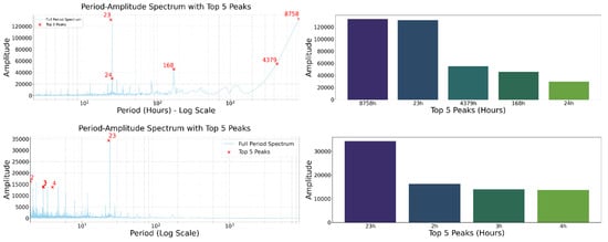
Figure 1.
FFT analyses and peak identification on the original (top) and first-differenced (bottom) series. Dominant periods from the differenced spectrum (e.g., in 15 min units) are adopted as model window sizes.

Table 1.
Dominant periods from FFT (top-K, in hours).
2.2.4. Implications for Window Design
Differenced peaks at {5, 12, 24} h suggest capturing (i) short transients (≤half-shift), (ii) shift transitions (≈half-day), and (iii) daily cycles. We therefore cover these timescales with (15 min units), which reduces exhaustive window search while preserving representational fidelity.
2.3. USAD with CNN–GRU Backbone
Building upon the FFT-guided multi-window configuration introduced in the previous subsection, this subsection details the USAD-based encoder–decoder instantiated with a CNN–GRU backbone for each selected window size. This subsection introduces an FFT-guided strategy for configuring multiple modeling windows, which forms a critical bridge between the data characteristics and the downstream encoder design. By selecting data-adaptive temporal scales, the proposed framework avoids reliance on a single, manually chosen window size that may fail to capture anomalies occurring at different time horizons. USAD comprises one encoder E and two decoders . For a standardized window ,
Phase 1 (reconstruction). Train and to minimize
Phase 2 (adversarial refinement). Encourage to make close to while separates them:
Backbone. The encoder stacks lightweight 1D CNN blocks (GELU activations) to capture local motifs, followed by a GRU bottleneck (hidden size d) to summarize the temporal context; decoders mirror the encoder with transposed convolutions/upsampling.
The detailed encoder–decoder configuration used for all window sizes is summarized in Table 2.
Table 2.
Encoder/decoder architecture (per window). All convolutions are 1D with GELU activations; LayerNorm after each block.
USAD is chosen for its ability to amplify subtle reconstruction discrepancies through adversarial refinement, which is particularly beneficial when downstream decision thresholds are learned without anomaly labels.
2.3.1. Training Schedule
We use Adam (), batch size 256 windows, and early stopping on validation loss with a patience of 10 epochs. Phase 1 runs for up to 50 epochs minimizing ; Phase 2 runs for up to 50 epochs on with a 1:1 alternation between and updates. Loss weights are fixed (), and gradient norms are clipped at 5. We seed all RNGs (42) and report medians over three independent runs.
2.3.2. Regularization
A light Dropout () after the GRU and weight decay () reduce overfitting on shorter windows; no data augmentation is used in the main results.
Figure 2 illustrates the overall FFT-guided multi-window USAD–DTW pipeline, including the two-phase USAD workflow. The complete training and inference procedure is formally described in Algorithm 1.
Algorithm 1 FFT-guided USAD–DTW with n-of-M aggregation. |
|
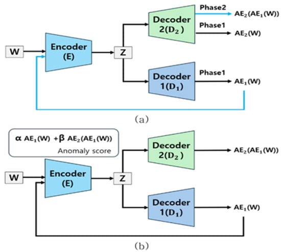
Figure 2.
Overall pipeline: raw series → FFT on differenced data → top-K periods → USAD-GRU per-window → reconstruction distance (DTW: optionally ) → Isolation Forest →n-of-M aggregation. (a) USAD Phase 1 architecture, (b) USAD Phase 2 architecture.
2.3.3. Why DTW + IF
Elastic alignment (DTW) mitigates phase jitter between observed and reconstructed windows, avoiding spurious penalties for small temporal shifts. Isolation Forest then replaces hand-tuned cutoffs with a data-adaptive decision rule that scales to streaming scenarios without labels.
2.3.4. Design Trade-Offs
A wider Sakoe–Chiba band (r) increases alignment tolerance but raises compute; a narrower band is faster but more sensitive to temporal drift. In practice, we use , which preserves recall under moderate jitter while keeping per-window complexity acceptable.
2.4. DTW Scoring, Aggregation, and Postprocessing
At inference, we measure reconstruction dissimilarities with Dynamic Time Warping (DTW). For sequences and local cost ,
where is a monotone warping path constrained by a Sakoe–Chiba band of width r (complexity ). We compute
and form the final score , .
2.4.1. Path-Length Normalization
To reduce dependence on path length, we also track normalized costs and , where is the cardinality of the optimal path. Unless otherwise noted, results use the unnormalized score S; normalized scores exhibited similar ranking in our dataset.
2.4.2. Aggregation and Tie-Breaking
Let . A timestamp is flagged when at least n of the M window-specific decisions are positive; we use and break ties toward the negative class to reduce spurious bursts. Postprocessing dilates window hits to point-level timestamps (15 min grid), merges adjacent hits with gap min, and drops events shorter than two points.
2.4.3. Computational Notes
DTW uses a Sakoe–Chiba band with width ; complexity per window is . We enable early abandoning when partial path costs exceed the current best, which reduces average runtime without affecting exactness under band constraints.
An Isolation Forest is fitted on observed under normal operation; final decisions are aggregated across windows via n-of-M voting. For evaluation at the point level, each window-level detection is dilated to all covered timestamps (15 min resolution), and then adjacent hits (gap ≤ 30 min) are merged and events shorter than two points are discarded.
2.5. Hyperparameters and Complexity Notes
Unless otherwise noted, stride , , , GRU hidden size , Adam learning rate , and seed 42, . FFT peak picking is , GRU inference is , and DTW with band r is per window. The default hyperparameter settings used throughout the experiments are listed in Table 3.
Table 3.
Default hyperparameters used in experiments.
2.5.1. Latency and Throughput
Let be the per-window DTW cost with constant determined by implementation and hardware. Total inference cost per timestamp is ; with and , the DTW term dominates for larger w while remaining within near-real-time budgets on commodity CPUs in our site. Batching across windows amortizes encoder/decoder calls; Isolation Forest adds negligible overhead at inference once fitted.
2.5.2. Tuning Knobs
Deployment-facing knobs are limited to contamination (IF), r (DTW band ratio), and n (aggregation). We scan , fix , and choose based on validation; this grid is small enough for routine recalibration. Limiting the number of tunable parameters reduces operational burden and facilitates deployment in settings where labeled anomalies are unavailable.
2.6. Evaluation Protocol (Point-Level with Window Dilation)
We evaluate detections at the point level by dilating each window-level detection to all timestamps covered by that window (15 min resolution). We merge adjacent hits (gap ≤ 30 min) and discard short events (<2 points). Hyperparameters are tuned on validation: contamination , DTW band ratio , and n-of-M aggregation ; we report test results using the best .
2.6.1. Split and Grid Search Protocol
We use chronological splits (2016–2019 for training/validation, 2019 for testing in our default setup). Hyperparameters are selected on validation only and then locked for test. All metrics are computed at the point level after dilation/merging. We report the best on validation and apply it unchanged to the test period.
2.6.2. Reproducibility
We record package versions (Python 3.10, PyTorch 2.x) and release configuration files containing , r, , n, and seeds. Randomness arises from weight initialization, batch ordering, and IF subsampling; we mitigate it by fixed seeds and by reporting medians over three runs.
3. Results
3.1. Detection Performance
We first evaluate the proposed method against representative unsupervised, reconstruction-based baselines to assess the benefit of FFT-guided multi-window modeling under a fully unlabeled setting. Our FFT-guided multi-window USAD–GRU with DTW/IF achieves F1 = 0.2060 and PR-AUC = 0.0923, with a precision of 0.1600 and a recall of 0.2892. Compared with single-window baselines (GRU-AE: F1 = 0.0323; Linear AE: F1 = 0.0350), our method yields a relative F1 improvement of 489%. We evaluate at the point level by dilating each window-level detection to its covered timestamps and applying a minimum event-length filter of length points. Given the extreme class imbalance in industrial streams, we prioritize PR–AUC over ROC–AUC, as the latter can be overly optimistic under rare-event conditions.
Beyond the single operating point, we examine threshold-free behavior via PR–AUC, which is for our method versus near-zero for single-window baselines. In highly imbalanced streams, PR–AUC is a more faithful indicator of practical utility than ROC–AUC, and the observed gap implies that our ensemble maintains precision in the low-recall regime while recovering recall as the threshold is relaxed. Importantly, the gains persist when we vary the minimum event-length filter from 2 to 5 points, indicating that improvements are not merely due to aggressive postprocessing.
Ablation on window participation further clarifies the source of gains: short windows (e.g., ) capture abrupt spikes from switching operations, whereas longer windows () capture slow drifts and regime transitions. The n-of-M aggregation attenuates idiosyncratic errors from any single scale and produces more stable decisions over calendar boundaries (e.g., month-end load reshaping). To avoid optimistic bias, we report point-level metrics after dilating window-level hits to their covered timestamps, which penalizes fragmented detections and aligns with plant-floor alerting practice. For transparency, the “489%” relative F1 improvement is computed as , using the strongest single-window baseline (Linear AE, F1) as the reference. While absolute F1 remains modest due to label sparsity and mixed periodicities, the relative lift is operationally meaningful: with the same alert budget, the ensemble surfaces more true events and reduces weekend/night artifacts. We note that comparisons with supervised detectors, which have access to labeled anomalies, are deferred to a subsequent subsection to contextualize performance trade-offs between supervised and fully unsupervised settings.
We compared our method with a state-of-the-art Transformer-based autoencoder. Despite its high complexity, it failed to capture the diverse periodic patterns effectively in this unsupervised setting (Table 4).
Table 4.
Detection performance on the target dataset. The Transformer AE baseline is included to highlight the effectiveness of the proposed multi-window approach.
3.2. Ablation on , r, and n-of-M
We analyze the sensitivity of the proposed pipeline to key deployment-facing hyperparameters, namely the IF contamination , the DTW band ratio r, and the aggregation rule n-of-M. Recall increases with larger and union aggregation (), while precision improves with and longer event filters. We select to maximize F1 on validation.
The loss-weight controls the strength of adversarial regularization in USAD. A larger encourages conservative reconstructions and increases recall by widening the margin between normal and abnormal patterns; however, excessive values oversmooth local motifs and reduce precision. The DTW band ratio r governs boundary refinement and latency: smaller r tightens the alignment and favors precision, while larger r relaxes the alignment and improves recall near regime changes, at the cost of higher compute.
Aggregation exhibits the expected trade-off. Union () maximizes coverage and is useful for forensic review, whereas majority () suppresses scale-specific noise and yields higher precision under mixed periodicities. On validation splits, we found that typically pairs with , indicating that a modest consensus is sufficient to stabilize decisions without sacrificing the complementary strengths of short and long windows. These trends persist across alternative elbow thresholds and event-length filters, suggesting that the gains are not hyperparameter-brittle.
Figure 3 illustrates the sensitivity analysis results. Interestingly, the performance drops significantly for majority voting (), indicating that anomalies detected at different temporal scales are mutually exclusive. This strongly justifies our adoption of the union aggregation strategy ().
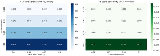
Figure 3.
Parameter sensitivity analysis for contamination (), DTW band width (r), and aggregation (n). The heatmap indicates that union-based aggregation () yields higher sensitivity (recall) and F1 scores compared to majority voting (), and the performance remains stable across a reasonable range of DTW band widths.
3.3. Operational Efficiency
Table 5 reports inference latency per window with a Sakoe–Chiba band () and stride , remaining compatible with a 15 min sampling cadence. Latency grows approximately linearly with the window length, remaining comfortably within a 15 min sampling cadence even for . Because DTW with a Sakoe–Chiba band scales as in both time and memory, choosing limits overhead while preserving boundary sensitivity. In deployment, window branches can be parallelized across cores/GPUs and DTW evaluations can be batched, keeping end-to-end wall-clock time near the slowest branch rather than the sum. This profile enables near-real-time triage and periodic re-estimation of spectral peaks without disrupting ongoing inference.
Table 5.
Inference latency per window (15 min sampling).
3.4. Clustering and Operational Insights
We cluster daily profiles (96-slot vectors) and obtain K clusters. Cluster-wise averages reveal shift/day–night regimes and weekend patterns (Figure 4); Table 6 summarizes the days per cluster. Daily-profile clustering reveals distinct operating regimes that align with shift start/stop, lunch breaks, and weekend schedules. Clusters with sharp morning ramp-ups are correlated with higher anomaly rates during early hours, while flatter clusters concentrate residual alerts around maintenance windows. These regimes explain a portion of the spectral energy near daily harmonics and motivate keeping multiple window sizes during training. They also inform hour- and mode-conditioned thresholds, which reduced false positives in validation by suppressing alerts during predictable high-variance periods.
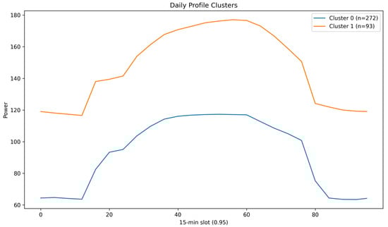
Figure 4.
Cluster-wise average daily profiles (96-slot vectors).
Table 6.
Daily-profile clustering summary (days per cluster).
We then group anomaly events using length/shape/temporal features (PCA–2D in Figure 5); Table 7 shows that short bursts and longer drifts form distinct types with different hour/day-of-week preferences. Event-level clustering corroborates two dominant types: short bursts with steep onsets (often linked to switching or brief overloads) and longer drifts (linked to calibration issues or gradual fouling). The separation suggests different response playbooks: rapid operator confirmation for bursts versus preventive maintenance tickets for drifts. Embedding these priors into alarm routing can shorten time-to-action without changing the underlying detector.
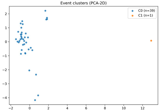
Figure 5.
Event-level clustering in PCA–2D space.
Table 7.
Event-level clustering summary.
Finally, hour-of-day/day-of-week analyses (Figure 6) motivate hour-adaptive thresholds in deployment. A clear weekly rhythm appears, with elevated loads during weekday daytime and reduced activity overnight and on weekends. Hours with consistently high variance are also periods where false positives are more likely if a single threshold is used; schedule-aware thresholds and periodic peak re-estimation help mitigate this issue.
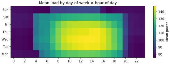
Figure 6.
Mean load by day-of-week and hour-of-day.
3.5. Qualitative and Error Analysis
Figure 7 shows the full period with detected anomalies; a one-month zoom is provided in Figure 8. We observe that multi-window aggregation reduces night/weekend false positives while retaining abrupt spikes and slow drifts. Visual inspection over the full period shows that the ensemble suppresses many night/weekend artifacts while retaining operationally meaningful events. The one-month zoom highlights boundary handling: DTW-based smoothing merges fragmented hits across short gaps, and the minimum event-length filter removes transient blips. Remaining false positives are mostly attributable to scheduled tests and sensor dropouts; both can be mitigated by excluding known maintenance windows and by down-weighting channels with intermittent missingness.
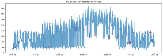
Figure 7.
Full period with detected anomalies (red markers) after window-to-point dilation and event filtering.
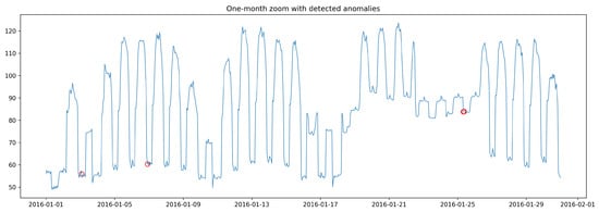
Figure 8.
One-month zoom with detected anomalies. Red circles indicate timestamps flagged as anomalous after window-to-point dilation and post-processing (merging and minimum event-length filtering). Union () vs. majority () aggregation yields a precision–recall trade-off.
Typical failure modes include borderline oscillations near setpoint changes and slow drifts that exceed the longest window only after several days. A simple remedy is to append a coarser weekly window to the ensemble or to incorporate an exponential moving average of scores for slow-trend tracking. We leave this extension to future work, as the current design already meets latency and precision requirements for plant-floor monitoring.
4. Discussion
FFT-guided windowing aligns model capacity with site-specific rhythms, while the two-phase USAD training tightens the normal region by contrasting reconstructions. DTW-based scoring reduces sensitivity to phase jitter and minor timing shifts, and Isolation Forest provides fast, nonparametric decisions without manual threshold tuning. Together, these choices form a deployment-oriented pipeline that preserves robustness under mixed periodicities and nonstationary regimes. Beyond individual components, the proposed framework is designed around the principle of data-adaptive simplicity: rather than increasing model depth or task-specific supervision, we align representation scales with site-specific rhythms and enforce robustness at the scoring stage. This design choice prioritizes stable operation under nonstationarity and mixed periodicities, which are common in industrial environments but rarely satisfied by off-the-shelf detectors.
4.1. Unsupervised vs. Supervised Detectors
While supervised detectors generally achieve higher absolute performance when abundant labeled anomalies are available, their applicability in industrial monitoring is often limited by annotation cost, label sparsity, and concept drift. In our experiments, supervised baselines achieve higher peak F1 under controlled conditions, but require frequent re-labeling and retraining to maintain performance across calendar and regime changes.
In contrast, the proposed method operates fully unsupervised and emphasizes robustness and deployability. Although absolute F1 remains modest, the relative improvement over unsupervised baselines and the stability under temporal shifts suggest that the method is better suited for continuous monitoring scenarios where labels are scarce or nonstationary.
4.2. Practical Implications
The proposed design depends only on unsupervised data and uses standard components (FFT, 1D CNN/GRU, DTW, Isolation Forest), which simplifies integration into existing monitoring stacks. FFT-guided windowing yields a compact set of models covering sub-daily to daily cycles, avoiding exhaustive window searches. DTW scores can be inspected at the point level to localize abnormal segments within a window, which is useful for triage and operator feedback. As a result, the framework can be incrementally deployed and calibrated without disrupting existing alerting pipelines or requiring labeled anomaly archives.
4.3. Limitations and Threats to Validity
First, window-specific hyperparameters (e.g., DTW band width, GRU size, score mixing ) introduce tuning overhead, and poorly chosen parameters may inflate latency or false alarms. Second, purely unsupervised scores can drift under long-term distribution shifts, especially when operating schedules change. Third, DTW—even with banding—adds per-window cost that grows with window length; real-time use requires careful selection of r and model pruning. Finally, results are from a single industrial site; external validity to other plants and load regimes must be established.
4.4. Operational Considerations
In production, we recommend the following: (i) periodic re-estimation of FFT peaks when operating schedules change; (ii) light human-in-the-loop calibration using a small, curated set of confirmed events to stabilize Isolation Forest contamination; and (iii) watchdogs for score drift (e.g., population shift tests on S) to trigger retraining.
4.5. Future Work
Future directions include multi-site validation with heterogeneous schedules, attribution methods using segment-level DTW cost heatmaps for explainability, adaptive window management (adding/removing windows as spectra evolve), and closed-loop integration with maintenance systems for automated ticketing and prioritization.
5. Conclusions
We presented a practical, unsupervised framework for anomaly detection in industrial power time-series that combines FFT-guided multi-window modeling, a USAD architecture with a CNN–GRU backbone, DTW-aware scoring, and Isolation Forest decisions. On a single-site, three-year dataset, the method robustly captures spikes and drifts across sub-daily to daily timescales and is amenable to near-real-time deployment. The design choices emphasize interpretability (via spectral guidance and DTW cost inspection) and operational simplicity, offering a viable path to scalable monitoring in smart-factory environments.
Author Contributions
Conceptualization, W.K., J.P. and S.L.; methodology, W.K., J.P., M.J. and S.L.; software, W.K., J.P. and M.J.; validation, M.J. and S.L.; writing—original draft preparation, W.K. and J.P.; writing—review and editing, S.L.; supervision, S.L.; project administration, S.L. All authors have read and agreed to the published version of the manuscript.
Funding
This research was supported by the Regional Innovation System & Education (RISE) Program through the Daejeon RISE Center, funded by the Ministry of Education (MOE) and Daejeon Metropolitan City, Republic of Korea (Grant No. 2025-RISE-06-002).
Data Availability Statement
Data are not publicly available due to industrial confidentiality.
Acknowledgments
The authors thank the Daejeon RISE Center for administrative support and ETRI colleagues for valuable technical discussions.
Conflicts of Interest
The authors declare no conflicts of interest.
References
- Chandola, V.; Banerjee, A.; Kumar, V. Anomaly Detection: A Survey. ACM Comput. Surv. 2009, 41, 1–58. [Google Scholar] [CrossRef]
- Aggarwal, C.C. Outlier Analysis; Springer: Berlin/Heidelberg, Germany, 2017. [Google Scholar]
- Hyndman, R.J.; Athanasopoulos, G. Forecasting: Principles and Practice; OTexts: Melbourne, Australia, 2018. [Google Scholar]
- Lee, J.; Bagheri, B.; Kao, H.A. A Cyber–Physical Systems Architecture for Industry 4.0-Based Manufacturing Systems. Manuf. Lett. 2015, 3, 18–23. [Google Scholar] [CrossRef]
- Syafrudin, M.; Alfian, G.; Fitriyani, N.L.; Rhee, J. Performance analysis of IoT-based sensor, big data processing, and machine learning model for real-time monitoring system in automotive manufacturing. Sensors 2018, 18, 2946. [Google Scholar] [CrossRef] [PubMed]
- Oppenheim, A.V.; Schafer, R.W. Discrete-Time Signal Processing; Prentice Hall: Upper Saddle River, NJ, USA, 1999. [Google Scholar]
- Hendrycks, D.; Gimpel, K. Gaussian Error Linear Units (GELUs). arXiv 2016, arXiv:1606.08415. [Google Scholar]
- Audibert, J.; Michiardi, P.; Guyard, F.; Marti, S.; Zuluaga, M.A. USAD: Unsupervised Anomaly Detection on Multivariate Time Series with Attentional Autoencoders. In Proceedings of the 26th ACM SIGKDD International Conference on Knowledge Discovery & Data Mining (KDD), Virtual, 6–10 July 2020; ACM: New York, NY, USA, 2020. [Google Scholar]
- Cho, K.; van Merrienboer, B.; Gulcehre, C.; Bahdanau, D.; Bougares, F.; Schwenk, H.; Bengio, Y. Learning Phrase Representations using RNN Encoder–Decoder for Statistical Machine Translation. arXiv 2014, arXiv:1406.1078. [Google Scholar]
- Kim, Y. Convolutional Neural Networks for Sentence Classification. In Proccedings of the Conference on Empirical Methods in Natural Language Processing (EMNLP), Doha, Qatar, 25–29 October 2014; ACL: Austin, TX, USA, 2014. [Google Scholar]
- Sakoe, H.; Chiba, S. Dynamic programming algorithm optimization for spoken word recognition. IEEE Trans. Acoust. Speech Signal Process. 1978, 26, 43–49. [Google Scholar] [CrossRef]
- Liu, F.T.; Ting, K.M.; Zhou, Z.-H. Isolation Forest. In Proceedings of the 2008 Eighth IEEE International Conference on Data Mining; IEEE: New York, NY, USA, 2008; pp. 413–422. [Google Scholar]
- Berndt, D.J.; Clifford, J. Using Dynamic Time Warping to Find Patterns in Time Series. In Proceedings of the KDD Workshop, Newport Beach, CA, USA, 14–17 August 1997; pp. 229–242. [Google Scholar]
- Xu, H.; Chen, W.; Zhao, N.; Li, Z.; Bu, J.; Li, Z.; Liu, Y.; Zhao, Y.; Pei, D.; Feng, Y.; et al. Unsupervised anomaly detection via variational auto-encoder for seasonal KPIs in web applications. In Proceedings of the 2018 World Wide Web Conference, Geneva, Switzerland, 10 April 2018; pp. 187–196. [Google Scholar]
- Malhotra, P.; Ramakrishnan, A.; Anand, G.; Vig, L.; Agarwal, P.; Shroff, G. LSTM-Based Encoder–Decoder for Anomaly Detection in Time Series. arXiv 2016, arXiv:1607.00148. [Google Scholar]
- Park, D.; Hoshi, T.; Kawahara, Y. A Time-Series Anomaly Detection Method Based on a Variational Autoencoder. IEICE Trans. Inf. Syst. 2018, E101.D, 2110–2119. [Google Scholar]
- Schmidhuber, J. Deep Learning in Neural Networks: An Overview. Neural Netw. 2015, 61, 85–117. [Google Scholar] [CrossRef] [PubMed]
- Jung, M.; Jang, H.; Kwon, W.; Seo, J.; Park, S.; Park, B.; Park, J.; Yu, D.; Lee, S. A Comparative Study of Customized Algorithms for Anomaly Detection in Industry-Specific Power Data. Energies 2025, 18, 3720. [Google Scholar] [CrossRef]
- Backhus, J.; Rao, A.R.; Venkatraman, C.; Gupta, C. Time Series Anomaly Detection Using Signal Processing and Deep Learning. Appl. Sci. 2025, 15, 6254. [Google Scholar] [CrossRef]
- Sun, Y.; Liang, M.; Zhang, S.; Che, Z.; Luo, Z.; Li, D.; Zhang, Y.; Pei, D.; Pan, L.; Hou, L. Efficient Multivariate Time Series Anomaly Detection through Transfer Learning for Large-Scale Software Systems. ACM Trans. Softw. Eng. Methodol. 2025, 34, 984. [Google Scholar] [CrossRef]
- Song, Y.; Kuang, S.; Huang, J.; Zhang, D. Unsupervised Anomaly Detection of Industrial Building Energy Consumption. Energy Built Environ. 2024; in press. [Google Scholar] [CrossRef]
- Kingma, D.P.; Ba, J. Adam: A Method for Stochastic Optimization. arXiv 2014, arXiv:1412.6980. [Google Scholar]
Disclaimer/Publisher’s Note: The statements, opinions and data contained in all publications are solely those of the individual author(s) and contributor(s) and not of MDPI and/or the editor(s). MDPI and/or the editor(s) disclaim responsibility for any injury to people or property resulting from any ideas, methods, instructions or products referred to in the content. |
© 2025 by the authors. Licensee MDPI, Basel, Switzerland. This article is an open access article distributed under the terms and conditions of the Creative Commons Attribution (CC BY) license (https://creativecommons.org/licenses/by/4.0/).