Interaction Analysis of Offshore Power Systems: A Comparative Study

Abstract

This paper presents a comparative assessment of interaction analysis methods applied to a multi-variant offshore power system model. Complementary analytical techniques—eigenvalue analysis, frequency–response characteristics, RGA, DRGA, and GDRG—are used to quantify interactions across electromechanical and electromagnetic frequency ranges. The main novelty of this study is a modified DRGA approach that incorporates a hybrid FIR/IIR digital filtering stage, significantly improving the accuracy of interaction evaluations. The results show that no single method provides complete data and that the enhanced DRGA and GDRG techniques are essential for interaction analysis. The proposed framework offers practical guidelines for analyzing and coordinating control loops in offshore grids.

1. Introduction

The growing demand for renewable energy and limited availability of land-based resources have increased the importance of offshore power systems. The use of offshore areas is also essential for achieving climate and decarbonization targets [1]. Recent technological progress has significantly expanded the potential of offshore grids, combining the increasing capacity of wind turbines with the development of new technologies for harnessing energy from ocean waves and sea currents [2]. The development of the wind generation sector and its impact on power system operation, as demonstrated in [3], further emphasize the challenges and opportunities linked to integrating large-scale renewable sources. According to [4,5], around 8 GW of new offshore wind capacity was added in 2024, bringing the total installed capacity to 83 GW by the end of the year. Although this represents continued steady growth, it was actually lower than the record 10.8 GW added in 2023 [6]. Most new wind power installations in 2024 were onshore (109 GW of the total 117 GW added), while the offshore sector continued to scale up steadily [7]. Predictions indicate that annual offshore wind installations will rise from around 8 GW in 2024 to about 34 GW by 2030, representing an increasing share of global wind deployment [8]. According to forecasts by [9,10], total installed offshore wind capacity is expected to reach 258 GW by 2030. However, analyses by [11] highlight that, to achieve the 1.5 °C target, as much as 494 GW of offshore wind would be required globally by 2030, rising to more than 2400 GW by 2050. These figures demonstrate both the rapid growth and the scale of the challenge facing the offshore sector.

The European Union (EU) aims for climate neutrality by 2050, which requires significant investments in renewable energy sources, particularly those located in offshore areas, as well as the development of grid infrastructure. The EU targets 100 GW of offshore wind by 2030 and 300 GW by 2050, supported by initiatives such as offshore hybrid projects and meshed offshore grids. Achieving these objectives requires not only technological innovation but also stable and reliable integration of offshore resources with onshore power systems.

The continued development of the power system will result in a growing number of control systems, which may cause undesirable interactions affecting system stability and reliability [5]. The use of renewable energy sources, where individual generating units are equipped with controllers or operate under centralized control (e.g., in the case of wind farms), highlights the need to determine appropriate control signals and analyze interactions between different control systems. A technical challenge arises from the growing penetration of power electronic converters in offshore systems. Offshore wind turbines, wave energy converters, and tidal or marine current units are typically connected through converter-based interfaces, which provide operational flexibility but may also introduce negative interactions.

Despite the use of advanced controller design and parameter tuning methods, interactions between controllers cannot be completely avoided [12]. To address the problem of interactions, various methods for their detection and analysis are being developed. These methods make it possible to identify the sources and causes of interactions and can also be useful for modifying the control structure. Control systems can be designed using either centralized or decentralized approaches. Decentralized control systems are still used in most applications, mainly due to their simpler implementation, operation, and tuning. The main stages in the operation of decentralized controllers can be divided into the following steps [13]:

• Determination of control objectives and system models;
• Selection of control structure;
• Interaction analysis;
• Controller design;
• Simulations, experimental validation, and implementation.

The selection of the control structure is an important issue, as it has a significant impact on the proper operation of the system. This process can be divided into two main steps:

• Selection of input and output signals;
• Selection of the control configuration, including the input–output pairing problem.

The main objective in selecting an appropriate control structure is to achieve the desired control objectives while minimizing interactions between control loops.

The presence of multiple control systems can result in oscillations, reduced damping, or even instability when these units are integrated into large-scale offshore grids [5]. Consequently, understanding the interaction phenomena among different offshore generation technologies, as well as between offshore systems and onshore grids, is essential for the design of reliable future power systems.

The main objective of this paper is to demonstrate how different interaction analysis methods can complement each other within a proposed offshore grid test model. The paper further illustrates the application of several complementary methods—the sensitivity analysis based on eigenvalues and participation factors, frequency response characteristics and interaction measures such as relative gain array (RGA), dynamic relative gain array (DRGA), and generalized dynamic relative gain (GDRG). By integrating these techniques, the study provides a comprehensive framework for identifying, quantifying, and comparing interactions between system components under various operating conditions, offering a better understanding of system dynamics and control coordination.

This study aims to contribute to the field of interaction analysis in power systems. It presents a comprehensive overview and application of analytical (non-simulation-based) interaction analysis methods, highlighting their individual usefulness, mutual complementarity, and the way they can be used to achieve a more complete assessment of system interactions. Furthermore, the DRGA method has been improved by introducing an additional digital filtering stage, which enhances the accuracy of the obtained results. Finally, the developed analytical framework has been applied to a test model of an offshore power system to evaluate its performance and demonstrate the applicability of the proposed approach.

The remainder of this paper is organized as follows. Section 2 presents the background and related work on offshore grids and interaction phenomena in power systems. Section 3 outlines the main characteristics of offshore power systems, while Section 4 introduces the modelling approach. Section 5 defines the concept and objectives of interaction analysis and describes the methods considered in this study. Section 6 presents and discusses the results of the interaction analysis. Finally, the paper is concluded with a summary.

2. Background and Related Work

From the control theory point of view, the power system can be regarded as a multiple-input, multiple-output (MIMO) system. A single control input may negatively affect other output signals, which is why the selection of input–output pairs should be performed in a way that minimizes negative interactions and ensures overall system stability [14]. Such interactions may arise not only between controllers but also among individual components of the power system. In the context of long-term power system development, this issue becomes even more relevant [15]. Many studies—including those in Europe indicate that offshore renewable energy technologies, especially offshore wind, will play a central role in achieving very high or even 100% renewable energy penetration by 2050. Long-term planning models consistently show that offshore capacity is critical for meeting decarbonisation targets, reducing land-use constraints, and achieving system adequacy in low-carbon scenarios [16]. However, these studies typically rely on simplified representations of offshore generation and do not capture the detailed dynamic interactions between offshore controllers, grid-forming units, and transmission systems. As a result, the operability and dynamic stability of the future energy mix largely dependent on offshore infrastructure remain insufficiently explored.

Traditional power-system stability tools provide valuable insights into individual modes of oscillation or component behaviour but often fail to fully characterize the interactions between multiple control loops. For example, interactions between power system stabilizers (PSS) and flexible AC transmission systems (FACTSs) have long been recognized [17], where the controller of one device may influence another and reduce system damping [5]. In high-voltage direct-current (HVDC) transmission, rectifier control loops may interact with turbine–generator units [18], impacting voltage and transient stability [19]. Similar challenges arise in large offshore wind farms, where numerous converter-interfaced turbines can interact through the grid and exhibit low-frequency oscillations [20].

Doubly fed induction generators (DFIGs) are sensitive to sub-synchronous control interactions (SSCIs), a form of sub-synchronous resonance (SSR) [21,22]. SSCIs may occur between DFIG-based wind farms and series-compensated AC networks [23,24]. Wind farms based on permanent-magnet synchronous generators (PMSGs) exhibit related issues, particularly when reactive-power compensation devices are present [23,25]. Furthermore, PMSG-based turbines may interact with HVDC systems—both line-commutated (LCC) and voltage-source (VSC) types—through sub-synchronous oscillations and coupled control loops [26,27].

To assess these interaction phenomena, a variety of analytical tools have been developed. The RGA remains one of the earliest and most frequently used methods [28], offering a static measure of input-output coupling at a given frequency. Its limitations have motivated the development of frequency-dependent extensions such as the DRGA and GDRG [29,30], which broaden the analysis to include frequency ranges relevant for electromechanical and control-driven oscillations. Alternative methods focus on impedance-based modelling, particularly in converter-dominated grids and HVDC systems. The authors in [31] proposed a dynamic modelling framework for multi-terminal HVDC systems, enabling impedance-based interaction analysis and stability assessment. Their results highlight the importance of interaction studies in offshore power systems. In [32], the authors outlined a method for analyzing harmonic interactions in wind farms. Sub-synchronous interactions in power systems with high wind penetration were investigated in [33], demonstrating the crucial role of controller tuning in preventing stability issues. A comprehensive review of offshore wind farm stability analysis methods was presented in [34], emphasizing the need to combine time- and frequency-domain approaches.

Previous studies have extensively examined the stability of offshore wind farms, addressing small-signal dynamics, frequency response behaviour, and interactions with HVDC transmission systems. Research has also investigated tidal and wave energy converters, as well as hybrid offshore configurations. However, most existing works focus on single-technology systems or specific aspects of integration. What remains largely unexplored is the dynamic interaction behaviour of multi-technology offshore systems, especially those expected to operate in future energy mixes dominated by converter-based generation and offshore infrastructure.

To address this research gap, the present study investigates interaction phenomena in offshore power systems comprising offshore wind farms, marine-current energy farms, synchronous-generator units, and offshore loads. Emphasis is placed on comparative evaluation of control-loop interactions and their influence on angular stability. The assessment combines several complementary techniques—RGA, DRGA, GDRG, eigenvalue analysis and frequency–response analysis. In doing so, the study contributes to a deeper understanding of future offshore grids and supports the operability of long-term renewable-energy scenarios in which offshore technologies are expected to play a critical role.

3. Offshore Power Systems

Offshore power systems represent an increasingly important component of modern and future electricity networks, driven by the rapid expansion of offshore wind energy and tidal and marine current technologies. These systems are no longer envisioned as isolated generation assets, but rather as integrated elements of broader onshore–offshore energy architectures. Their role is particularly significant in long-term scenarios, where offshore renewable resources are expected to provide a substantial share of the electricity required to meet 2050 decarbonisation targets.

Large-scale modelling efforts—such as [35] indicate that offshore wind must become a central pillar of future power systems to enable deep emissions reductions while maintaining reliability and affordability.

Global analyses further highlight that offshore renewable deployment is particularly critical in regions with limited land availability or high population density, such as Japan [36] and parts of Western Europe, where large-scale onshore wind and solar installations face geographical or environmental constraints [37]. In Latin America—where studies for Mexico [38] and Ecuador have explored least-cost 2050 transition pathways—offshore wind is identified as an important option for diversifying renewable supply and enhancing seasonal balancing [39]. Similarly, long-term planning assessments for South Africa and other coastal regions of Africa show that offshore resources can complement solar dominated [40].

Although offshore systems operate predominantly at sea, their development is closely linked to the evolution of onshore infrastructures. Recent studies show that hydropower reservoirs, coastal lagoons and artificial basins are increasingly being used not only for conventional hydro generation but also as platforms for floating photovoltaic (FPV) systems and hybrid wind–hydro–solar installation. The European Joint Research Centre has shown that installing FPV systems on water reservoirs can significantly increase overall renewable energy generation [41]. Likewise, comprehensive reviews indicate that reservoirs and coastal basins are well suited for hosting FPV installations in combination with wind generation, as their production profiles complement seasonal variations in wind output [42].

Due to the environmental conditions prevailing in offshore areas, transmission systems integrated into offshore power grids are based on submarine AC or direct current (DC) cable lines. In the early stages of offshore grid development, these systems primarily consisted of radial connections between offshore wind farms (OWF) and the onshore grid (Figure 1a) or were designed to connect two onshore power systems. The further development of offshore transmission networks is expected to increase the potential of existing infrastructure, leading to grids with more complex topologies. This concept assumes the construction of offshore hub stations that will serve both as connection points for distributed offshore wind farms and as nodes for export cables routed toward land (Figure 1b).

Figure 1. Typical stages in the development of offshore grids. EPS—equivalent power system, ONS—onshore substation, OFS—offshore substation, IL—industrial load, OWF—offshore wind farm. (a) radial offshore grid topology; (b) offshore hub substation topology with centralized export to onshore grid.

In Europe, such offshore power grids offer new possibilities for cross-border power exchange and system integration [43]. The increasing complexity of offshore transmission network topologies is accompanied by higher uncertainty related to system components parameters, and the variability of power generation or consumption, all of which impose additional challenges for system operation [44].

The integration of industrial loads (IL) is becoming an important element of future offshore grids. The North Sea region already demonstrates practical examples involving several large oil and gas platforms [45,46]. Beyond oil and gas electrification, offshore hydrogen production projects [47,48] show how renewable offshore power can directly feed such installations. At a broader scale, offshore energy islands are designed as hybrid hubs connecting wind farms with potential industrial facilities [49,50]. These initiatives signal a shift from generation-only offshore systems toward integrated energy-industry ecosystems supported by meshed grid architectures [51].

An important consideration in the design of offshore power systems is the technology used for transmission—AC or DC cable lines. Most existing offshore wind farms are located relatively close to shore; therefore, AC cable connections are typically employed, as there is no technical or economic justification for using DC connections in such cases. The fundamental difference between overhead lines and cable lines lies in their parameters—capacitance and inductance. The capacitance of a cable line can be several times higher than overhead line [52]. Consequently, for cable lines, the issue of capacitive current, also referred to as charging current, becomes particularly important. For a given line length, it may reach the cable’s thermal limit, thereby preventing the transmission of active power and, in practice, rendering the AC cable incapable of power transfer [53]. To mitigate the adverse effects of reactive power in AC cable lines, compensation devices are used. These can be installed in various configurations: at one end, at both ends, at both ends of a section, or at intermediate nodes along the cable.

If an offshore wind farm is located beyond the practical transmission range of AC lines, or if its rated power is particularly high, a HVDC link becomes a more suitable solution. For DC transmission, there is no defined length limitation [53]. HVDC technology is considered cost-effective for offshore cable connections longer than about 50–100 km [54]. This configuration requires converter stations at both ends of the transmission line, which may employ different converter topologies: LCC, VSC, capacitor-commutated converters (CCC) or current source converters (CSC) [55]. Among these technologies, VSC systems are most commonly used in offshore applications, primarily due to their ability to operate with a passive grid—i.e., in the absence of local voltage sources. The main drawbacks of this converter topology are its higher cost and limited bandwidth.

The development of offshore power systems—and particularly the simultaneous use of both transmission technologies, high voltage alternating current (HVAC) and HVDC, within one or more networks—has led to the concept of hybrid grids. This approach offers significant opportunities to reduce the loading of AC lines, improve the utilization of existing infrastructure, and lower overall costs [56]. A complete transition to direct current transmission technologies is unlikely from a technical perspective. Therefore, research on hybrid grids focuses on combining the advantages of both transmission technologies to increase transfer capacity, interconnect systems operating at different frequencies, and improve the efficiency of long-distance power transmission [57].

4. Offshore Test System Modelling

4.1. Mathematical Background

The objective of the study is to evaluate and compare interaction analysis methods rather than to assess the performance of a particular real-world installation. Since the analyzed phenomena arise from general system characteristics rather than site-specific details, the proposed model ensures that the conclusions regarding methods remain valid for practical offshore systems. The behaviour of dynamic systems such as power system can be described using a set of first-order nonlinear equations, given in (1) [58]:

$${\dot{x}}_i=f_i\left(x_1,x_2,\dots ,x_n;u_1,u_2,\dots ,u_r;t\right) i=\mathrm{1,2},\dots ,n$$

(1)

where $n$ denotes the order of the system, and $r$ denotes the number of inputs. Equation (1) can also be expressed in a vector-matrix form shown in (2):

$$\dot{\mathbf{x}}=\mathbf{f}\left(\mathbf{x},\mathbf{u},t\right)$$

(2)

With the state, input and function vectors defined in (3):

$$\mathbf{x}=\left[\begin{array}{c}{x}_1\\ x_2\\ ⋮\\ x_n\end{array}\right] \mathbf{u}=\left[\begin{array}{c}{u}_1\\ u_2\\ ⋮\\ u_r\end{array}\right] \mathbf{f}=\left[\begin{array}{c}{f}_1\\ f_2\\ ⋮\\ f_n\end{array}\right]$$

(3)

The column vector $\mathbf{x}$ is referred to as the state vector, and its elements are state variables. The column vector $\mathbf{u}$ is referred to as the input vector, representing external signals that affect the operation of the system. Time is denoted by $t$ and the time derivative of state vector $\mathbf{x}$ is denoted as $\dot{\mathbf{x}}$. If state variables are not functions of time, the system is considered as stationary. Two types of dynamic models are used to analyze interactions that affect the stability of the power system: nonlinear and linear.

A nonlinear model can be expressed using differential-algebraic Equations (4) and (5) [46]:

$$\dot{\mathbf{x}}=\mathbf{f}\left(\mathbf{x},\mathbf{u}\right)$$

(4)

$$\mathit{y}=\mathbf{g}\left(\mathbf{x},\mathbf{u}\right)$$

(5)

where $\mathbf{f}\left(\mathbf{x},\mathbf{u}\right)$ and $\mathbf{g}\left(\mathbf{x},\mathbf{u}\right)$ are vectors of nonlinear functions and $\mathit{y}$ is the vector of output signals.

A linear model, commonly used in the analysis of interactions between control loops and subsystems, can be derived by linearizing Equations (4) and (5) around an operating point. This model can be expressed in (6) and (7):

$$∆\dot{\mathbf{x}}=\mathbf{A}∆\mathbf{x}+\mathbf{B}∆\mathbf{u}$$

(6)

$$∆\mathbf{y}=\mathbf{C}∆\mathbf{x}+\mathbf{D}∆\mathbf{u}$$

(7)

where $∆\mathbf{x}$—state vector of dimension $n$, $∆\mathbf{y}$—output vector of dimension $m$, $∆\mathbf{u}$—input vector of dimension $r$, $\mathbf{A}$—system (state) matrix of size $n\times n$, $\mathbf{B}$—control matrix of size $n\times r$, $\mathbf{C}$—output matrix of size $m\times n$, $\mathbf{D}$—transmission matrix of size $m\times r$.

4.2. Properties of the Test System

For the purpose of this study, an offshore power system model illustrated in Figure 2 was proposed.

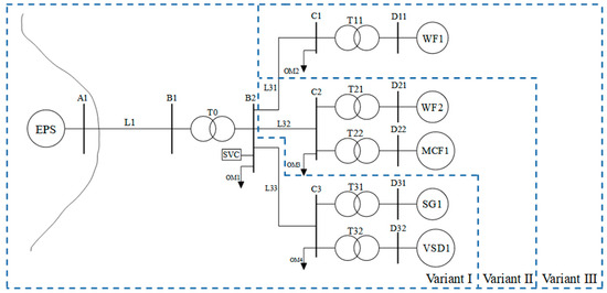
Figure 2. Schematic diagram of the offshore power system test model.

The test system model was designed as a universal model representing typical configurations and technologies of offshore power systems. Although it is not a direct representation of a specific industrial installation, the model incorporates elements commonly found in real engineering practice.

The developed test model includes 110 kV and 33 kV submarine cables. The individual components of the system are interconnected through six electrical nodes. The 110 kV transmission line connects the onshore grid (node A1) with the offshore substation (node B1). A Static Var Compensator (SVC) and a local static load (OM1) are connected at node B1. The offshore substation includes transformer T0, with a voltage ratio of 110/33 kV, and its low-voltage side is connected to node B2. From this substation, three 33 kV lines (L31, L32, and L33) connect the offshore substation with other elements of the system. The offshore wind farms and the marine farm were aggregated to simplify the analysis and are represented by equivalent models—in this case, by DFIG and PMSG generator models, respectively. The developed test model of the offshore power system consists of the following components:

• onshore equivalent power system operating at 110 kV (EPS),
• 110 kV transmission line (line L1),
• 110/33 kV transformer (transformer T0),
• 33 kV transmission lines (lines L31, L32, and L33),
• 33/0.69 kV transformers (transformers T11, T21, and T22),
• 33/6.6 kV transformer (transformer T32),
• 33/10.5 kV transformer (transformer T33),
• static loads (OM1, OM2, OM3, and OM4),
• Static Var Compensator (SVC),
• offshore wind farm (WF1) rated at 50 MW,
• offshore wind farm (WF2) rated at 50 MW,
• marine current farm (MCF1) rated at 10 MW,
• gas turbine power plant (SG1) with a synchronous generator rated at 37.24 MW,
• large dynamic load represented by a Variable Speed Drive (VSD1) with an induction motor, rated at 9.5 MW.

4.3. Development of the Test Model

A linear model of the test system was developed in three variants (Variants I, II, and III), as shown in Figure 2. Variant I includes a synchronous generator (SG1) and an industrial load (VSD1). Variant II contains all the components of Variant I, extended by an offshore wind farm (WF2) and a marine current farm (MCF1). Variant III represents the complete configuration, incorporating all elements from Variants I and II, and further expanded by an additional offshore wind farm (WF1).

For the purpose of preliminary analysis, steady-state operating conditions were established using load-flow calculations for each variant. In studies involving load variation, four load levels were defined: 25%, 50%, 75%, and 100% of the nominal values. In each variant, load variation was applied only to elements: the synchronous generator (SG1) and the industrial load represented by the VSD1.

In the context of the analyzed phenomena, two frequency ranges were considered: the electromechanical oscillation range (approximately 0.2–2.5 Hz) and the range of oscillations near the fundamental frequency (approximately 47–53 Hz). For the purpose of this study, the analysis focused on signals associated with the SVC and the synchronous generator. Therefore, the control structures of both elements are presented (Figure 3 and Figure 4), together with the description of the signals used in the interaction studies. The voltage phase angle of the synchronous generator $q_{\mathrm{s}\mathrm{g}1}$, is defined in (8), while the active power of the generator, $P_{\mathrm{s}\mathrm{g}1}$ is defined by (9):

$$q_{\mathrm{s}\mathrm{g}1}=\mathrm{a}\mathrm{r}\mathrm{g}\left(U_{\mathrm{d}\left(\mathrm{s}\mathrm{g}1\right)}\right)=\mathrm{a}\mathrm{r}\mathrm{c}\mathrm{t}\mathrm{a}\mathrm{n}{U}_{\mathrm{d}\left(\mathrm{s}\mathrm{g}1\right)}/U_{\mathrm{q}\left(\mathrm{s}\mathrm{g}1\right)}$$

(8)

$$P_{\mathrm{s}\mathrm{g}1}=U_{\mathrm{q}\left(\mathrm{s}\mathrm{g}1\right)}{I}_{\mathrm{q}\left(\mathrm{s}\mathrm{g}1\right)}+U_{\mathrm{d}\left(\mathrm{s}\mathrm{g}1\right)}{I}_{\mathrm{d}\left(\mathrm{s}\mathrm{g}1\right)}$$

(9)

where $U_{\mathrm{q}\left(\mathrm{s}\mathrm{g}1\right)}$, $U_{\mathrm{d}\left(\mathrm{s}\mathrm{g}1\right)}$—q- and d-axis components of the input voltage of the synchronous generator, $I_{\mathrm{q}\left(\mathrm{s}\mathrm{g}1\right)}$, $I_{\mathrm{s}\left(\mathrm{s}\mathrm{g}1\right)}$—q- and d-axis components of the current of the synchronous generator. The gain $k_{\mathrm{s}\mathrm{g}1}$ and the time constant $T_{\mathrm{s}\mathrm{g}1}$ represent the parameters of the regulator’s preamplifier. The parameter $K_{1\left(\mathrm{s}\mathrm{g}1\right)}$ denotes the gain, while $T_{1\left(\mathrm{s}\mathrm{g}1\right)}$, $T_{2\left(\mathrm{s}\mathrm{g}1\right)}$, $T_{3\left(\mathrm{s}\mathrm{g}1\right)}$, and $T_{4\left(\mathrm{s}\mathrm{g}1\right)}$ are the time constants of the control loop of the PSS.

Figure 3. Block diagram of the excitation voltage regulator.

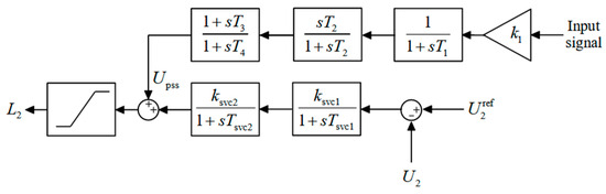
Figure 4. Block diagram of the static var compensator (SVC) controller.

The parameters $k_{\mathrm{s}\mathrm{v}\mathrm{c}1}$ and $k_{\mathrm{s}\mathrm{v}\mathrm{c}2}$ represent the loop gains, while $T_{\mathrm{s}\mathrm{v}\mathrm{c}1}$ and $T_{\mathrm{s}\mathrm{v}\mathrm{c}2}$ are the corresponding time constants of the SVC controller. The parameter $k_1$ denotes the gain, and $T_1$, $T_2$, $T_3$, and $T_4$ are the time constants of the control loop of the PSS.

5. Interactions in Offshore Power Systems

5.1. Characteristic of Interactions in Offshore Power System

Interactions can be described as the mutual influence of elements of the power system. In terms of slow-changing phenomena occurring in the power system, the types of interactions related to the influence of control systems presented in Table 1 can be specified. Interaction analysis in power systems provides insight into the dynamic relationships among individual control loops, subsystems, or system components. If not properly identified and mitigated, these interactions can lead to oscillations, reduced damping, degraded control performance, or even system instability.

Table 1. Characteristic frequencies for different types of interactions.

Type of Interaction	Frequency
Steady-state interactions	0 Hz
Electromechanical oscillation interactions	0–3/5 Hz
Control system coupling interactions	2–15
Sub-synchronous resonance interactions	2–50/60 Hz
Harmonic interactions, high-frequency resonance effects, and electromagnetic transient interactions	>15 Hz

Control can be implemented in either an open-loop or a closed-loop system. In an open-loop configuration, the control device does not receive feedback about the output signals but only information about the control objective and, possibly, external disturbances acting on the system. Such control is only feasible when the output signals can be accurately predicted based on the control input. In a closed-loop system, control signals are determined according to the measured output variables that define the control objective. This type of control depends on the system’s response and operates continuously until the desired objective is achieved.

Interaction analysis techniques can generally be classified as linear or nonlinear. The linear group includes sensitivity-based methods, such as eigenvalue and participation factor analysis [29,58,59], as well as interaction-matrix-based methods, including the RGA, DRGA, and GDRG [28,29,30,31,32,33,34,35,36,37,38,39,40,41,42,43,44,45,46,47,48,49,50,51,52,53,54,55,56,57,58,59,60,61]. In addition to these approaches, other methods have also been proposed in the literature that extend interaction beyond static measures such as the RGA or GDRG.

The Modal Decomposition Method [62,63,64,65], also known as Damping Torque Analysis, enables the evaluation of how individual controllers contribute to system oscillations. By transforming the system equations into a modal form, the method identifies the damping and synchronizing torque components associated with specific eigenvalues. It provides quantitative indicators—such as the Maximum Damping Influence—to evaluate how local control signals and controllers affect oscillatory modes and overall system stability. Although computationally more demanding, this approach offers deeper insight into modal interactions and is widely used to determine optimal controller placement and to design power system stabilizers and FACTS devices.

The Residue Method [29,63,64,66,67] focuses on analyzing the sensitivity of eigenvalues to variations in controller gains. It employs eigenvectors to evaluate how changes in controller parameters affect specific oscillatory modes. This approach enables the identification of controllers that have the greatest influence on system damping and interactions, and it is widely applied for tuning and optimal placement of control devices in large-scale power systems.

Methods based on Gramians [68,69] use controllability and observability Gramians of subsystems to measure the strength of input–output interactions. These methods show how system states can be controlled and observed. Calculated measures such as the Participation Matrix and the Hankel Interaction Index Array allow a systematic evaluation of coupling between system variables. They also help with the selection of optimal input–output pairings and the localization of control, similar to RGA-based approaches.

As a linear power system model was adopted for this study, linear interaction analysis methods—including the sensitivity method, the analysis of the transfer function, RGA, DRGA, and GDRG—are discussed in detail.

5.2. Sensitivity Method

Basic information about transient behaviour in a power system can be obtained from the eigenvalues of the state matrix $\mathbf{A}$, which are found by solving the characteristic Equation (10) [58]:

$$\mathrm{d}\mathrm{e}\mathrm{t}\left[\mathbf{A}-\lambda \mathbf{I}\right]=0$$

(10)

where $\lambda$ denotes the eigenvalue of the state matrix $\mathbf{A}$, and $\mathbf{I}$ is the identity matrix.

By solving Equation (10), the system eigenvalues ${\lambda }_i$ are obtained. Real eigenvalues correspond to non-oscillatory modes, whereas a pair of complex eigenvalues represents an oscillatory modes. For oscillatory eigenvalues of the form $\lambda =\sigma \mp \mathrm{j}\omega$, a positive real part $\sigma$ corresponds to a growing function over time, while a negative value indicates a decaying function. The damping ratio and oscillation frequency associated with such a mode are calculated using (11) and (12) [58]:

$$\xi ={\displaystyle \frac{-\sigma }{\sqrt{{\sigma }^2+{\omega }^2}}}$$

(11)

$$f_{\mathrm{o}\mathrm{s}\mathrm{c}}={\displaystyle \frac{\omega }{2\pi }}$$

(12)

Each eigenvalue ($j=\mathrm{1,2},\dots ,n$ where $n$ is the dimension of the state matrix) can be associated with a right and left eigenvector defined by (13) and (14) [70]:

$$\mathbf{A}{\mathbf{w}}_j={\lambda }_j{\mathbf{w}}_j\mathbf{A}\mathbf{w}$$

(13)

$${\mathbf{v}}_j^{\mathrm{T}}\mathbf{A}={\mathbf{v}}_j^{\mathrm{T}}{\lambda }_j$$

(14)

where ${\mathbf{w}}_j$ denotes the right eigenvector and ${\mathbf{v}}_j$ denotes the left eigenvector corresponding to the eigenvalue ${\lambda }_j$.

Sensitivity analysis makes it possible to determine which variations in system parameters cause shifts in the eigenvalues, particularly toward the imaginary axis. It also indicates which state variables have the greatest influence on a given eigenvalue ${\lambda }_j$. The sensitivity of eigenvalue ${\lambda }_j$ to parameter $p$ is given by (15):

$${\displaystyle \frac{{\partial \lambda }_j}{\partial p}}={\displaystyle \frac{\partial }{\partial p}}\left({\mathbf{v}}_j^{\mathrm{T}}A{\mathbf{w}}_j\right)={\mathbf{v}}_j^{\mathrm{T}}{\displaystyle \frac{\partial A}{\partial p}}{\mathbf{w}}_j$$

(15)

The degree to which the i-th state variable contributes to the j-th eigenvalue can be assessed using the participation factor defined in (16):

$$c_{ji}={\mathbf{v}}_{ji}{\mathbf{w}}_{ij}$$

(16)

5.3. Method of Magnitude Analysis of the Transfer Function G(s)

Based on linearized model given by (6) and (7), the matrix transfer function can be written as (17) [70]:

$$\mathbf{G}\left(s\right)={\mathbf{C}\left(s\mathbf{I}-\mathbf{A}\right)}^{-1}\mathbf{B}+\mathbf{D}$$

(17)

The elements of the matrix transfer function represent individual transfer functions that describe the relationships between specific input and output signals. In general form, the relationship between input and output signals can be expressed as (18):

$$\mathbf{Y}\left(s\right)=\left[\begin{array}{c}{Y}_1\left(s\right)\\ Y_2\left(s\right)\\ \dots \\ Y_m\left(s\right)\end{array}\right]=\left[\begin{array}{c}{G}_{11}\left(s\right)\\ G_{12}\left(s\right)\\ ⋮\\ G_{m1}\left(s\right)\end{array}\begin{array}{c}{G}_{21}\left(s\right)\\ G_{22}\left(s\right)\\ ⋮\\ G_{m1}\left(s\right)\end{array}\begin{array}{c}\dots \\ \dots \\ \\ \dots \end{array}\begin{array}{c}{G}_{1r}\left(s\right)\\ G_{2r}\left(s\right)\\ ⋮\\ G_{mr}\left(s\right)\end{array}\right]\left[\begin{array}{c}{U}_1\left(s\right)\\ U_2\left(s\right)\\ ⋮\\ U_r\left(s\right)\end{array}\right]$$

(18)

where $\mathbf{Y}\left(s\right)$—m-dimensional vector of Laplace transforms of output signals,$\mathbf{U}\left(s\right)$—r-dimensional vector of Laplace transforms of input signals (disturbances or control actions).

The transfer function between the j-th input and the i-th output is defined in (19):

$$G_{ij}\left(s\right)={\displaystyle \frac{∆Y_i\left(s\right)}{∆U_j\left(s\right)}} \mathrm{a}\mathrm{t} ∆U_k\left(s\right) \mathrm{f}\mathrm{o}\mathrm{r} k\ne j$$

(19)

where the matrix $G\left(s\right)$ has dimensions $m\times r$, ${∆Y}_i\left(s\right)$ is the Laplace transform of the output signal at the $i$-th node, and ${∆U}_j\left(s\right)$ is the Laplace transform of the input signal at the $j$-th node. Transfer characteristics derived from (17)–(19) are used to assess whether the selected controller input signals show a response within the considered frequency ranges and to what extent—for instance, through variations in amplitude or phase.

5.4. Relative Gain Array (RGA)

The RGA method is one of the simplest and most widely used techniques for analyzing control interactions in multivariable systems [28,29,65,71]. Originally introduced as a measure of control interaction [62], the method was later extended to the frequency domain. For a multivariable system, the RGA is defined as a matrix of relative gains, where each element represents the relationship between an input $u_j$ and an output $y_i$ in both open- and closed-loop conditions.

One of the most important properties of the RGA is that it depends solely on the system model, and not on the controller itself [62,63,64,66,67]. The RGA elements are calculated directly from the system transfer functions, without the need to compute eigenvalues. The relative gain between input $u_j$ and output $y_i$ is obtained from (20):

$${RGA}_{ij}={\left[{\left.{\displaystyle \frac{{\partial y}_i}{{\partial u}_j}}\right|}_{u_l=0, l\ne j}\right]\left[{\left.{\displaystyle \frac{{\partial y}_i}{{\partial u}_j}}\right|}_{y_l=0, l\ne j}\right]}^{-1}={\displaystyle \frac{g_{ij}\left(0\right)}{{\widehat{g}}_{ij}\left(0\right)}}$$

(20)

where $g_{ij}\left(0\right)$ denotes the gain between $u_j$ and $y_i$ when only the control signal $u_j$ is applied to the system, while ${\widehat{g}}_{ij}\left(0\right)$ represents the gain between $u_j$ and $y_i$ under ideal control conditions, in which all other output variables $y_i\left(l=1,\dots ,k;l\ne i\right)$ are maintained at their setpoint values. Therefore, for the output $y_i$ and the input $u_j$, the element ${RGA}_{ij}$ defines the effect of control on the gain between $u_i$ and $y_j$. Using the transfer function matrix defined in (17), the RGA matrix is obtained from (21):

$$\mathbf{R}\mathbf{G}\mathbf{A}\left[\mathbf{G}\left(0\right)\right]=\left[\mathbf{G}\left(0\right)\right]\otimes {\left[\mathbf{G}\left(0\right)\right]}^{\mathrm{T}}$$

(21)

where $\otimes$ denotes element-by-element multiplication, and the matrix transfer function is given by Equation (17).

Based on the RGA matrix, several interaction properties can be identified [65]:

• ${RGA}_{ij}=1$—no interaction between control loops; the pairing of input–output signals should follow the diagonal elements of the RGA matrix, i.e., $y_i-u_i$,
• ${RGA}_{ij}=0$—no interaction between control loops; the pairing of input–output signals should be off-diagonal, i.e., $y_i-u_j$ with $i\ne j$,
• ${RGA}_{ij}>1$—the gain increases when the control loops are closed, indicating the presence of interactions. The highest level of interaction occurs for large values of ${RGA}_{ij}$,
• ${0<RGA}_{ij}<1$—the gain decreases when the control loops are closed; interactions increase as ${RGA}_{ij}$ approaches unity,
• ${RGA}_{ij}<0$—the control loops are closed, and negative values of ${RGA}_{ij}$ indicate strong interaction; the larger the absolute value of ${RGA}_{ij}$, the stronger the coupling between control loops.

The RGA method is straightforward to implement and provides valuable data about potential control loop interactions. In addition to evaluating the degree of interaction, it can be used to identify suitable control input signals, determine optimal controller locations and detect oscillatory modes.

The coefficients ${RGA}_{ij}$ indicate how the open-loop gain $g_{ij}\left(0\right)$ changes when other control loops are closed. Recommended signal pairing rules are as follows:

• select signal pairs for which the RGA value is close to unity,
• avoid signal pairs with negative RGA values,
• avoid signal pairs for which the RGA values are significantly greater than one.

5.5. Dynamic Relative Gain Array (DRGA)

An important extension of the RGA method is the Dynamic Relative Gain Array (DRGA), which allows the analysis of input–output interactions over an arbitrary frequency range. The DRGA is defined in (22) [30]:

$$\wedge \left(G\left(\mathrm{j}\omega \right)\right)=G\left(\mathrm{j}\omega \right)\circ {\left({G\left(\mathrm{j}\omega \right)}^{-1}\right)}^{\mathrm{T}}$$

(22)

When analyzing a system, it is recommended to apply the DRGA to evaluate $\wedge \left(G\right)$ within the desired frequency range. The interpretation of system properties for the DRGA follows the same principles as for the RGA method.

5.6. Generalized Dynamic Relative Gain (GDRG)

The method that considers both the dynamics of the power system and the control system is the GDRG method [65,72]. The GDRG values are defined in (23):

$${GDRG}_{ii}={\displaystyle \frac{g_{ii}\left(s\right)}{h_{ii}^i\left(s\right)}}$$

(23)

where $g_{ii}\left(s\right)$ is the $(i,i)$ element of the open-loop transfer matrix $\mathbf{G}\left(s\right)$, while $h_{ii}^i\left(s\right)$ is the $(i,i)$ element of the closed-loop transfer matrix ${\mathbf{H}}^i\left(s\right)$ for the open-loop $u_i-y_i$, defined in (24):

$${\mathbf{H}}^i\left(s\right)={\left[\mathbf{I}-\mathbf{G}\left(s\right){\mathbf{G}}_C^i\left(s\right)\right]}^{-1}\mathbf{G}\left(s\right)=\left[h_{ij}^i\right]$$

(24)

where ${\mathbf{G}}_C^i\left(s\right)$ denotes a diagonal matrix of controller transfer functions, in which ${\mathbf{G}}_{Ci}^i\left(s\right)=0$ and $\mathbf{G}\left(s\right)$ represents the system transfer function matrix. As a measure of interaction within the control system, the GDRG index is calculated using (25):

$$N_{GDRG}\left(j\omega \right)={\sum }_{i=1}^k\left|{GDRG}_{ii}\left(j\omega \right)-1\right|$$

(25)

where $k$ denotes the number of individual controllers in an extended control system. From relationship (25), it can be concluded that a value of $N_{\mathrm{G}\mathrm{D}\mathrm{R}\mathrm{G}}\left(\mathrm{j}\omega \right)=0$ indicates the absence of interactions between control loops at a given frequency $\omega =2\mathrm{\pi }f$ [59].

In contrast to the RGA method, the GDRG can be applied to systems incorporating any type of controllers and is suitable for analyzing dynamic interactions among multifunctional controllers.

6. Interaction Analysis

The analysis was performed on the test system presented in Figure 2 and described in Section 4. The study considered variations in the loading of dynamic components: the synchronous generator (SG1) and the industrial load (VSD1), as well as changes in the study scenarios. In the next subsections, the results obtained using each selected method: eigenvalue analysis, amplitude–phase characteristics, RGA, DRGA and GDRG are presented.

6.1. Eigenvalue Analysis

As part of the preliminary studies, a small-signal analysis was performed. For the linear test system model, the state matrix A was derived, from which the eigenvalues, oscillation frequencies, and damping ratios were obtained. The participation factor analysis allows the identification of interactions—that is, the determination of the state variables influencing a given eigenvalue.

An example of participation factor analysis for Variant I, corresponding to selected eigenvalue ${\lambda }_{21}=-9.945+\mathrm{j}310.929$, is shown in Figure 5. The results indicate that the synchronous generator (SG1) makes the dominant contribution to this mode. The number in parentheses next to each participation value represent the number of the differential equations. The obtained results clearly indicate that, in this eigenvalue, the largest contribution comes from the synchronous generator (SG1). The numbers in parentheses next to each participation value correspond to the indices of the individual differential equations within the model of each system element.

Figure 5. An example distribution of participation factors for eigenvalue ${\lambda }_{21}$ in Variant I.

Table 2 presents the results for the frequency range associated with electromechanical oscillations under varying load conditions, while Table 3 corresponds to the range of electromagnetic oscillations.

Table 2. Results of eigenvalue analysis for changes in load for electromechanical oscillations.

Element	Eigenvalue	Frequency [Hz]	Damping [-]	Load
Synchronous Generator (Variant I)	−0.236 ± 5.263	0.838	0.045	25%
	−0.186 ± 5.360	0.853	0.035	50%
	−0.123 ± 5.507	0.877	0.022	75%
	−0.060 ± 5.674	0.903	0.010	100%
Synchronous Generator (Variant II)	−0.238 ± 5.279	0.840	0.045	25%
	−0.189 ± 5.374	0.855	0.035	50%
	−0.128 ± 5.517	0.878	0.023	75%
	−0.065 ± 5.681	0.904	0.011	100%
Synchronous Generator (Variant III)	−0.241 ± 5.281	0.840	0.046	25%
	−0.193 ± 5.375	0.856	0.036	50%
	−0.131 ± 5.518	0.878	0.024	75%
	−0.069 ± 5.680	0.904	0.012	100%

Table 3. Results of eigenvalue analysis for changes in load for electromagnetic oscillations.

Element	Eigenvalue	Frequency [Hz]	Damping [-]	Load
Synchronous Generator (Variant I)	−17.533 ± 317.279	50.496	0.055	25%
	−17.539 ± 317.281	50.497	0.055	50%
	−17.542 ± 317.283	50.497	0.055	75%
	−17.546 ± 317.284	50.497	0.055	100%
Synchronous Generator (Variant II)	−17.480 ± 317.403	50.516	0.055	25%
	−17.486 ± 317.406	50.517	0.055	50%
	−17.490 ± 317.408	50.517	0.055	75%
	−17.493 ± 317.408	50.517	0.055	100%
Synchronous Generator (Variant III)	−17.363 ± 317.548	50.539	0.055	25%
	−17.369 ± 317.551	50.540	0.055	50%
	−17.373 ± 317.552	50.540	0.055	75%
	−17.376 ± 317.553	50.540	0.055	100%

6.2. Amplitude–Phase Characteristics Analysis

The amplitude–phase characteristics were developed for two input–output pairs (Table 4) within two frequency ranges: the electromechanical oscillation range (approximately 0.2–2.5 Hz) and the range of oscillations near the fundamental frequency (approximately 47–53 Hz). The analysis was carried out under varying load conditions.

Table 4. List of input–output pairs for amplitude–phase characteristic analysis.

Input–Output	Description
$U_{\mathrm{p}\mathrm{s}\mathrm{s}\left(\mathrm{s}\mathrm{g}1\right)}-P_{\mathrm{s}\mathrm{g}1}$	➢ input signal of the PSS of the synchronous generator ➢ synchronous generator active power
$U_{\mathrm{p}\mathrm{s}\mathrm{s}\left(\mathrm{s}\mathrm{g}1\right)}-q_{\mathrm{s}\mathrm{g}1}$	➢ input signal of the PSS of the synchronous generator ➢ signal of the synchronous generator voltage components

For the purpose of quantifying the interactions, three measures were defined: the maximum amplitude within the considered frequency ranges (26), the corresponding frequency at which this maximum occurs (27), and the associated phase value (28).

$$A_1=A_{\mathrm{m}\mathrm{a}\mathrm{x}} for f=\left[0÷3 \mathrm{H}\mathrm{z}\right] A_2=A_{\mathrm{m}\mathrm{a}\mathrm{x}} for f=\left[40÷60 \mathrm{H}\mathrm{z}\right]$$

(26)

$$f_1=f\left(A_1\right) f_2=f\left(A_2\right)$$

(27)

$${\phi }_1=\phi \left(A_1\right) {\phi }_2=\phi \left(A_2\right)$$

(28)

Table 5 and Table 6 present the results for Variant I, II, and III for the measures defined by Equations (26)–(28). Figure 6 and Figure 7 present the amplitude plots and Figure 8 and Figure 9 the phase plots for pair $U_{\mathrm{p}\mathrm{s}\mathrm{s}\left(\mathrm{s}\mathrm{g}1\right)}-P_{\mathrm{s}\mathrm{g}1}$ and $U_{\mathrm{p}\mathrm{s}\mathrm{s}\left(\mathrm{s}\mathrm{g}1\right)}-q_{\mathrm{s}\mathrm{g}1}$ for Variant I.

Table 5. Selected values from the amplitude–phase plots for the pair $U_{\mathrm{p}\mathrm{s}\mathrm{s}\left(\mathrm{s}\mathrm{g}1\right)}-P_{\mathrm{s}\mathrm{g}1}$.

Variant	0.5–3 Hz			47–53 Hz			Load
	${\mathit{A}}_1$ [abs]	${\mathit{f}}_1$ [Hz]	${\mathit{\phi }}_1$ [°]	${\mathit{A}}_2$ [abs]	${\mathit{f}}_2$ [Hz]	${\mathit{\phi }}_2$ [°]
I	9.089	0.839	79.963	0.042	49.510	−232.629	25%
	20.956	0.854	80.275	0.070	40.000	−172.030	50%
	43.768	0.877	81.081	0.102	40.000	−171.347	75%
	109.918	0.903	82.016	0.135	40.000	−170.730	100%
II	3.690	0.837	80.848	0.039	49.474	−238.269	25%
	20.220	0.856	80.476	0.071	40.000	−171.986	50%
	41.485	0.878	81.239	0.102	40.000	−171.306	75%
	99.347	0.904	82.131	0.135	40.000	−170.690	100%
III	8.713	0.841	80.236	0.044	49.447	−231.277	25%
	19.821	0.856	80.515	0.071	40.000	−171.967	50%
	40.307	0.878	81.271	0.102	40.000	−171.287	75%
	94.162	0.904	82.155	0.135	40.000	−170.671	100%

Table 6. Selected values from the amplitude–phase characteristics for the pair $U_{\mathrm{p}\mathrm{s}\mathrm{s}\left(\mathrm{s}\mathrm{g}1\right)}-q_{\mathrm{s}\mathrm{g}1}$.

Variant	0.5–3 Hz			47–53 Hz			Load
	${\mathit{A}}_1$ [abs]	${\mathit{f}}_1$ [Hz]	${\mathit{\phi }}_1$ [°]	${\mathit{A}}_2$ [abs]	${\mathit{f}}_2$ [Hz]	${\mathit{\phi }}_2$ [°]
I	0.281	0.839	1614.300	0.003	47.971	1256.201	25%
	0.898	0.854	1614.800	0.002	53.288	806.580	50%
	1.722	0.877	1615.800	0.002	53.287	795.829	75%
	3.459	0.903	1616.900	0.002	53.286	789.977	100%
II	0.019	0.838	1614.900	0.003	47.972	1261.570	25%
	0.726	0.856	1614.900	0.003	47.972	1242.520	50%
	1.401	0.878	1615.800	0.003	47.972	1233.770	75%
	2.695	0.904	1616.900	0.003	47.972	1228.440	100%
III	0.157	0.841	1614.400	0.003	47.972	1253.180	25%
	0.612	0.856	1614.800	0.003	47.972	1241.920	50%
	1.189	0.878	1615.700	0.003	47.972	1233.430	75%
	2.221	0.904	1616.700	0.003	47.972	1228.270	100%

Figure 6. Amplitude plots for the pair $U_{\mathrm{p}\mathrm{s}\mathrm{s}\left(\mathrm{s}\mathrm{g}1\right)}-P_{\mathrm{s}\mathrm{g}1}$ in the frequency range of 0–3 Hz and 47–53 Hz (Variant I)—load variation.

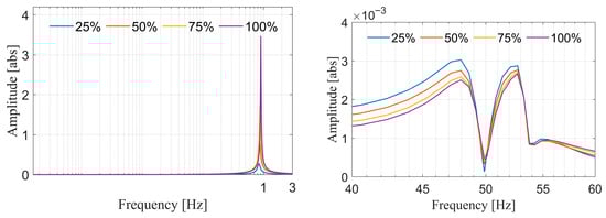
Figure 7. Amplitude plots for the pair $U_{\mathrm{p}\mathrm{s}\mathrm{s}\left(\mathrm{s}\mathrm{g}1\right)}-q_{\mathrm{s}\mathrm{g}1}$ in the frequency range of 0–3 Hz and 47–53 Hz (Variant I)—load variation.

Figure 8. Phase plots for the pair $U_{\mathrm{p}\mathrm{s}\mathrm{s}\left(\mathrm{s}\mathrm{g}1\right)}-P_{\mathrm{s}\mathrm{g}1}$ in the frequency range of 0–3 Hz and 47–53 Hz (Variant I)—load variation.

Figure 9. Phase plots for the pair $U_{\mathrm{p}\mathrm{s}\mathrm{s}\left(\mathrm{s}\mathrm{g}1\right)}-q_{\mathrm{s}\mathrm{g}1}$ in the frequency range of 0–3 Hz and 47–53 Hz (Variant I)—load variation.

6.3. Relative Gain Array (RGA) Analysis

In the RGA analysis of the test system, the RGA matrix was obtained using Equation (21). When two signal pairs are considered, the resulting matrix has dimensions of 2 × 2. The results are illustrated by the variation in the values in the two columns of the first row of the RGA matrix, namely RGA(1,1) and RGA(1,2). The analysis was performed for the signals listed in Table 7 under varying load conditions, with the corresponding RGA results presented in Table 8.

Table 7. List of input–output pairs for RGA analysis.

Signals		Description
Input:	$U_{\mathrm{p}\mathrm{s}\mathrm{s}}$ $U_{\mathrm{p}\mathrm{s}\mathrm{s}\left(\mathrm{s}\mathrm{g}1\right)}$	➢ input signal of the SVC controller ➢ input signal of the synchronous generator controller
Output:	$P_{\mathrm{s}\mathrm{g}1}$ $q_{\mathrm{s}\mathrm{g}1}$	➢ synchronous generator active power ➢ signal of the synchronous generator voltage components

Table 8. Results of interaction analysis using the RGA method for the pair $P_{\mathrm{s}\mathrm{g}1}- q_{\mathrm{s}\mathrm{g}1}$.

Variant	I				II				III
Load	25%	50%	75%	100%	25%	50%	75%	100%	25%	50%	75%	100%
RGA (1,1)	0.0002	0.0003	0.0004	0.0004	0.0001	0.0003	0.0004	0.0004	0.0002	0.0003	0.0004	0.0004
RGA (1,2)	0.9998	0.9997	0.9996	0.9996	0.9999	0.9997	0.9997	0.9996	0.9999	0.9997	0.9996	0.9996

6.4. Dynamic Relative Gain Array (DRGA) Analysis

The Dynamic Relative Gain Array (DRGA) characteristics were obtained within two frequency ranges: the electromechanical oscillation range (approximately 0.2–2.5 Hz) and the range of oscillations near the fundamental frequency (approximately 47–53 Hz). The resulting DRGA characteristics, particularly at higher frequencies, were found to be significantly distorted. In this study, the DRGA method was enhanced by introducing an additional digital filtering stage. For this purpose, a hybrid filtering approach was applied, combining Finite Impulse Response (FIR) and Infinite Impulse Response (IIR) filters. The filtering process, illustrated in Figure 10, modifies the input signal by multiplying its transform with the transfer function of the combined filter, as expressed in (29) [73]:

$$Y\left(z\right)={\displaystyle \frac{b\left(1\right)+b\left(2\right)z^{-1}+\cdots +b\left(n_b+1\right)z^{-n_b}}{1+a\left(2\right)z^{-1}+\cdots +a\left(n_a+1\right)z^{-n_a}}}X\left(z\right)$$

(29)

where $b$, $a$ are the coefficients of the polynomials, $X\left(z\right)$ is the transform of the input signal $x$, $Y\left(z\right)$ is the transform of the output signal $y$, $n_a$ is the order of the feedback filter, and $n_b$ is the order of the feedforward filter.

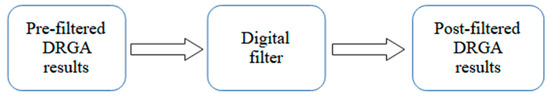
Figure 10. Block diagram of the digital filtering process for DRGA.

The proposed filtering stage effectively reduces high-frequency distortions and improves the accuracy of the DRGA-based interaction assessment without altering the essential dynamic characteristics of the system. A comparison of the characteristic before and after applying the proposed digital filtering process is presented in Figure 11.

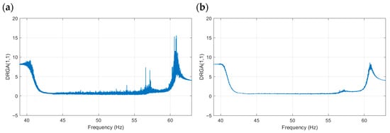
Figure 11. Example of a DRGA characteristic after filtering (a) pre-filtered DRGA results, (b) post-filtered DRGA Results.

The analysis was performed for the same signals as in RGA method. The results for Variant I are presented in Figure 12, Variant II in Figure 13 and Variant III in Figure 14.

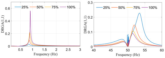
Figure 12. Results of DRGA values for the pair $P_{\mathrm{s}\mathrm{g}1}- q_{\mathrm{s}\mathrm{g}1}$ (Variant I).

Figure 13. Results of DRGA values for the pair $P_{\mathrm{s}\mathrm{g}1}- q_{\mathrm{s}\mathrm{g}1}$ (Variant II).

Figure 14. Results of DRGA values for the pair $P_{\mathrm{s}\mathrm{g}1}- q_{\mathrm{s}\mathrm{g}1}$ (Variant III).

For Variant I (Figure 12), the test system exhibits electromechanical resonance around 1 Hz and an electromagnetic resonance near 50 Hz. In the case of Variant II (Figure 13), the amplitudes of the resonant peaks at both frequencies are reduced compared to Variant I. For Variant III (Figure 14), the characteristic resonance peaks observed in the previous variants are largely suppressed and the high-frequency response becomes more dispersed. Although the 25% loading case exhibits a slightly higher local peak below 50 Hz, this behaviour is consistent with the reduced inherent damping of the lightly loaded synchronous generator. Overall, the expanded power system structure can lead reduced sensitivity to dynamic interactions.

6.5. Generalized Dynamic Relative Gain (GDRG) Analysis

The RGA method is simple to apply; however, it does not consider the controller structure and is therefore typically used in the early phase of interaction studies. Further analyses following the RGA assessment should consider the structure and parameters of the applied controllers. In the case of the GDRG method, the analyzed components were the power system stabilizer controllers within the SVC and synchronous generator systems. The signal pairs were selected based on the DRGA analysis, where interactions within the range of electromechanical oscillations were observed. Accordingly, the input signals to the control systems of the power system stabilizer within the SVC and the synchronous generator were $P_{\mathrm{s}\mathrm{g}1}- q_{\mathrm{s}\mathrm{g}1}$. The results of the GDRG coefficient for frequency both frequencies are presented in Figure 15 for Variant I, Figure 16 for Variant II, and Figure 17 for Variant III.

Figure 15. Results of GDRG values for the pair $P_{\mathrm{s}\mathrm{g}1}- q_{\mathrm{s}\mathrm{g}1}$—Variant I.

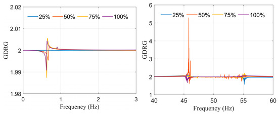
Figure 16. Results of GDRG values for the pair $P_{\mathrm{s}\mathrm{g}1}- q_{\mathrm{s}\mathrm{g}1}$—Variant II.

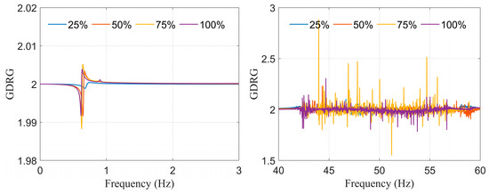
Figure 17. Results of GDRG values for the pair $P_{\mathrm{s}\mathrm{g}1}- q_{\mathrm{s}\mathrm{g}1}$—Variant III.

6.6. Interaction Analysis Discussion

The proposed test model was evaluated under varying loading conditions (25–100%) of selected elements and across three configuration variants. The analysis employed several complementary methods, including sensitivity analysis, amplitude–phase plots, the RGA, DRGA, and GDRG methods. Table 9 presents the comparison for different interaction analysis methods used in this study.

Table 9. Comparison of different interaction analysis methods.

Method	Advantages	Disadvantages
Eigenvalues	Relatively easy to implement in a simulation tool (built-in function), assuming that the linearized model is available. This method allows for accurate analysis of the test model.	A large number of output data for highly complex models; lack of information identifying specific eigenvalues.
Participation Factors	Essential when analyzing eigenvalues, providing complementary information without which the study would be difficult to perform.	More difficult to implement—in the considered simulation tool there is no built-in function available.
Frequency Response Characteristics	Useful for signal analysis, providing relatively extensive information over any frequency range. Enables preliminary signal verification before applying other methods.	Fairly laborious implementation—requires manual selection of input–output pairs. Relatively long computation time.
RGA	Useful in preliminary analysis of signals selected for the control system; easy to implement and computationally simple. Not sufficient as a standalone interaction analysis method.	Limited matrix size (recommended 2 × 2), does not include the controller model, and analyses only a single frequency point.
DRGA	Any frequency range can be analyzed; provides more information compared to RGA.	Difficult to implement; longer computation time.

The first analysis consisted in performing a sensitivity study using eigenvalue analysis. In the case of electromechanical oscillations, it can be observed that loading the synchronous generator causes changes in both the oscillation frequency and the damping ratio. The frequencies in this range increase with loading, while the damping decreases. These results were confirmed for all variants of the power system configuration. The change in the load of dynamic system components resulted in variations in the frequency and damping associated with high-power consumption, whereas it had no significant effect on the eigenvalues related to the synchronous generator.

The next method applied to the interaction analysis was the frequency response (amplitude–phase) characteristic. It can be observed that for the selected analyzed signals, with a change in load and within the range of electromechanical oscillations, a significant increase in amplitude and a frequency shift occurred. Moreover, the change in load had no noticeable impact on the range of electromagnetic oscillations. The amplitude of the base system in the range of electromechanical oscillations was 3.459 at a frequency of 0.903 Hz (Variant I), 2.695 at 0.904 Hz (Variant II), and 2.221 at 0.904 Hz (Variant III). For the electromechanical oscillations, no significant amplitude changes were observed when varying the system configuration for the analyzed factors.

Subsequently, the interaction analyses were performed using the RGA method and its extension, the DRGA. For the selected signal pair, the change in load did not cause any change in the RGA values, and the obtained results did not indicate the presence of interactions. The same conclusions were observed regardless of the power system configuration variant.

In the case of DRGA, for Variant I (Figure 12) the test system exhibits electromechanical resonance around 1 Hz and electromagnetic resonance near 50 Hz. The DRGA values within the electromechanical range tend to increase with loading, indicating stronger interactions at higher load levels. For Variant II (Figure 13), the amplitudes of the resonant peaks at both frequencies are reduced compared to Variant I, which shows that the additional network elements provide effective damping. Although the overall trend of increasing DRGA values with load remains visible, the absolute amplitudes in both the electromechanical and electromagnetic ranges are lower. More significant differences appear in the electromagnetic oscillation range. Compared with Variant I, Variant II exhibits additional frequency components introduced by the expanded network structure. The DRGA values in this range still point to the presence of interactions, but their amplitudes are smaller and less pronounced. For Variant III (Figure 14), the characteristic resonance peaks observed in the previous variants are largely suppressed, and the high-frequency response becomes more dispersed. Although the 25% loading case exhibits a slightly higher local peak below 50 Hz, this behaviour is consistent with the reduced inherent damping of the lightly loaded synchronous. In both the electromechanical and electromagnetic frequency ranges, Variant III shows a further reduction in DRGA values, accompanied by frequency shifts. Overall, the expanded power system structure leads to significantly reduced sensitivity to dynamic interactions.

In the case of GDRG, for Variant I (Figure 15) the results show clear resonance values in both analyzed frequency ranges. In the electromechanical range (0–3 Hz), the GDRG values remain close to 2, with a noticeable peak around 0.9 Hz that can reflects the response of the synchronous generator. In the electromagnetic range (40–60 Hz), peaks occur around 50 Hz, indicating a strong high-frequency interaction typical for the Variant I with fewer system elements. For Variant II (Figure 16), the overall GDRG levels in both frequency ranges are lower than in Variant I. The peak around 0.9 Hz is still present but less distinct. In the electromagnetic range, the dominant resonance near 50 Hz becomes substantially weaker. There are also additional small oscillatory components introduced by the expanded network structure. These results suggest that incorporating more components leads to a wider distribution of values and reduces GDRG magnitude. For Variant III (Figure 17), the characteristic peaks observed in the earlier variants are largely suppressed. In the low-frequency range, the GDRG values remain close to 2 with minimal variation. In the high-frequency range, the response no longer features a single dominant peak; instead, it becomes more irregular and dispersed, with several small fluctuations. Overall, Variant III demonstrates the more complex interaction characteristics.

7. Summary

This study presents an interaction analysis of an offshore power system comprising both renewable and conventional energy sources, as well as industrial loads (static loads and a variable-speed drive). An analysis of the related work shows that there has been a gap in research on interactions in offshore power systems. Additionally, a literature review revealed a lack of dedicated software for performing interaction analyses. Therefore, the authors of this paper developed their own models and developed a suitable simulation tool to perform interaction analyses.

For the purpose of interaction analysis, a linearized model of the offshore power system was developed, and several linear interaction analysis methods were implemented, including the sensitivity method, transfer function analysis, RGA, DRGA, and GDRG. The developed model and applied methods allow the investigation of interactions within the ranges of electromechanical oscillations and sub-synchronous resonance phenomena. The results presented in this paper demonstrate that the use of a single interaction analysis method does not provide a complete understanding of the phenomena occurring in the system.

The findings from the interaction analyses conducted using the selected methods can be summarized as follows:

• The transfer function analysis method and the RGA are suitable for studying the properties of controller input signals but do not account for the influence of controller design. Therefore, these methods are most appropriate during the preliminary stage of analysis.
• To obtain a more comprehensive assessment, it is necessary to apply methods such as the DRGA and GDRG, which consider the dynamic characteristics of the designed controllers. Due to the specific nature of offshore power systems, the direct implementation of interaction analysis methods may face difficulties. This has been illustrated in the paper using the example of the DRGA method.
• Direct application of the DRGA led to highly distorted characteristics that prevented proper interaction assessment. To address this, a modified version of the DRGA was proposed, incorporating an additional filtering stage combining Finite Impulse Response (FIR) and Infinite Impulse Response (IIR) filters. The proposed modification effectively reduced distortions and enabled reliable interaction analysis and system property evaluation.
• The results showed that interactions in offshore power systems are influenced by factors such as system configuration and operating point. Therefore, multivariant interaction analyses are required to properly evaluate system behaviour under different operating conditions.

Another important contribution of this study is the comparative summary of the advantages and limitations of various interaction analysis methods. The presented comparison may serve as a practical reference for researchers investigating control interactions in power systems.

Future research on interaction analysis in offshore power systems should focus on developing a systematic methodology for interaction studies, testing a wider spectrum of factors affecting different types of interactions, and optimizing control system parameters with respect to control-loop interactions. It also seems appropriate to extend research to analyses employing non-linear interaction methods.

References

- Minister Kurtyka on RES in the Polish Energy Mix—Ministry of Climate and Environment—Gov.pl Website. Available online: https://www.gov.pl/web/climate/minister-kurtyka-on-res-in-the-polish-energy-mix (accessed on 15 August 2025).
- Nguyen, P.Q.P.; Dong, V.H. Ocean Energy—A Clean Energy Source. Eur. J. Eng. Res. Sci. 2019, 4, 5–11. [Google Scholar] [CrossRef]
- Robak, S.; Raczkowski, R.; Piekarz, M. Development of the Wind Generation Sector and Its Effect on the Grid Operation—The Case of Poland. Energies 2023, 16, 6805. [Google Scholar] [CrossRef]
- Pruski, P.; Paszek, S. Analiza modalna przebiegów zakłóceniowych mocy chwilowej w krajowym systemie elektroenergetycznym. Elektryka 2011, 4, 81–96. [Google Scholar]
- Mithulananthan, N.; Cañizares, C.A.; Reeve, J. Tuning, Performance and Interactions of PSS and FACTS Controllers. Proc. IEEE Power Eng. Soc. Transm. Distrib. Conf. 2002, 2, 981–987. [Google Scholar] [CrossRef]
- GWEC. Global Offshore Wind Report 2025. Offshore Capacity Reached 83 GW by end-2024 with 8 GW Added. Available online: https://www.gwec.net/gwec-news/offshore-wind-installed-capacity-reaches-83-gw-as-new-report-finds-2024-a-record-year-for-construction-and-auctions (accessed on 7 August 2025).
- WindTech-International. Offshore Wind Additions in 2023 ~10.8 GW; Global Capacity 64.3 GW. 2025. Available online: https://www.mercomindia.com/global-offshore-wind-capacity-rises (accessed on 9 August 2025).
- GWEC. Global Wind Report 2025. Record 117 GW of New Wind Capacity in 2024; Offshore Share ~8 GW. Available online: https://renewablesnow.com/news/global-wind-installations-reach-record-117-gw-in-2024-gwec-1274126/ (accessed on 10 August 2025).
- GWEC. Forecast: Annual Offshore Installations to Rise from 16 GW in 2025 to 34 GW in 2030. 2025. Available online: https://www.gwec.net/gwec-news/wind-industry-installs-record-capacity-in-2024-despite-policy-instability (accessed on 10 August 2025).
- BloombergNEF; IEA. Offshore Capacity Projections: 218–258 GW by 2030. 2024. Available online: https://ember-energy.org/latest-insights/offshore-wind-targets-underpin-acceleration-to-2030-and-beyond/ (accessed on 10 August 2025).
- IRENA; ERM. Required Offshore Capacity for 1.5 °C Pathway: 494 GW by 2030, >2400 GW by 2050. 2024. Available online: https://www.erm.com/about/news/report-finds-most-countries-expected-to-miss-net-zero-offshore-wind-targets/ (accessed on 10 August 2025).
- Xie, X.; Shair, J.; Beerten, J.; Fan, L.; Gomis-Bellmunt, O.; Vorobev, P.; Preece, R.; Shah, S.; Wang, X.; Wang, Y.; et al. Guest Editorial: Control Interactions in Power Electronic Converter-Dominated Power Systems. Int. J. Electr. Power Energy Syst. 2024, 155, 109553. [Google Scholar] [CrossRef]
- Khaki-Sedigh, A.; Moaveni, B. Control Configuration Selection for Multivariable Plants; Lecture Notes in Control and Information Sciences; Springer: Berlin/Heidelberg, Germany, 2009. [Google Scholar] [CrossRef]
- Upadhyaya, S.; Veerachary, M. Interaction Quantification in Multi-Input Multi-Output Integrated DC-DC Converters. In Proceedings of the 2021 IEEE 4th International Conference on Computing, Power and Communication Technologies (GUCON 2021), Kuala Lumpur, Malaysia, 24–26 September 2021. [Google Scholar] [CrossRef]
- Robak, S.; Machowski, J.; Gryszpanowicz, K. Contingency Selection for Power System Stability Analysis. In Proceedings of the 18th International Scientific Conference on Electric Power Engineering (EPE), Kouty nad Desnou, Czech Republic, 17–19 May 2017; Volume 1, pp. 1–5. [Google Scholar]
- IRENA. Global Renewables Outlook 2020—Summary; International Renewable Energy Agency: Abu Dhabi, United Arab Emirates, 2020; Available online: https://www.irena.org/-/media/Files/IRENA/Agency/Publiction/2020/Apr/IRENA_GRO_Summary_2020.pdf (accessed on 4 December 2025).
- Cai, L.J.; Erlich, I. Simultaneous Coordinated Tuning of PSS and FACTS Damping Controllers in Large Power Systems. IEEE Trans. Power Syst. 2005, 20, 294–300. [Google Scholar] [CrossRef]
- Karawita, C.; Annakkage, U.D. HVDC-Generator-Turbine Torsional Interaction Studies Using a Linearized Model with Dynamic Network Representation. Change 2009, 10, 4. [Google Scholar]
- Xiao, H.; Li, Y. Multi-Infeed Voltage Interaction Factor: A Unified Measure of Inter-Inverter Interactions in Hybrid Multi-Infeed HVDC Systems. IEEE Trans. Power Deliv. 2020, 35, 2040–2048. [Google Scholar] [CrossRef]
- Bi, J.; Sun, H.; Guo, J.; Xu, S.; Yi, J.; Song, R. Influence of Dynamic Interaction Between Multiple DFIGs on Low-Frequency Oscillation of Power System. In Proceedings of the 2019 IEEE Power & Energy Society General Meeting (PESGM), Atlanta, GA, USA, 4–8 August 2019. [Google Scholar] [CrossRef]
- Li, P.; Wang, J.; Xiong, L.; Ma, M. Robust Nonlinear Controller Design for Damping of Sub-Synchronous Control Interaction in DFIG-Based Wind Farms. IEEE Access 2019, 7, 16626–16637. [Google Scholar] [CrossRef]
- Ye, J.; Li, S.; Feng, P.; Wang, X. Passive Control Strategy to Mitigate Sub-Synchronous Control Interaction of DFIG-Based Integrated Power Systems. In Proceedings of the 2023 International Conference on Power System Technology (PowerCon 2023), Jinan, China, 21–22 September 2023. [Google Scholar] [CrossRef]
- Tao, G.; Wang, Y.; Wu, Y.; Chen, Y. Subsynchronous Interaction Analysis of PMSG-Based Wind Farm with AC Networks. In Proceedings of the 22nd International Conference on Electrical Machines and Systems (ICEMS 2019), Harbin, China, 11–14 August 2019. [Google Scholar] [CrossRef]
- Li, P.; Wang, J.; Xiong, L.; Huang, S.; Ma, M.; Wang, Z. Energy-Shaping Controller for DFIG-Based Wind Farm to Mitigate Subsynchronous Control Interaction. IEEE Trans. Power Syst. 2021, 36, 2975–2991. [Google Scholar] [CrossRef]
- Liu, Y.; Huang, B.; Sun, H.; Zhang, Y.; Han, Y.; Yu, Y. Optimization of Control Parameters for PMSG-Based Wind Farm and SVG Considering Subsynchronous Interaction. In Proceedings of the 8th Renewable Power Generation Conference (RPG 2019), Shanghai, China, 24–25 October 2019; p. CP764. [Google Scholar] [CrossRef]
- Li, W.; Zheng, W.; Chen, Y. Stability and Interaction Analysis of PMSG-Based Wind Farms Connected with LCC-HVDC. In Proceedings of the 2023 Chinese Control and Decision Conference (CCDC 2023), Yichang, China, 20–22 May 2023; pp. 1361–1367. [Google Scholar] [CrossRef]
- Sun, W.; Wang, Q.; Cai, H.; Zhang, W.; Qi, W.; Xu, S.; Zhao, E. Interaction Between PMSG-Based Wind Farm and VSC-HVDC System in ACC Timescale. In Proceedings of the 2022 IEEE 5th International Electrical and Energy Conference (CIEEC 2022), Nangjing, China, 27–29 May 2022; pp. 2197–2201. [Google Scholar] [CrossRef]
- Bristol, E.H. On a New Measure of Interaction for Multivariable Process Control. IEEE Trans. Autom. Control 1966, 11, 133–134. [Google Scholar] [CrossRef]
- Messina, A.R.; Begovich, O.; López, J.H.; Reyes, E.N. Design of Multiple FACTS Controllers for Damping Inter-Area Oscillations: A Decentralised Control Approach. Int. J. Electr. Power Energy Syst. 2004, 26, 19–29. [Google Scholar] [CrossRef]
- Kinnaert, M. Interaction Measures and Pairing of Controlled and Manipulated Variables for Multiple-Input-Multiple-Output Systems: A Survey. Journal A 1995, 36, 15–23. [Google Scholar]
- Agbemuko, A.J. Dynamic Modelling and Interaction Analysis of Multi-terminal HVDC Systems. Int. J. Electr. Power Energy Syst. 2019, 113, 874–887. [Google Scholar] [CrossRef]
- Shi, J.; Chen, W.; Wei, Z.; Pei, X.; Sun, X. Quantitative Analysis of the Interactive Influence for Harmonic Emission in Wind Farms. Front. Energy Res. 2022, 9, 820963. [Google Scholar] [CrossRef]
- Cheah Mane, M. Sub-Synchronous Interactions in Wind Integrated Power Systems; Wiley: Hoboken, NJ, USA, 2023. [Google Scholar]
- Mugambi, G.R.; Darii, N.; Khazraj, H.; Romano, O.S.; Raducu, A.G.; Sharma, R.; Cutululis, N.A. Methodologies for Offshore Wind Power Plants Stability Analysis. arXiv 2024, arXiv:2410.13521v1. [Google Scholar] [CrossRef]
- Jacobson, M.Z.; Delucchi, M.A.; Cameron, M.A.; Mathiesen, B.V.; Østergaard, P.A.; Boschetti, L.; Cisilino, A.; Fajardy, M.; Briner, G.; Long, G.; et al. 100% Clean and Renewable Wind, Water, and Sunlight (WWS) All-Sector Energy Roadmaps for 139 Countries of the World. Energy Policy 2021, 149, 112111. Available online: https://web.stanford.edu/group/efmh/jacobson/Articles/I/CountriesWWS.pdf (accessed on 4 December 2025).
- European Parliamentary Research Service (EPRS). Japan’s 2050 Goal: A Carbon-Neutral Society; European Parliament: Brussels, Belgium, 2021. Available online: https://www.europarl.europa.eu/RegData/etudes/BRIE/2021/698023/EPRS_BRI(2021)698023_EN.pdf (accessed on 4 December 2025).
- Banet, C.; Willems, B. Scaling up Offshore Wind Energy in Europe; CERRE: Brussels, Belgium, 2023; Available online: https://cerre.eu/wp-content/uploads/2023/10/CERRE-REPORT-OFFSHOREWINDINEUROPE.OCT23-2-1.pdf (accessed on 4 December 2025).
- Icaza-Alvarez, D.; Galan-Hernandez, N.D.; Orozco-Guillen, E.E.; Jurado, F. Smart Energy Planning in the Midst of a Technological and Political Change towards a 100% Renewable System in Mexico by 2050. Energies 2023, 16, 7121. [Google Scholar] [CrossRef]
- Icaza-Alvarez, D.; Jurado, F.; Tostado-Véliz, M. Smart energy transition with the inclusion of floating wind energy in existing hydroelectric reservoirs with a view to 2050. Ecuadorian case study. Energy Rep. 2023, 10, 2804–2816. [Google Scholar] [CrossRef]
- Department of Mineral Resources and Energy (DMRE). Comments and Responses on the Draft Integrated Resource Plan (IRP) 2023; DMRE: Pretoria, South Africa, 2024. Available online: https://www.dmre.gov.za/Portals/0/Energy%20Resources/IRP/IRP%202025/Comments-and-Responses-on-the-Draft-IRP.pdf?ver=SYi03wt4df8ObzUMUkU8Ng%3D%3D (accessed on 4 December 2025).
- Kakoulaki, G.; Gonzalez-Sanchez, R.; Gracia-Amillo, A.; Szabó, S.; Farinosi, F.; De Felice, L.; Bisselink, B.; Seliger, R.; De Felice, M.; Kougias, I.; et al. Benefits of Pairing Floating Solar Photovoltaics with Hydropower Reservoirs in Europe. Renew. Sustain. Energy Rev. 2023, 171, 112989. [Google Scholar] [CrossRef]
- Vidović, V.; Krajačić, G.; Matak, N.; Stunjek, G.; Mimica, M. Review of the Potentials for Implementation of Floating Solar Panels on Lakes and Water Reservoirs. Renew. Sustain. Energy Rev. 2023, 178, 113237. [Google Scholar] [CrossRef]
- Robak, S.; Piekarz, M. Problematyka stabilności kątowej morskich systemów elektroenergetycznych. Przegląd Elektrotech. 2015, 91, 278–283. [Google Scholar] [CrossRef][Green Version]
- Robak, S. Sources of Uncertainty in Power System Analysis. Przegląd Elektrotech. 2008, 84, 54–57. [Google Scholar]
- Equinor Industriminne. Powering Johan Sverdrup from Shore. Available online: https://www.equinor.com/news/archive/2018-10-09-johan-sverdrup-powered-shore (accessed on 10 September 2025).
- Thema Consulting/OffshoreNorge. Electrification of the Oil and Gas Sector–Thema Report 2022–2023. OffshoreNorge, January 2023. Available online: https://www.offshorenorge.no/contentassets/97cb69dec47d4ecbaff23c16af5ce50c/thema-report_2022-23_electrification-of-the-oil-and-gas-sector-endelig-1.pdf (accessed on 16 September 2025).
- Precise Consultants. Dutch subsidy Enables World’s First Offshore Green Hydrogen Project. Precise Consultants. Available online: https://www.preciseconsultants.com/news/dutch-subsidy-enables-world-s-first-offshore-green-hydrogen-project/ (accessed on 4 October 2025).
- OEDigital. Lhyfe Meets Its Green Hydrogen Objectives with First Offshore Demonstrator; OEDigital: Mildura, Australia, 2024; Available online: https://www.oedigital.com/news/511109-lhyfe-meets-its-green-hydrogen-objectives-with-first-offshore-demonstrator (accessed on 15 October 2025).
- Danish Energy Agency. Denmark Decides to Construct World’s First Wind-Energy Hub Artificial Island—North Sea; Danish Energy Agency: Esbjerg, Denmark, 2021. Available online: https://ens.dk/en/press/denmark-decides-construct-worlds-first-windenergy-hub-artificial-island-north-sea (accessed on 18 October 2025).
- Energinet. EIB Business Case Summary UK. Available online: https://en.energinet.dk/media/fj4bkl1y/eib-business-case-summary-uk.pdf (accessed on 2 November 2025).
- ENTSO-E. Offshore Roadmap 2025; ENTSO-E: 2025. Available online: https://eepublicdownloads.blob.core.windows.net/public-cdn-container/clean-documents/Publications/2025/ENTSO-E_Offshore_Roadmap_2025.pdf (accessed on 4 November 2025).
- Rendecki, R. Kompensacja Mocy Biernej w Sieciach Kablowych WN; Politechnika Warszawska: Warszawa, Poland, 2015. [Google Scholar]
- Kanicki, A. Elektrownia w Systemie Elektroenergetycznym; Wydawnictwo Instytutu Elektroenergetyki PŁ: Łódź, Poland, 2011. [Google Scholar]
- Larsson, J. Transmission Systems for Grid Connection of Offshore Wind Farms; Uppsala Universitet: Uppsala, Sweden, 2021. [Google Scholar]
- Błajszczak, G.; Wasiluk-Hassa, M.; Malinowski, M.; Kaźmierkowski, M.; Jasiński, M. Współczesne Systemy Przesyłu Energii Prądem Stałym HVDC. Elektroenergetyka 2011, 1, 23–41. [Google Scholar]
- Javed, U.; Mughees, N.; Jawad, M.; Azeem, O.; Abbas, G.; Ullah, N.; Chowdhury, M.S.; Techato, K.; Zaidi, K.S.; Tahir, U. A Systematic Review of Key Challenges in Hybrid HVAC–HVDC Grids. Energies 2021, 14, 5451. [Google Scholar] [CrossRef]
- Jafar, M.; Vaessen, P.; Yanushekvich, A.; Fu, Y.; Marchall, R.; Bosman, T.; Irvine, M.; Yang, Y. Hybrid Grid Towards a Hybrid AC/DC Transmission Grid; DNV GL Strategic Research and Innovation Paper, No. 2: Bellum, Norway, 2015. [Google Scholar]
- Kundur, P. Power System Stability and Control; McGraw-Hill Education: Columbus, OH, USA, 1994. [Google Scholar]
- Robak, S.; Rasolomampionona, D.D. Interactions Analysis of UPFC Multifunction Controller. In Proceedings of the 2009 IEEE Bucharest PowerTech, Bucharest, Romania, 28 June 2009–2 July 2009. [Google Scholar] [CrossRef]
- Wang, X.F.; Li, H.F.; Du, W.J.; Chen, Z.; Wang, H.F.; Bu, S.Q. Dynamic Interactions of Multiple Functions of a Power-Angle Controlled and Vector-Current Controlled UPFC. In Proceedings of the 12th IET International Conference on AC and DC Power Transmission (ACDC 2016), Beijing, China, 28–29 May 2016. [Google Scholar] [CrossRef]
- Zhang, Z.; Xiao, Y.; Ruan, H.; Yang, Y.; Blaabjerg, F. Coupling Quantization Among Control Loops of Parallel Grid-Following and Grid-Forming Inverters. In Proceedings of the 2024 IEEE Energy Conversion Congress and Exposition (ECCE 2024), Phoenix, AZ, USA, 20–24 October 2024; pp. 1318–1325. [Google Scholar] [CrossRef]
- Larsen, E.V.; Sanchez-Gasca, J.J.; Chow, J.H. Concepts for Design of FACTS Controllers to Damp Power Swings. IEEE Trans. Power Syst. 1995, 10, 948–956. [Google Scholar] [CrossRef]
- Gibbard, M.J. Interactions Between, and Effectiveness of, Power System Stabilizers and FACTS Device Stabilizers in Multimachine Systems. IEEE Trans. Power Syst. 2000, 15, 748–755. [Google Scholar] [CrossRef]
- Wang, H.F.; Swift, F.J.; Li, M. Indices for Selecting the Best Location of PSSs or FACTS-Based Stabilizers in Multimachine Power Systems: A Comparative Study. IEE Proc. Gener. Transm. Distrib. 1997, 144, 155–159. [Google Scholar] [CrossRef]
- Robak, S. Analiza Interakcji Układów Regulacji w Wielomaszynowym Systemie Elektroenergetycznym—Przegląd Metod. In Proceedings of the XII International Scientific Conference “Aktualne Problemy w Elektroenergetyce APE ’05”, Gdańsk–Jurata, Poland, 8–10 June 2005. [Google Scholar]
- Fan, L.; Feliachi, A.; Schoder, K. Selection and Design of a TCSC Control Signal in Damping Power System Inter-Area Oscillations for Multiple Operating Conditions. Electr. Power Syst. Res. 2002, 62, 127–137. [Google Scholar] [CrossRef]
- Martins, N.; Lima, L.T.G. Determination of Suitable Locations for Power System Stabilizers and Static Var Compensators for Damping Electromechanical Oscillations in Large Scale Power Systems. IEEE Trans. Power Syst. 1990, 5, 1455–1469. [Google Scholar] [CrossRef]
- Wittenmark, B.; Salgado, M.E. Hankel-Norm Based Interaction Measure for Input-Output Pairing. IFAC Proc. 2002, 35, 429–434. [Google Scholar] [CrossRef]
- Halvarsson, B. Interaction Analysis in Multivariable Control Systems: Applications to Bioreactors for Nitrogen Removal; Uppsala University: Uppsala, Sweden, 2010. [Google Scholar]
- Robak, S. Nowa Metoda Hierarchicznego Sterowania Generatorów Synchronicznych Poprawiająca Stabilność Systemu Elektroenergetycznego; Politechnika Warszawska: Warszawa, Poland, 1999. [Google Scholar]
- Milanović, J.V.; Duque, A.C.S. Identification of Electromechanical Modes and Placement of PSSs Using Relative Gain Array. IEEE Trans. Power Syst. 2004, 19, 410–417. [Google Scholar] [CrossRef]
- Huang, H.P.; Ohshima, M.; Hashimoto, I. Dynamic Interaction and Multiloop Control System Design. J. Process Control 1994, 4, 15–27. [Google Scholar] [CrossRef]
- MathWorks. 1-D Digital Filter-MATLAB Filter. Available online: https://www.mathworks.com/help/matlab/ref/filter.html (accessed on 22 August 2025).
Disclaimer/Publisher’s Note: The statements, opinions and data contained in all publications are solely those of the individual author(s) and contributor(s) and not of MDPI and/or the editor(s). MDPI and/or the editor(s) disclaim responsibility for any injury to people or property resulting from any ideas, methods, instructions or products referred to in the content. |
© 2025 by the authors. Licensee MDPI, Basel, Switzerland. This article is an open access article distributed under the terms and conditions of the Creative Commons Attribution (CC BY) license (https://creativecommons.org/licenses/by/4.0/).