Article

Profit-Driven Framework for Low-Carbon Manufacturing: Integrating Green Certificates, Demand Response, Distributed Generation and CCUS

1
College of Petroleum Engineering, China University of Petroleum-Beijing at Karamay, Karamay 834000, China
2
No.1 Oil Production Plant, PetroChina Xinjiang Oilfield Company, Karamay 834000, China
3
Xinjiang Key Laboratory for Clinical Genetic Testing and Biomedical Information, Karamay 834000, China
*
Authors to whom correspondence should be addressed.
Energies 2025, 18(24), 6517; https://doi.org/10.3390/en18246517
Submission received: 6 October 2025 / Revised: 24 November 2025 / Accepted: 10 December 2025 / Published: 12 December 2025

Abstract

In recent years, the manufacturing industry and power sector have collectively accounted for nearly 60% of global carbon emissions, presenting a formidable obstacle to achieving net-zero targets by 2050. To address the urgent need for industrial decarbonization, this paper proposes a profit-driven framework for low-carbon manufacturing that synergistically integrates green certificates, demand response, distributed generation, and carbon capture, utilization, and storage (CCUS) technologies. A comprehensive optimization model is formulated to enable manufacturers to maximize profits through strategic participation in electricity, carbon, green certificate, and industrial manufacturing product markets simultaneously. By solving this optimization problem, manufacturers can derive optimal production decisions. The framework’s effectiveness is demonstrated through a case study on lithium-ion battery manufacturing, which reveals promising outcomes: meaningful profit growth, substantial carbon emission reductions, and only minimal impacts on production output. Furthermore, the proposed demand response strategy achieves significant reductions in electricity consumption during peak hours, while the integration of distributed generation systems markedly decreases reliance on the main grid. The incorporation of CCUS extends the clean operation periods of thermal power units, generating additional revenue from carbon trading and CO2 utilization. In summary, the proposed model represents the first unified profit-maximizing optimization framework for low-carbon manufacturing industries, shifting from traditional cost minimization to profitability optimization, addressing gaps in fragmented low-carbon strategies, and providing a replicable blueprint for carbon-neutral operations while enhancing profitability.

1. Introduction

Carbon emissions present one of the most critical challenges to global environmental sustainability. The power sector alone contributes 39.6% of global carbon emissions [1], while energy-intensive manufacturing industries account for another 20% [2]. This combined impact of nearly 60% of global emissions highlights the urgent need for transformative solutions in both power generation and industrial manufacturing.
Within this context, Carbon Capture, Utilization and Storage (CCUS) has emerged as a core technology for energy system decarbonization and achieving global emission reduction goals [3]. CCUS can effectively reduce carbon emissions in both industrial and energy sectors while promoting economic development [4]. Recent research at the intersection of power systems and CCUS has evolved along three key directions. First, studies have explored integrating carbon trading mechanisms with power market operations [5,6,7,8]. These works demonstrate how carbon pricing affects market efficiency and firm behavior, revealing significant impacts on price expectations and promoting competition among low-carbon technologies. Second, researchers have investigated carbon capture optimization in integrated energy systems [9,10,11,12]. These studies focus on real-time scheduling strategies incorporating CCUS with technologies like power-to-gas, showing improvements in both economic returns and environmental sustainability. Third, extensive work has examined low-carbon planning and power system optimization [13,14,15,16,17], developing frameworks for long-term system design that consider uncertainties and policy impacts. This research provides strategic guidance for achieving sustained emission reductions.
Beyond the power sector, the economic low-carbon scheduling of sustainable manufacturing is another important research direction [18,19,20,21]. Existing studies have explored various aspects such as optimizing carbon footprints through production scheduling and cutting parameters [18], enhancing resource utilization and production efficiency through low-carbon decision-making in remanufacturing [21], and addressing scheduling problems under carbon emission considerations and uncertainty factors [19,20]. Uncertainty modeling plays a crucial role in low-carbon operations, particularly given variabilities in renewable energy output, market prices, demand fluctuations, and environmental factors. Common techniques include stochastic programming, which integrates probability distributions to optimize expected outcomes under uncertainty [22]; scenario-based methods, which discretize uncertainties into representative scenarios for robust or approximate optimization [23]; and Conditional Value at Risk (CVaR), a risk measure that minimizes expected losses in the worst-case tail of the distribution to support risk-averse decision-making [24]. For example, Ju et al. [25] proposed a risk-averse stochastic capacity planning and peer-to-peer (P2P) trading optimization for multi-energy microgrids under carbon emission limitations, employing CVaR within an asymmetric Nash bargaining framework to handle uncertainties in energy supply and demand. Similarly, Li et al. [26] developed a risk-averse stochastic approach for weather routing-based multi-energy ship microgrid operations, incorporating scenario-based representations of diverse uncertainties such as weather conditions to enhance reliability and emission reductions.
However, despite these advancements, current research faces four key limitations:
  • CCUS Integration Gap with Manufacturing Scheduling: While studies examine CCUS in energy systems [9,10,11,12] or manufacturing scheduling [18,19,20,21] separately, no research integrates CCUS with sustainable manufacturing scheduling.
  • Fragmented Framework Approach: Current research predominantly focuses on isolated aspects of energy systems or manufacturing scheduling, resulting in fragmented approaches that fail to synergistically integrate manufacturing scheduling, green certificate (GC), demand response (DR), distributed generation systems (DGS), CCUS technologies, and multi-market participation mechanisms (e.g., electricity, carbon, and GC markets).
  • Inadequate Holistic Assessment: Current research lacks systematic quantification of the dynamic trade-offs between economic gains and environmental impacts in sustainable manufacturing systems, particularly in scenarios involving multi-market participation. Furthermore, existing evaluations fail to capture the synergistic effects of integrating manufacturing scheduling, GC, DR, DGS, CCUS technologies on both profitability and emission reduction.
  • Narrow Profitability Scope: Prior studies predominantly adopt energy cost minimization as the primary objective, overlooking the potential for profit maximization through strategic participation in emerging environmental markets (e.g., carbon credit trading, GC sales) and flexible asset utilization (e.g., DGS surplus electricity sales, CCUS-derived CO2 monetization). This narrow focus limits the identification of revenue streams that align decarbonization with industrial competitiveness.
To address these gaps, a profit-driven framework is designed to handle low-carbon manufacturing by synergistically integrating GC, DR, DGS, and CCUS technologies. This paper has formulated an optimization problem aimed at maximizing a manufacturer’s profit through simultaneous strategic participation in the electricity, carbon, and GC markets. By solving the Mixed Integer Linear Programming (MILP) problem, which the original model is transformed into, the framework derives optimal production decisions, thereby informing adjustments to both production and energy plans. The effectiveness of the proposed framework is demonstrated through a case study on lithium-ion battery manufacturing. Simulation results show that the framework enables meaningful profit growth and substantial carbon emission reductions with only minimal impacts on production output, while the proposed DR strategy achieves significant reductions in electricity consumption during peak hours, the integration of DGS markedly decreases reliance on the main grid, and the incorporation of CCUS extends the clean operation periods of thermal power units, generating additional revenue from carbon trading and CO2 utilization. Despite these advancements, our deterministic MILP framework focuses on precise integration of manufacturing scheduling with GC, DR, DGS, and CCUS technologies under multi-market participation. This approach enables clear identification of profit-maximizing strategies in nominal conditions, demonstrating novelty in synergistically addressing the CCUS-manufacturing integration gap and holistic profitability. However, it does not explicitly model uncertainties, which may limit its applicability in highly volatile environments and represents a key area for future work, such as extending it with stochastic or CVaR-based methods.
The remainder of this paper is organized as follows: Section 2 presents the system framework for low-carbon manufacturing. Section 3 details the mathematical model of the optimization problem. Section 4 provides simulation case study results and discussion. Section 5 concludes with findings and future research directions.

2. System Framework for Low-Carbon Manufacturing

The system framework for low-carbon manufacturing, as depicted in Figure 1, integrates four key components—production management (handling sustainable production lines and DR-enabled scheduling), energy management (coordinating smart grids, renewable sources like solar/wind, and thermal units within DGS), GC management (tracking renewable generation and market trading), and CCUS management (managing CO2 capture from industrial/power sources for storage, utilization, or trading). Figure 1 provides a schematic representation illustrating the interactions among the production, energy, and market layers. This includes directional arrows for information flows (e.g., real-time price signals from electricity, carbon, and GC markets informing DR adjustments and GC issuance), optimization couplings (e.g., bidirectional links between production scheduling and energy dispatch to balance load flexibility with DGS output), and decision hierarchy (with the multi-market profit-driven optimal sustainable manufacturing scheduling model at the apex, overseeing hierarchical decisions from high-level market participation to granular machine states and CO2 flows). The framework highlights critical interconnecting flows: power flows (e.g., from DGS renewables/thermal units to production lines, with surplus bidirectionally exchanged with the grid), CO2 flows (e.g., emissions from thermal units captured by CCUS for market utilization or storage), and data-driven flows (e.g., quota compliance data and emission metrics feeding back into the optimization model). These elements enable synergistic low-carbon scheduling that transcends additive effects, allowing manufacturers to maximize profits while minimizing emissions through coordinated participation in production, power, GC, and carbon markets. A detailed mathematical formulation of this framework is presented in the subsequent section.

3. Mathematical Model of the Optimization Problem

3.1. Objective Function

The proposed model maximizes the sustainable manufacturing facility’s total profit ( π t o t a l ) through optimal scheduling of manufacturing processes while considering multiple revenue streams and cost components. We consider a sustainable manufacturing facility that produces P types of products and consumes Q types of raw materials, with the objective function constructed as follows:
Π total = t = 1 T p = 1 P λ p t Q p t Product   Revenue t = 1 T q = 1 Q c q t Q q t Resource   Cost t = 1 T C DGS t + C Grid t Energy   Cost + t = 1 T R ccus t + R gc t Environmental   Revenue
where T represents the total number of scheduling periods in a day. λ p t and Q p t denote the market price and quantity of the product p at time slot t . c q t and Q q t represent the unit cost and the quantity of the raw material j consumed at time slot t .   C D G S t and C G r i d t are the operational costs of DGS and grid transactions at time   s l o t   t , respectively. R c c u s t and R g c t represent revenues from CCUS and GC at time s l o t   t , respectively. While the objective function aggregates revenue streams additively for computational efficiency, the model’s synergy manifests in interconnected constraints that couple system components—such as power balance equations linking manufacturing loads with DGS output, and CO2 flow constraints integrating CCUS capture with DGS emissions—enabling emergent behaviors like extended clean thermal operations and optimized DR-DGS coordination, which will be detailed in Section 4: Simulation case study results and discussion.

3.2. Production Model

Manufacturing systems face increasing pressure to optimize both production efficiency and energy consumption. This section presents our novel approach to production scheduling that integrates machine control, material flow, and energy management within a unified framework.
The proposed model addresses three fundamental challenges in discrete manufacturing. First, it manages dynamic machine states to balance productivity with energy efficiency. Second, it coordinates material flows to prevent bottlenecks and optimize buffer utilization. Third, it enables DR participation through flexible production scheduling, allowing manufacturers to adjust operations in response to grid signals while maintaining output targets.
Our model is applicable to all discrete manufacturing production lines for modeling purposes. A lithium-ion battery production line serves as our illustrative example for demonstrating the model’s capabilities. Figure 2 shows the lithium-ion battery production line comprises several machines ( M i j ) arranged in serial branches ( i ) with buffers ( B i j ) for intermediate product storage. The finished goods are battery modules, featuring a hierarchical structure composed of multiple battery cells (A) and ancillary components, including intermediate frames (B), cooling fins (C), compression foams (D), and a frame (E), as illustrated on the right side of Figure 2. These components are assembled and welded through three serial branches before undergoing final assembly at   M 01 . The process then continues with electrolyte filling ( M 02 ), formation ( M 03 ), and grading ( M 04 ). Key process parameters, including detailed production specifications, line layouts, machine power ratings, unit processing times, and intermediate buffer capacities, are sourced from references [27,28,29].
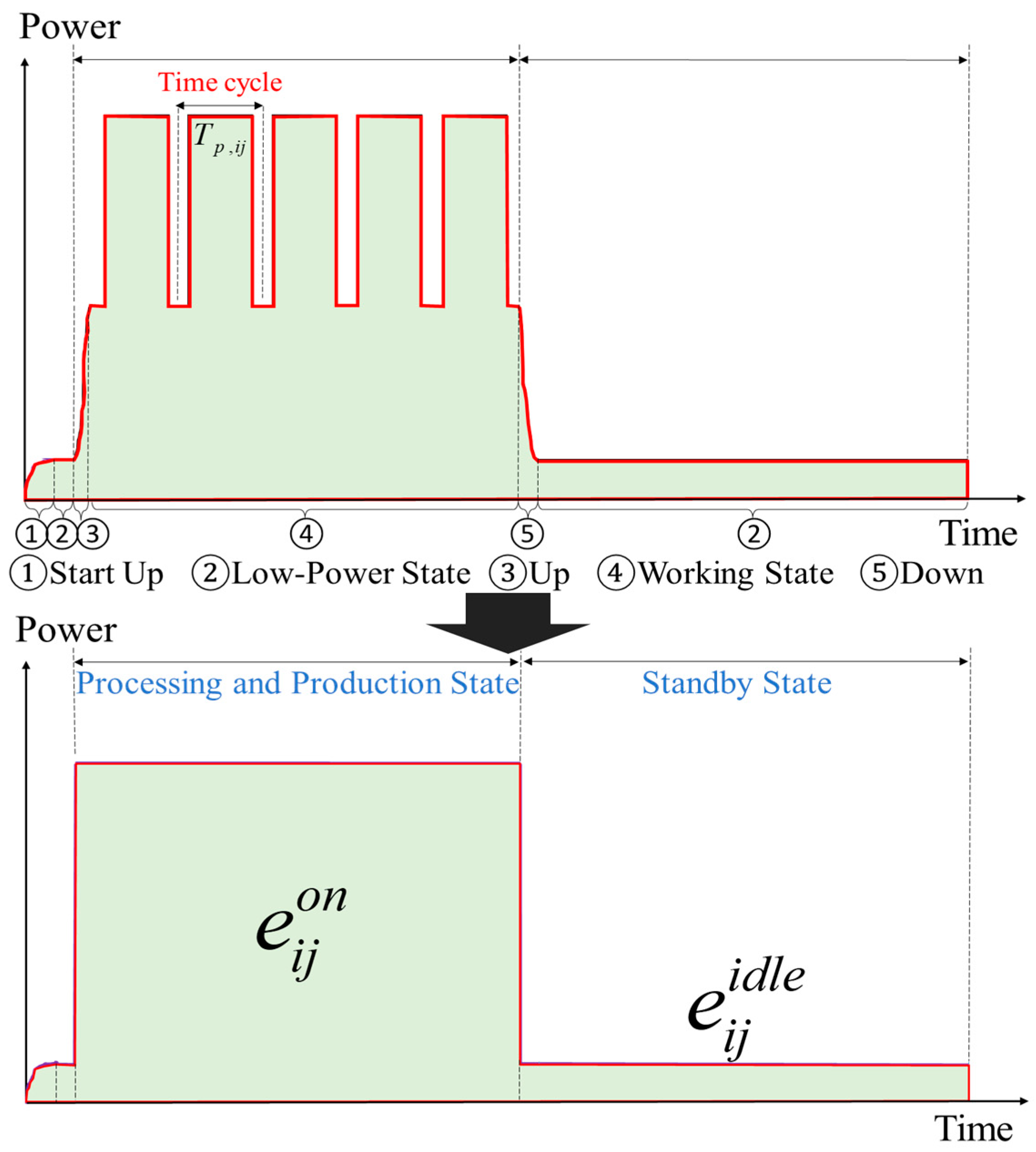
The power consumption characteristics of manufacturing machines follow distinct operational phases, as illustrated in Figure 3. Each machine transitions through five sequential states that define its energy consumption profile over time.
The machine’s operational cycle begins with a startup preparation phase, where it maintains minimal power draw in a low-power state. When production is scheduled, the machine transitions through a continuous power rise phase before reaching its steady working state. During this working state, the machine maintains constant power consumption while processing products, with each product requiring a defined processing time T p , i j .
After completing scheduled production tasks, the machine enters its shutdown sequence. Power consumption gradually decreases during this phase until the machine returns to its low-power state. We categorize these operational phases into two primary states for modeling purposes: the “processing and production state” and the “standby state”.
The total energy consumption varies significantly between these two states. During the processing and production state, energy consumption ( e i j o n ) corresponds to the shaded area of the first phase in Figure 3. The standby state consumes considerably less energy ( e i j i d l e ), as shown by the smaller shaded area in the figure’s lower portion. This equivalent power consumption representation maintains consistent energy totals while simplifying the state transition dynamics.
These power consumption patterns form the foundation for our energy-aware scheduling model, enabling precise calculation of operational costs and optimization of machine state transitions. The next section builds upon this understanding to develop comprehensive production scheduling constraints.

3.2.1. Time Discretization

The production system employs a minimum scheduling interval T s of 10 min, selected to balance control granularity with computational efficiency. Based on this interval, the total number of scheduling periods N within a 24-h operational day is calculated as:
N = 24 × 60 T s = 144

3.2.2. Processing Time and Decision Variable

As shown in Figure 3, processing time T p , i j represents the time required for the machine M i j to process a part. For each machine M i j , Z i j t is a decision variable at time t .
Z i j t = 1 , m a c h i n e   i n   p r o c e s s i n g   a n d   p r o d u c t i o n   s t a t e 0 , m a c h i n e   i n   s t a n d b y   s t a t e

3.2.3. Production Flow Management

(1) Starvation Prevention Rule: When an intermediate storage area ( B i j ) becomes empty ( B i j = 0 ), downstream machines must transition to standby state to prevent inefficient operation and energy waste. This rule ensures synchronized material flow through the production line.
(2) Overflow Prevention Rule: When an intermediate storage area ( B i j ) reaches its maximum capacity, upstream machines must enter standby state to prevent material overflow. This constraint maintains production line stability and prevents quality issues from improper material handling.
These rules form the foundation for our integrated scheduling approach, enabling simultaneous optimization of production efficiency and energy consumption. The following sections build upon this framework to detail the complete mathematical formulation for the production constraints.

3.2.4. Production Constraints

Within a given T s , each machine produces a quantity of parts   n i j t based on its processing time T p , i j :
n i j t = T s T p , i j . Z i j t
At each time slot t , the buffer level is updated as:
B i j t = B i j t 1 + n i j t i j n i j + 1 t , i = 0 , , S ; j = 1 , , M i B i j t = B i j t 1 + n i j t i j n 01 t , i = 1 , , S ; j = M i Q p t = n 04 t , Q q t = i j n i j + 1 t , i = 0 , , S ; j = 1 , , M i   Q q t = i j n 01 t , i = 1 , , S ; j = M i  
where i j represents the number of parts from buffer B i j t required for manufacturing one unit at the subsequent machine. S ,   M i are the upper limits of i and j respectively. Q p t denotes the quantity of the product p at time slot t . Q q t represents the quantity of the raw material j consumed at time slot t .
Based on the starvation prevention rule, the following pseudocode can be obtained:
i f   B i j t 1 < i j , i = 0 , , S ; j = 1 , , M i 1 ; t h e n   Z i j + 1 t = 0 ;
If   B i j t 1 is less than i j , the raw materials in the intermediate product storage area cannot meet the production conditions of the downstream machine, so this machine will enter a starved state. Its mathematical expression is as follows:
i j Z i j + 1 t B i j t 1 , i = 0 , , S ; j = 1 , , M i 1
The intermediate product storage area   B i j t 1 has a maximum capacity C i j , m a x . Based on the overflow prevention rule, the following pseudocode can be obtained:
i f   B i j t 1 = C i j , max   &   &   ( n i j t > i j ) , i = 0 , , S ; j = 1 , , M i ;   t h e n   Z i j t = 0 ;
If   B i j t is at maximum value, the downstream machine will enter a saturated state, and controlling this machine to be in a low power state is the most effective approach. Its mathematical expression is as follows:
Z i j t C i j , max B i j t 1     n i j t + i j , i = 0 , , S ; j = 1 , , M i

3.2.5. Power Balance

During each period T s , each machine can only select one working state. The energy consumption of each machine during period T s is represented as:
e i j t = e i j o n Z i j t + e i j i d l e 1 Z i j t
where e i j o n , e i j i d l e are the power demands when the machine is in different working states as shown in Figure 3. The total power demand of machines in the production line is:
E t = e i j t , t = 1 , , T
And the total machine power must meet the maximum power load limit:
E t E Max

3.2.6. Load Flexibility for DR

Non-critical machines adjust operations to exploit time-varying electricity prices. During peak price periods, machines prioritize standby states unless required for urgent orders, reducing grid dependency:
M i j M non-critical Z i j t Γ DR , t
where Γ D R , t defines the maximum number of active non-critical machines under DR.

3.3. Energy Model

3.3.1. Distributed Generation System (DGS)

The power generated by DGS supplies the machines for production, with surplus sold to the grid. DGS can be divided into non-dispatchable DGS (including solar, wind, and waste heat power plants) and dispatchable DGS (including distributed small-scale power generation units) [30]. The total electricity generated by DGS during period T s is the sum of electricity generated by dispatchable DGS E d D G S t and non-dispatchable DGS E n d D G S t :
E D G S t = E d D G S t + E n d D G S t
The power generated by non-dispatchable generation units (e.g., photovoltaic) can be predicted. Although all prediction schemes inherently have prediction uncertainties, the deviation between predicted and actual values can be compensated by purchasing (or selling) more/less power from the grid.
During period T s , the power production of dispatchable DGS is determined by decision variable Z f t . Based on the efficiency characteristics of internal combustion generators, the relationship between output power and fuel cost is expressed in quadratic form [31]:
C d D G S t = a e P f t 2 + b e P f t + c e
where C f t is the thermal power generation cost; P f t is the generator’s output power during period T s ; a e , b e , c e are the generator’s cost coefficients. Equation (15) is subsequently linearized using the piecewise linear approximation method detailed in Appendix B of [30] (the Linearization Modeling Approach) to transform the model into a MILP framework. Similarly, the piecewise GC trading rules (Equation (23)) in Section 3.4.3 have been linearized via segmented approximations to maintain model integrity.
The generator’s output and ramp constraints are:
P m i n P f t   P m a x R D P f t P f t 1 R U
where   P m i n ,   P m a x represent the lower and upper limits of output power; R D , R U respectively represent the lower and upper limits of ramp constraints.
The operational costs of DGS C DGS t are calculated as the sum of the operational costs of dispatchable generation and non-dispatchable generation units.
C DGS t = C d D G S t + C n d D G S t

3.3.2. Energy Exchange with Smart Grid

The power exchange management model governs the electricity transactions between the sustainable manufacturing facility and the smart grid. The total power demand of the facility P t o t a l t at time period T s can be expressed as:
P t o t a l t = P m a n u f t + P C C U S t P D G S t
where P m a n u f t represents the power demand from manufacturing equipment; P c c u s t denotes the power consumption of carbon capture equipment; P D G S t is the power generation from DGS.
The power exchange with the grid is subject to the following constraints:
P b u y t P s e l l t = P t o t a l t 0 P b u y t M Z p e s t 0 P s e l l t M 1 Z p e s t
where P b u y t and P s e l l t represent the power purchased from and sold to the grid respectively, M is a sufficiently large positive number, and Z p e s t is a binary variable indicating the power exchange status (1 for buying, 0 for selling).
The total cost for trading with the power grid ( C g r i d ) can be calculated as:
C g r i d = t = 1 T c b u y t P b u y t c s e l l t P s e l l t T s
where c b u y t and c s e l l t are the hourly electricity purchase and selling prices respectively.

3.4. GC Model

The GC model is designed for manufacturing facilities that act as prosumers—both consuming grid power and generating renewable energy. This dual role enables participation in GC trading through both certificate generation from renewable energy production and certificate purchasing to meet renewable energy consumption quotas.

3.4.1. GC Issuance

GC is issued based on the facility’s verified renewable energy generation. The number of certificates G g c t at time period T s is calculated as:
G g c t = P N D G S t T s / 1000
where G g c t is the number of tradable GC; P N D G S t . T s is the actual renewable energy generation; the division by 1000 converts kWh to MWh for certificate standardization.

3.4.2. Quota Obligations

The facility must meet a renewable energy quota ( G q u o t ) based on total energy consumption ( P m a n u f t + P C C U S t ) . T s :
G q u o t = κ q u o P m a n u f t + P C C U S t T s / 1000
where κ q u o is the renewable energy quota coefficient, determined by regulatory policies.

3.4.3. Trading and Revenue

The GC trading revenue R g c t is determined by comparing the facility’s certificate balance with its quota obligation:
R g c t = G g c t G q u o t c g c s t , i f   G g c t G q u o t C e r t i f i c a t e s u r p l u s G g c t G q u o t c g c b t + β p e n t G g c t G q u o t , i f   G g c t < G q u o t C e r t i f i c a t e d e f i c i t
where c g c s t is the selling price of GC; c g c b t   is the buying price of GC; β p e n t is the penalty coefficient for quota non-compliance.
This is a piecewise function, making it non-linear due to the conditional nature of the definition. To linearize the piecewise function, the binary decision variable δ g c t is defined as follows:
δ g c t = 1 when G g c G q u o , indicating a certificate surplus;
δ g c t = 0 when G g c < G q u o   , indicating a certificate deficit.
By introducing δ g c t , the expression can be rewritten in a linear form as follows:
R g c t = δ g c t G g c t G q u o t c g c s t + 1 δ g c t G g c t G q u o t c g c b t + β p e n t G g c t G q u o t
Simplifying the expression:
R g c t = G g c s t G q u o t δ g c t c g c t + 1 δ g c t c g c b t + β p e n t
The total GC trading revenue ( R g c ) is:
R g c = t = 1 T R g c t

3.5. CCUS Model

R c c u s represents the comprehensive benefits of the factory’s CCUS system implementation, including operating costs, carbon capture costs, storage costs, carbon penalty costs, and carbon benefits. Its mathematical expression is as follows [32]:
R ccus = C rev c C ope C cc C cs C pen c C ope = r ope t P t , t = 1 , , T C cc = r cc t Q cc t , t = 1 , , T C cs = r cs t Q cs t , t = 1 , , T C pen c = r tax t Q emi t Q cc i , t = 1 , , T C rev c = r pri t Q cs t , t = 1 , , T
where C o p e is the carbon capture operating cost; C c c is the carbon capture cost; C c s is the carbon storage cost;   C p e n c is the carbon penalty paid to the government;   C r e v c is carbon revenue. r o p e is the unit operating cost; r c c , r c s   are the costs per ton of CO2 for carbon capture and carbon storage respectively;   r t a x , r p r i are carbon tax and carbon price (unit: yuan/ton) respectively; Q e m i t , Q c c t , Q c s t represent the amount of CO2 emitted, captured, and stored during period T s respectively.
Q e m i t = κ e m i P f t , t = 1 , , T Q c c t = λ c a p Q e m i t , t = 1 , , T Q c s t = 1 η Q c c t , t = 1 , , T E c c u s = e c c u s Z f t , t = 1 , , T R ccus = t = 1 T R c c u s t , t = 1 , , T
where κ e m i represents the ratio of CO2 emissions to output power;   P f t is the power generation of thermal power generation units; λ c a p represents carbon capture absorption rate; η represents transportation loss rate; E c c u s is the power consumed by carbon capture; e c c u s is the power consumed by unit carbon capture equipment.

3.6. Actual Carbon Emission Calculation Model

Calculate the actual total CO2 emissions Q t o t a l t of the sustainable manufacturing facility at time   s l o t   t :
Q t o t a l t = Q e m i t + Q S G t
where Q D G S e m i t is the carbon emission from DGS equipment operation; Q S G t is the actual carbon emission from electricity purchased from the smart grid. The calculation formula is as follows:
Q S G t = E B t κ S G
where   E B t is the amount of electricity purchased from the smart grid; parameter κ S G is the grid carbon emission intensity [33].

4. Simulation Case Study Results and Discussion

4.1. Experimental Design and Scenarios Configuration

To validate the proposed low-carbon economic scheduling framework, this study investigates a large-capacity lithium-ion manufacturing plant. Building upon its industrial context, we progressively analyzed four scenarios, each integrating additional low-carbon strategies:
Scenario 1 (GC): This baseline scenario implemented traditional scheduling with GC obligations, where the objective function was configured to maximize production output, serving as a benchmark for comparison with our proposed profit maximization DR model.
Scenario 2 (GC + DR): This approach shifted the objective function from production maximization (Scenario 1) to profit maximization. By strategically rescheduling production loads to off-peak hours, it enabled peak shaving, valley filling, and the incorporation of DR.
Scenario 3 (GC + DR + DGS): The framework was expanded to include DGS, such as solar photovoltaic (PV) and thermal power units. The DGS reduces reliance on grid electricity, increases renewable energy utilization, enhances DR flexibility, and generates revenue through excess power sales.
Scenario 4 (GC + DR + DGS + CCUS): This scenario further expands the framework by comprehensively integrating CCUS technologies. The CCUS system captures CO2 emissions from the thermal power units, reducing the facility’s carbon footprint and enabling participation in carbon trading markets. This integration allows the manufacturing facility to generate additional revenue through the sale of carbon credits, while simultaneously reducing carbon tax liabilities and enhancing sustainability performance.
GC obligations were consistently incorporated across all four scenarios to align with current regulatory and market-driven trends in renewable energy adoption. This approach ensures that each scheduling strategy remains compliant with sustainability requirements while allowing for a systematic evaluation of additional low-carbon measures. By maintaining GC as a baseline, we create a fair comparative framework, enabling the isolation of benefits from DR, DGS, and CCUS without introducing discrepancies in regulatory constraints. Furthermore, the integration of GC across all cases reflects future real-world industrial conditions. Several European countries (e.g., Norway and Sweden) and U.S. states like California and New York have implemented mandatory GC quotas. Manufacturing facilities in these areas are required to comply with evolving renewable energy mandates while optimizing both production efficiency and economic performance.
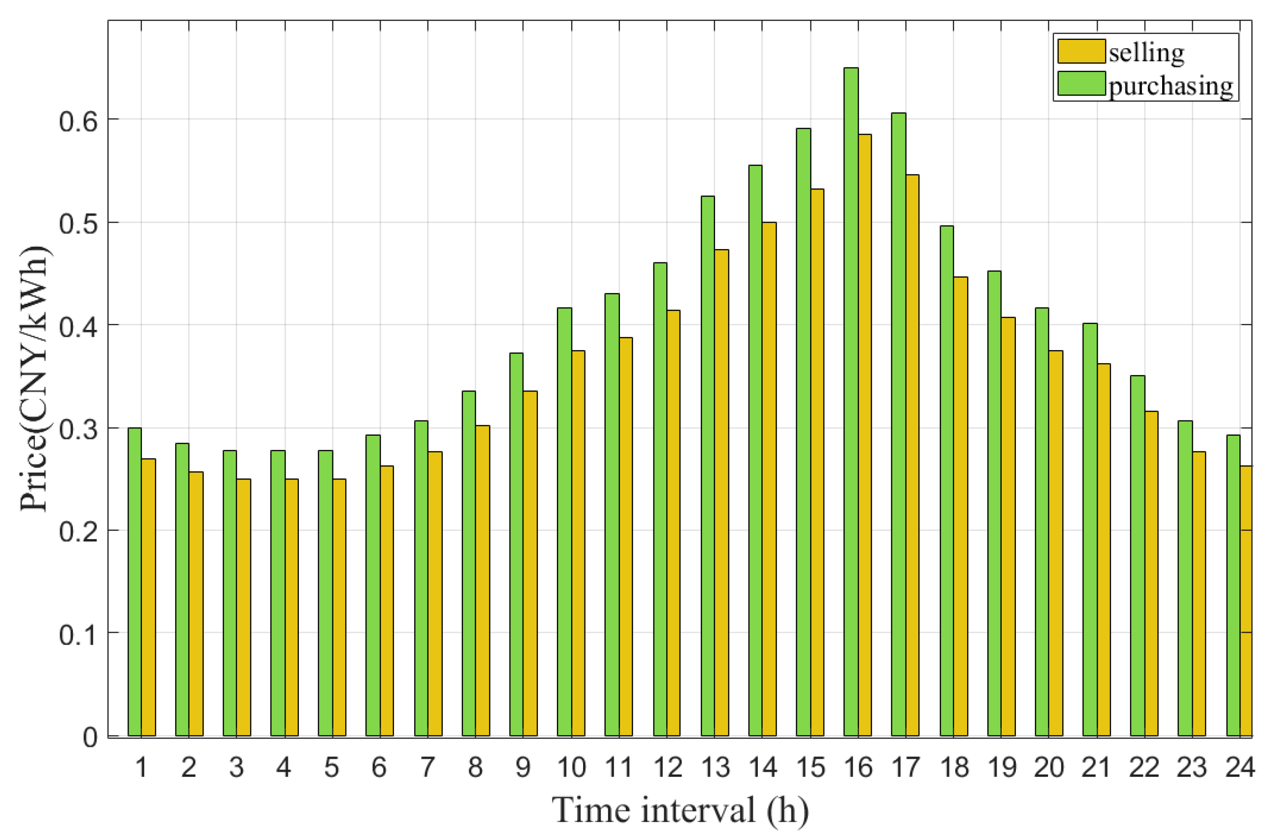
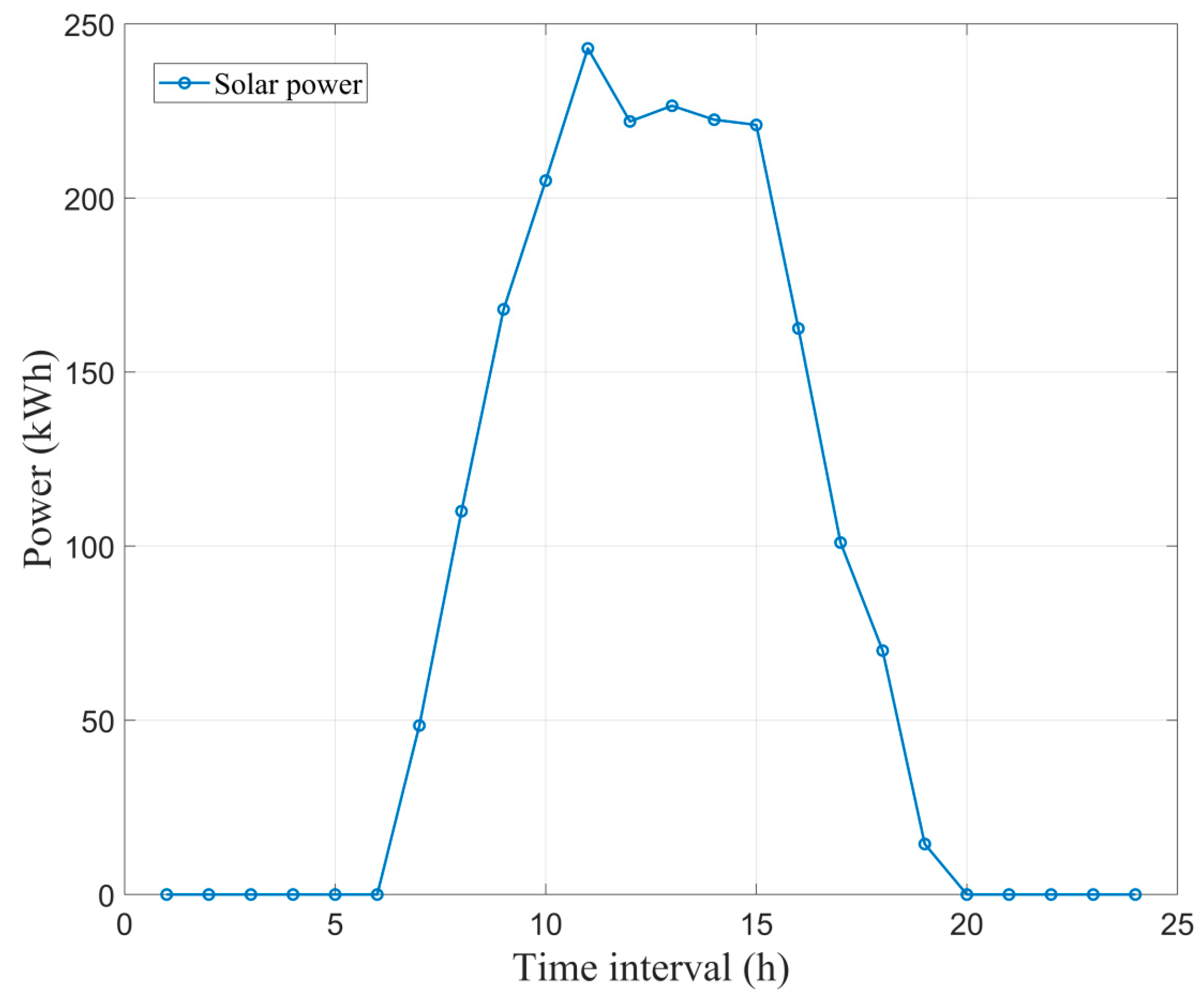
Detailed production line parameters were obtained from references [27,28,29]. To ensure the realism and practical applicability of the simulation, these referenced parameters were not used directly but were adapted and validated against industrial data. Specifically, the production times, machine power characteristics, and energy cost coefficients extracted from [27,28,29] were cross-checked with real-time operational benchmarks reported in [28]. The adjustment process involved aligning referenced parameters with typical working ranges observed in large-scale lithium-ion battery manufacturing plants, correcting discrepancies caused by experimental conditions or laboratory-scale settings. Furthermore, the validation methods presented in [28], including empirical comparison with on-site measurements and parameter consistency checks under actual manufacturing load profiles, were applied to confirm that the adapted parameters reflect realistic industrial behavior. The simulation employs a 24-h horizon, which is sufficient to capture key operational decisions in discrete manufacturing scenarios with rapid production speeds, as demonstrated in reference [28]. The electricity purchase/sale prices are illustrated in Figure 4 [30]. The renewable energy quota coefficient was 0.2 [31]. The CO2 emission coefficient for thermal power units was 1.011 [32]. The day-ahead solar power generation forecasts are shown in Figure 5 [34]. The GC trading price was set at 0.1 CNY/kWh [34]. The CCUS-related coefficients, including a carbon capture efficiency factor of 0.9 and a carbon transportation loss rate of 0.02 were obtained from references [32,35]. The thermal power unit cost coefficients were 0.0013, 0.16, and 10, respectively [36].

4.2. Comparative Analysis of Scenarios 1–4: Economic and Environmental, and Grid Stability Impacts

In this study, Lingo 12.0 is used to solve the formulated optimization problem as a MILP solver.
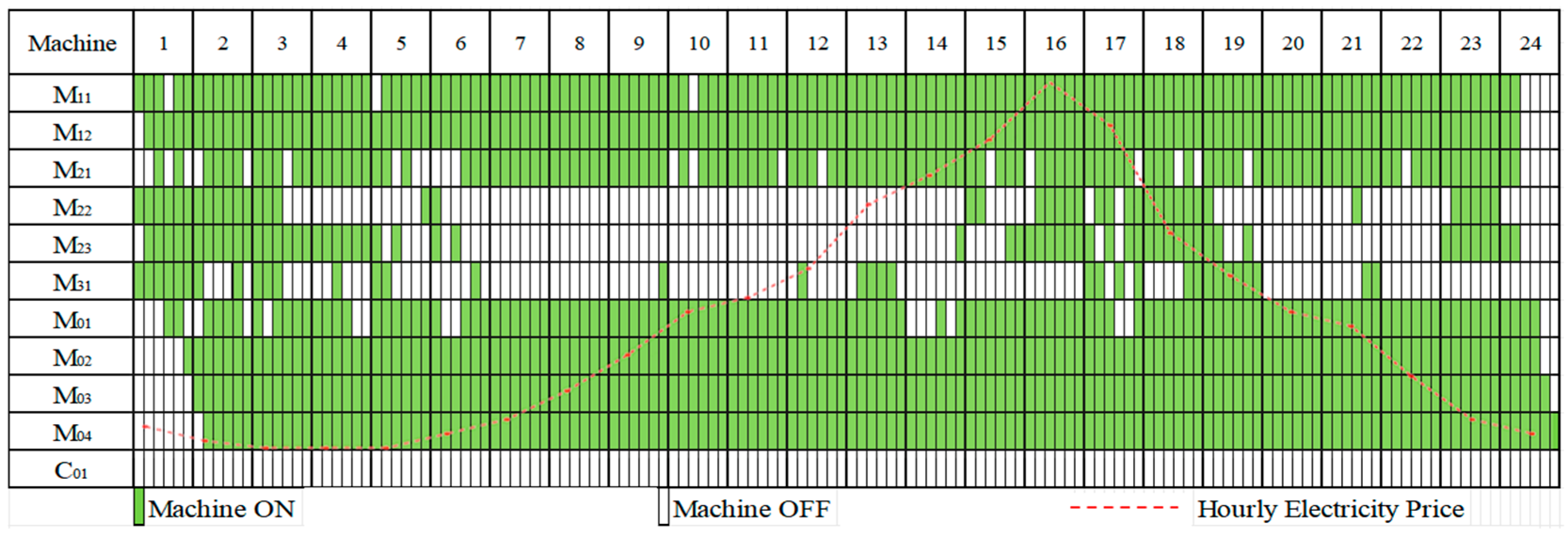
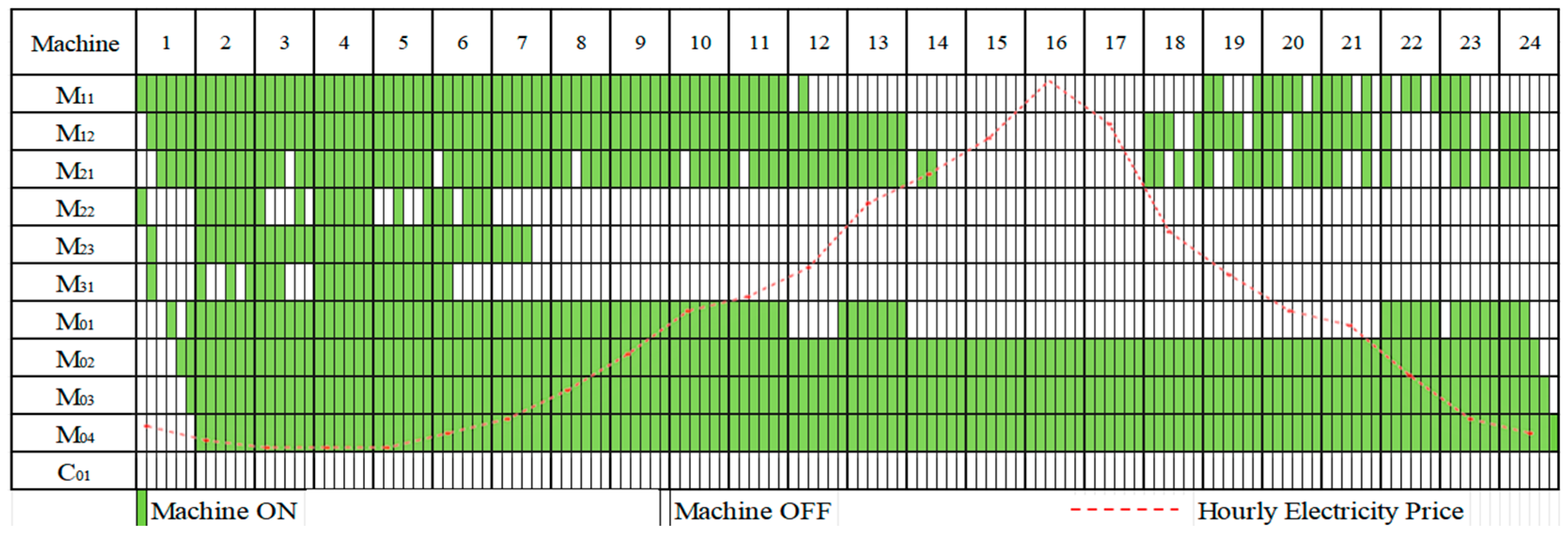
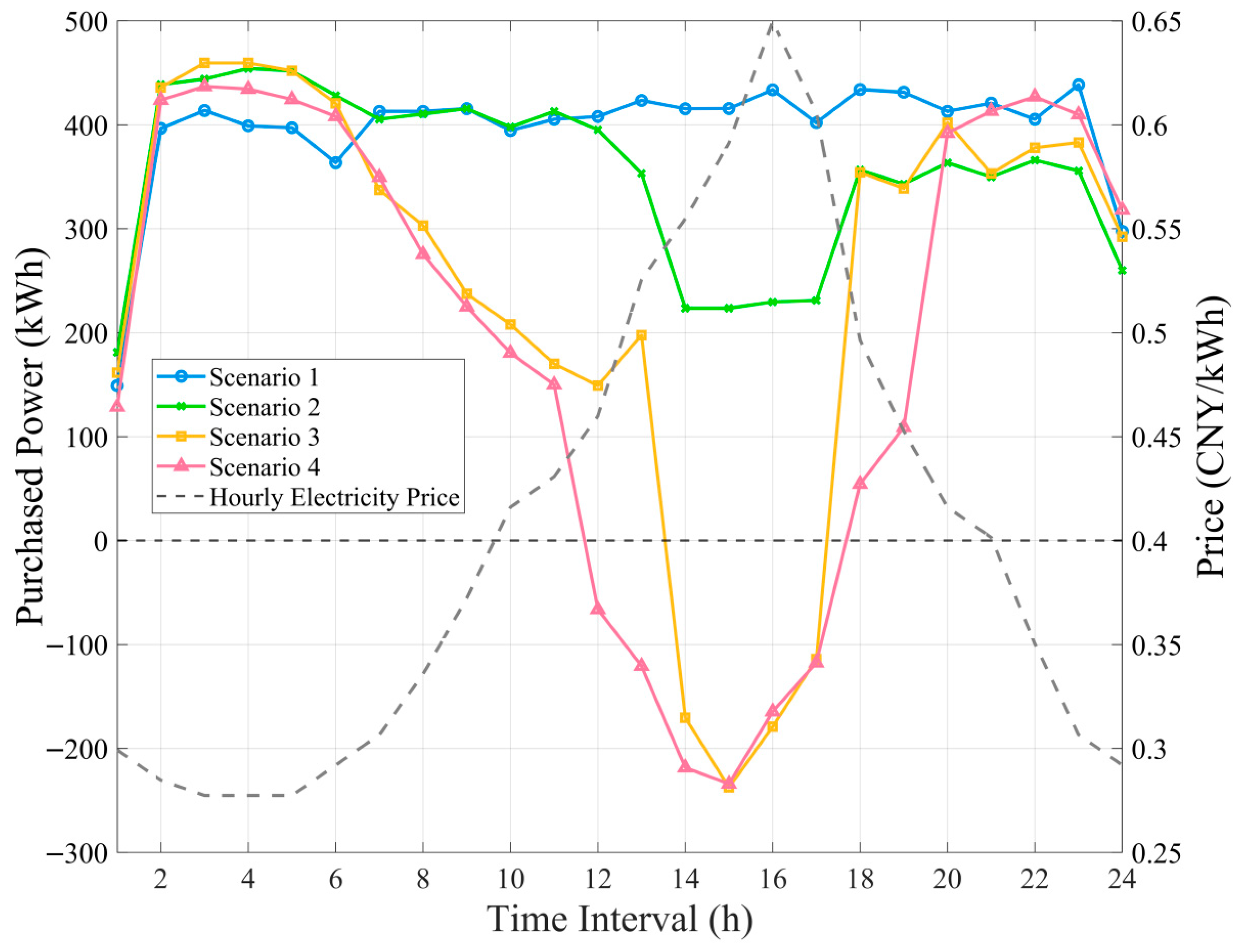
Scenario 2 vs. Scenario 1: Scenario 2 (GC+DR) achieved a profit of 20,269.9 CNY, surpassing Scenario 1 (Baseline, 17,970.9 CNY) by 12.8%, as shown in Table 1. This improvement is attributed to a key operational adjustment visible in the production line optimization plans shown in Figure 6 and Figure 7. In these figures, the numbers 1–24 in the topmost row represent the 24 h of the day, and the first column shows the manufacturing machines ( M 11 - M 04 ) and schedulable DGS (a thermal power unit, C 01 ) used in the factory. The green bars indicate processing and production state, while white spaces represent standby state for each machine and power unit across the 24-h scheduling horizon. The main difference between Figure 6 and Figure 7 is as follows: Machines (e.g., M 11 , M 12 , M 21 , M 22 , M 23 ,   M 31 , M 01 ) are strategically rescheduled to operate during low electricity price periods in Figure 7. The facility is able to reduce its energy costs while maintaining production output. This strategic adjustment is made possible through the real-time dynamic control of the production line’s power consumption, enabling DR, which helps reduce peak-hour consumption. As shown in Figure 8, Scenario 2 results in a 45.6% reduction in peak-hour (14:00–17:00) power consumption compared to Scenario 1. This reduction not only leads to significant cost savings but also contributes to a more stable and efficient power grid by decreasing demand during high-stress periods, highlighting the effectiveness of DR in optimizing both production and energy use.
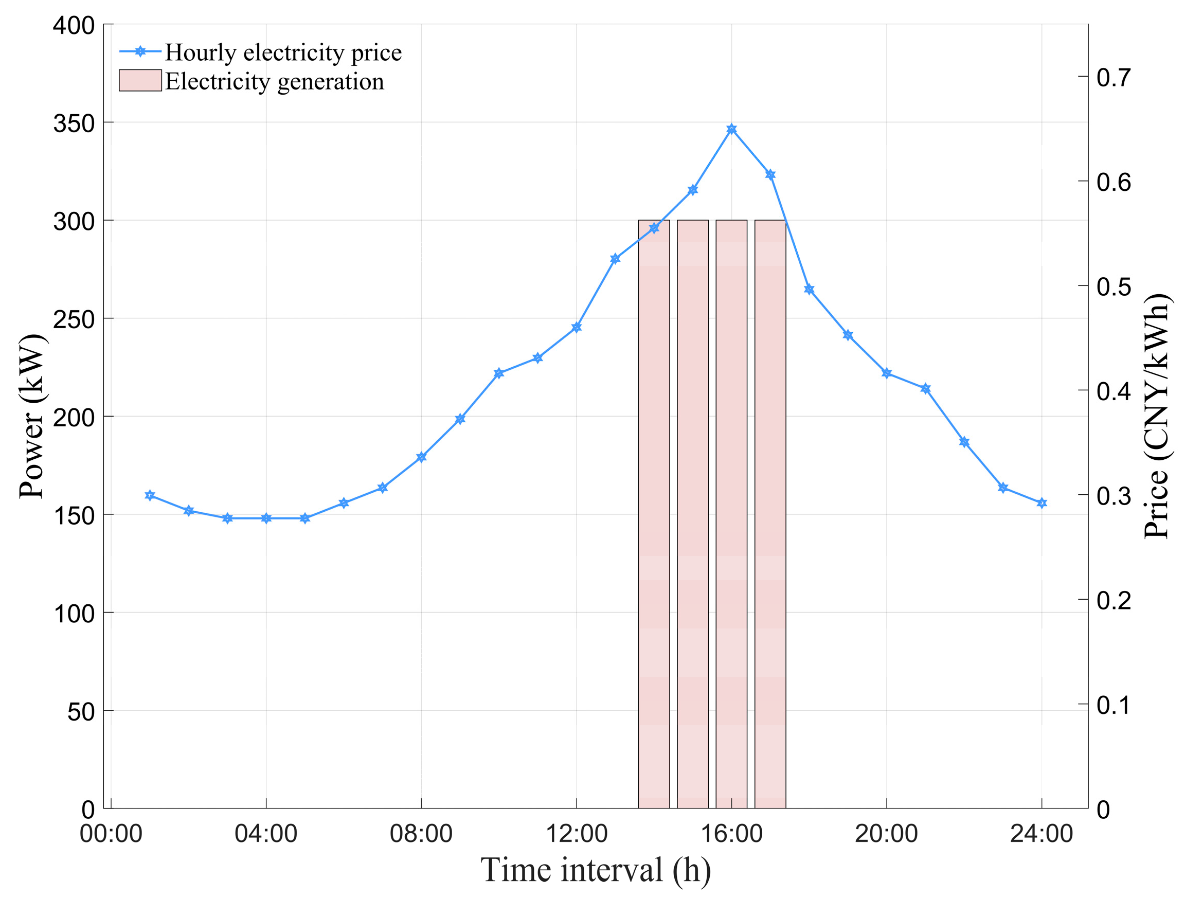
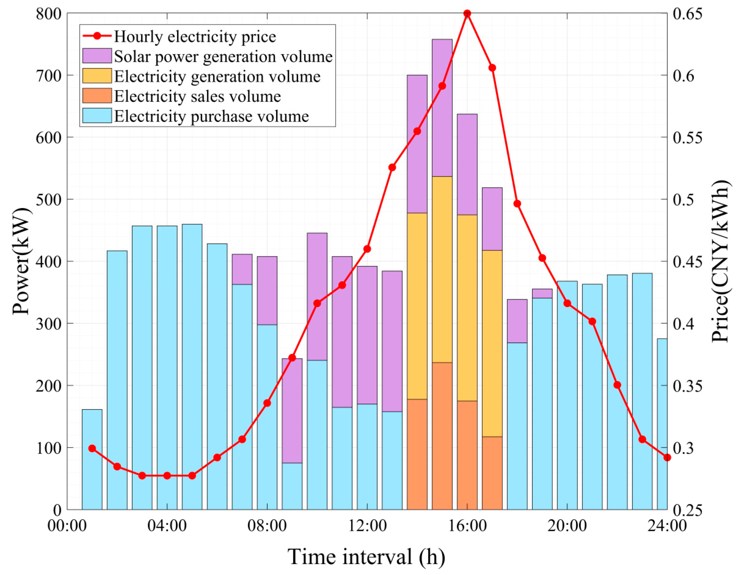
Scenario 3 vs. Scenario 2: Scenario 3 (GC + DR + DGS) achieved a profit increase to 22,615.4 CNY, which is 11.6% higher than Scenario 2 (20,269.9 CNY), primarily through the integration of DGS, including both solar and thermal power units. As shown in Table 1, the total electricity generation from DGS in Scenario 3 was 3214.5 kWh, while there was no DGS generation in Scenario 2. The DGS reduced the facility’s reliance on grid power, as evidenced by the lower grid electricity purchases in Scenario 3 compared to Scenario 2 in Figure 8. The reduced grid consumption also led to a 24.0% decrease in total carbon emissions from 5.9917 t in Scenario 2 to 4.5562 t in Scenario 3 (Table 1). Figure 9 shows that during peak price periods (14:00–17:00), the thermal power units in the DGS operated at maximum capacity due to their lower generation costs compared to grid electricity prices. Additionally, as illustrated in Figure 10, the solar photovoltaic systems (PV) in the DGS generated renewable electricity during daylight hours, further reducing grid power consumption and contributing to overall cost reduction. Importantly, the total production quantity remained constant at 828 pieces in both Scenarios 2 and 3 (Table 1), indicating that the economic and environmental benefits from DGS integration were achieved without compromising production output. The system’s ability to sell its excess distributed generation back to the grid during peak price periods (14:00–17:00) as shown in Figure 10, further generated additional revenue. This demonstrates how integrated DGS, including both solar and thermal power, can create value through cost reduction, revenue generation, enhanced sustainability, and reduced carbon emissions while maintaining production levels.
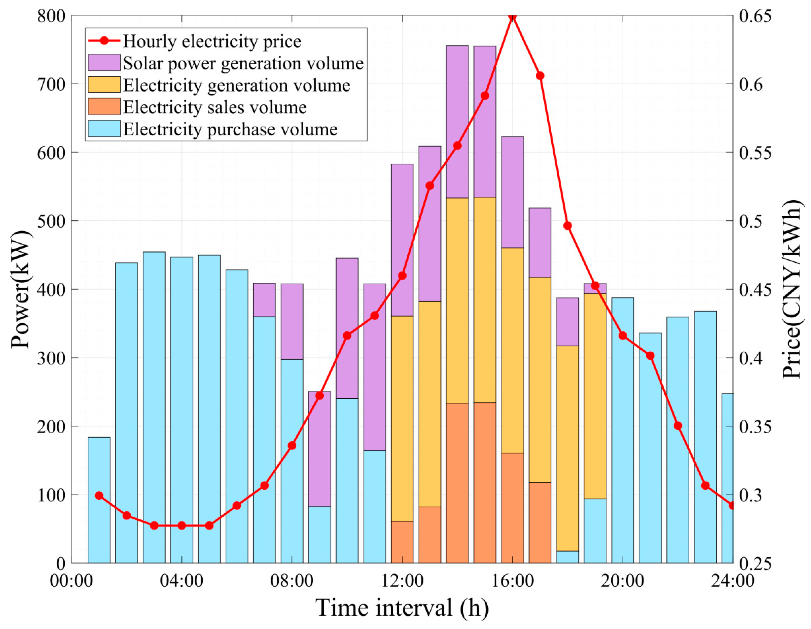
Scenario 4 vs. Scenario 3: Scenario 4 (GC+ DR+DGS+CCUS) represents the most comprehensive integration, achieving the highest profit of 25,517.9 CNY (12.8% above Scenario 3’s 22,615.4 CNY) as shown in Table 1. The integration of CCUS extends the clean operational window of thermal power units, shifting from the traditional peak demand period (14:00–17:00) to a broader timeframe (12:00–19:00), as illustrated in Figure 10 and Figure 11. Far from promoting prolonged fossil fuel dependency, this shift leverages CCUS to decarbonize thermal power generation, capturing 2.1816 tons of CO2 daily and reducing net emissions by 23.1% compared to the non-CCUS scenario (from 4.5562 t to 3.5025 t). By enabling operation during off-peak hours, CCUS enhances system flexibility, displaces high-carbon grid electricity, and supports a 45.6% reduction in peak-hour consumption. Economically, this extension boosts profitability by 12.8% (from 22,615.4 CNY to 25,517.9 CNY) through carbon market revenues and CO2 utilization (e.g., CO2-EOR), which will be detailed in Section 4.3. This demonstrates that CCUS does not merely extend thermal power use but transforms it into a sustainable energy option, facilitating industrial decarbonization while maintaining grid stability and economic competitiveness. Production output declined marginally by 2.17% (810 units in Scenario 4 vs. 828 units in Scenarios 1–3). This reduction stems from the proposed model’s prioritization of profit over production volume: when selling excess electricity to the grid yields higher financial returns than utilizing it for additional battery manufacturing, the system autonomously reduces battery production to optimize overall revenue. From the perspective of production plans and contractual obligations, such reductions are generally acceptable in flexible manufacturing setups, such as battery production, as they leverage buffer inventories to enable short-term optimizations without breaching contracts. However, to mitigate risks of non-compliance or supply disruptions, the model can incorporate safeguards such as predefined minimum production thresholds based on contractual demands, ensuring alignment with operational commitments. Despite the marginal decrease in production, the total DGS electricity generation increased by 37.3% from 3214.5 kWh in Scenario 3 to 4414.5 kWh in Scenario 4. Scenario 4 achieved the highest profits and lowest emissions among all scenarios evaluated, highlighting the synergistic benefits of integrating DR, DGS, and CCUS technologies in sustainable manufacturing.
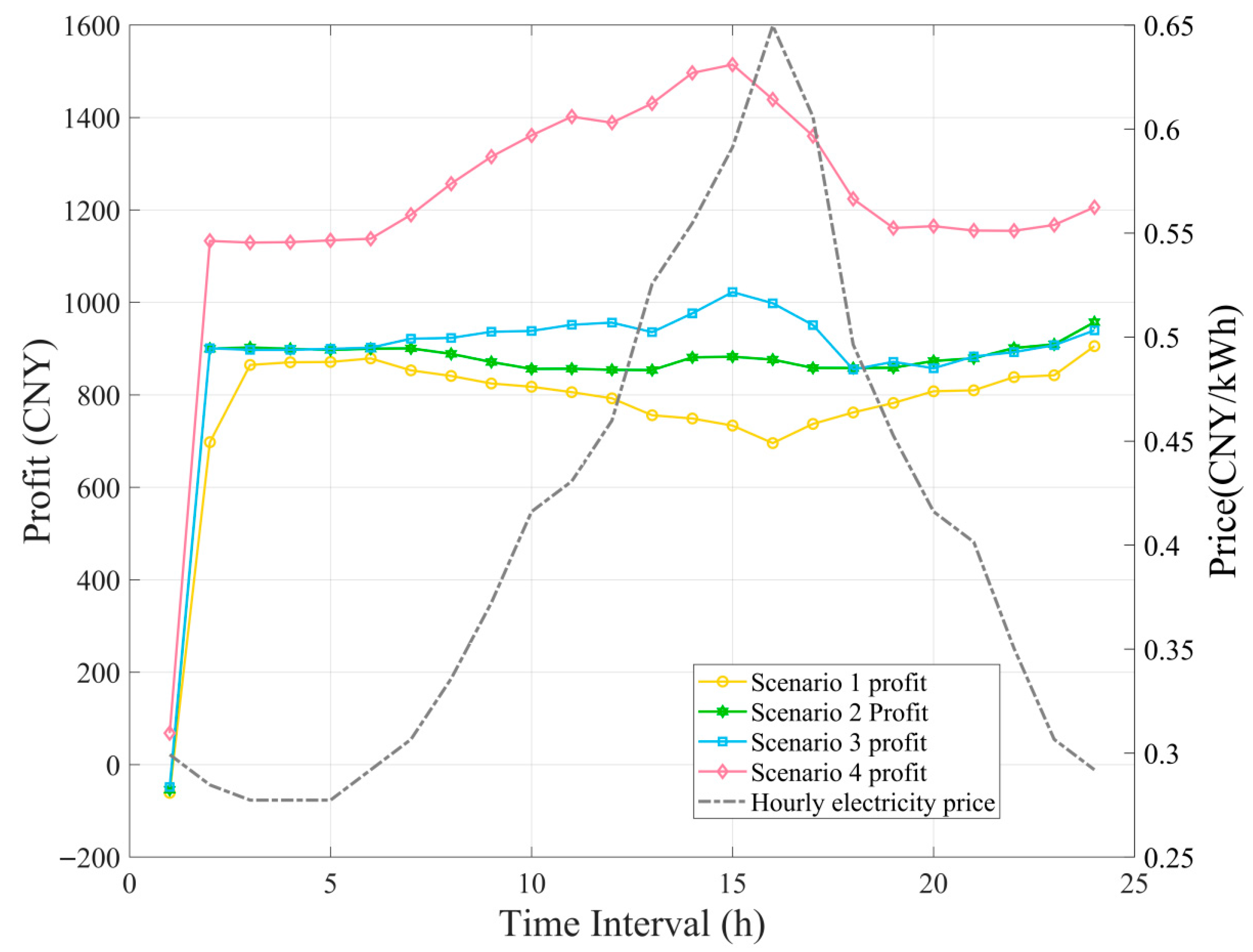
Figure 12 illustrates the hourly profit distribution across all four scenarios over a 24-h period. During peak electricity price hours (09:00–17:00), Scenarios 3 and 4 demonstrate notably higher profits compared to Scenarios 1 and 2, primarily due to their integration of DGS and CCUS technologies. Scenario 1 exhibits the lowest profit profile, especially during high-price periods (14:00–17:00), due to inefficient energy management and the requirement to purchase GC to meet renewable energy quotas. Scenario 2 shows improved profit performance by strategically implementing DR measures, though it remains constrained by GC purchasing obligations. Scenario 3 achieves increased profits through the synergistic benefits of DR and DGS, which reduce reliance on grid electricity and generate additional revenue through excess power sales. Scenario 4 demonstrates the highest profit margins, particularly during peak hours, by leveraging the comprehensive integration of CCUS technology alongside DR and DGS. This enables participation in multiple environmental markets, including carbon trading, creating new revenue streams while simultaneously reducing emissions and enhancing overall sustainability performance.

4.3. Computational Performance

Scenario 4 represents the complete proposed framework and is therefore the most complex instance of the MILP model. For this scenario, the model comprises 2726 decision variables and 3507 constraints, primarily encompassing binary variables for equipment states (e.g., machine on/standby, grid buy/sell, GC surplus/deficit), continuous variables for energy flows (e.g., power generation, consumption, and trades), all with high temporal coupling across the 24-h horizon. The model was solved using Lingo 12.0 on a PC equipped with an Intel(R) Core(TM) i5-12400F CPU, 32.0 GB RAM, running Windows 10 Pro. Over 100 independent runs of Scenario 4, the solver achieved an average convergence time of 16.465 s, with an optimality gap consistently below 2%. This performance confirms the computational tractability of even the full framework, supporting its potential for real-time or near-real-time industrial deployment. If stronger real-time capabilities are required, adopting a newer version of the solver and better computer hardware would further reduce convergence times and enhance efficiency.

5. Conclusions and Future Work

This study proposes a novel profit-driven framework for low-carbon scheduling in sustainable manufacturing, integrating GC, DR, DGS, and CCUS. Through a lithium-ion battery manufacturing case study in Northwest China, the framework demonstrated significant economic and environmental synergies: a 42.0% profit increase and a 45.1% reduction in CO2 emissions, with a minimal production loss of 2.17%. This outcome underscores the model’s inherent capability to balance economic objectives against production volume, where the marginal profit gain significantly outweighs the minimal output reduction. Key innovations include a unified mathematical model that harmonizes manufacturing processes, energy systems, and carbon management across electricity, carbon, and GC markets.
We acknowledge, however, that the current model does not fully capture certain subsystem interdependencies—for instance, no direct variables link CCUS operation with DR. To address these limitations and deepen the integration of system components, future work will focus on:
  • Incorporating stochastic modeling of market and technical uncertainties for improved framework assessment and extending the simulation horizon to multi-day or weekly periods with dynamic carbon market operations to enhance credibility in depicting longer industrial cycles and market fluctuations;
  • Developing explicit coupling mechanisms, such as direct variables linking CCUS operations with DR, to enhance subsystem interdependencies;
  • Implementing minimum production quotas as a hard constraint to ensure operational commitments are fully met.
Additionally, while the proposed model is currently validated in discrete manufacturing systems, future efforts will extend its application to continuous process sectors (e.g., chemicals, steel) and explore the integration of energy storage for improved load balancing and flexibility. Scaling this framework to industrial parks could further amplify its benefits through shared CCUS infrastructure and cross-facility energy coordination. To further validate the framework’s practical feasibility under operational conditions, we plan to conduct a real industrial case study incorporating empirical data from operational industrial settings.

Author Contributions

Y.-C.L., M.W., R.H. and L.C. (Lu Chen): Writing—review and editing, Writing—original draft, Visualization, Software, Methodology, Formal analysis, Data curation. X.W. and X.X.: Writing—review and editing, Validation, Supervision, Project administration, Methodology, Investigation, Funding acquisition, Conceptualization. M.J., L.C. (Lijie Cui), Z.J. (Zhiyang Jia) and Z.J. (Zhong Jin): Writing—review and editing, Funding acquisition. All authors have read and agreed to the published version of the manuscript.

Funding

This work was supported by the National Natural Science Foundation of China under Grants 61802184 and 62562065, Natural Science Foundation of Xinjiang Uygur Autonomous Region (2023D01F42), “Tianshan Elite” Training Program of Xinjiang Uygur Autonomous Region (No. TSYC202301B163), Research Foundation of China University of Petroleum-Beijing at Karamay (No. XQZX20220004, XQZX20240011), Tian-Chi Talents Project of Xinjiang Uygur Autonomous Region, Innovative Outstanding Young Talents Project of Karamay, Jiang Min High-Level Talent Studio Project of Karamay.

Data Availability Statement

The data underlying this article are available in this article and its references.

Acknowledgments

The authors would like to express their sincere gratitude to the interviewed experts for their time and invaluable knowledge sharing as well as the referees who provided helpful insights.

Conflicts of Interest

Author Lu Chen was employed by the PetroChina Xinjiang Oilfield Company. The remaining authors declare that the research was conducted in the absence of any commercial or financial relationships that could be construed as a potential conflict of interest. The authors declare that they have no known competing financial interests or personal relationships that could have appeared to influence the work reported in this paper.

Nomenclature

t, T, NTime period index, total periods, scheduling periods per day
i, j, p, qBranch index, position index, product index, raw material index
S ,   M i , P, QMax branch index, max position index in branch i, total types of products, total types of raw materials
T s ,   T p , i j Scheduling interval, processing time for machine M i j
Π total Total profit
λ p t ,   Q p t Market price and quantity of the product p
c q t ,   Q q t Unit cost and the quantity of the raw material q consumed
M i j ,   Z i j t Machine at (i,j), binary state (1 = on, 0 = standby)
n i j t Parts produced by M i j at time t
e i j o n , e i j i d l e ,   e i j t Power in processing, standby, and total at time t
B i j , B i j t Buffer at (i,j), buffer level at time t
C i j , max ,   i j Max buffer capacity, parts needed per downstream unit
M non-critical ,   Γ DR , t Non-critical machines, max active machines in DR
E t ,   E Max Total power demand, maximum load limit
E D G S t ,   E n d D G S t ,   E d D G S t DGS total, non-dispatchable, dispatchable generation
P f t ,   C f t Generator output power, thermal generation cost
a e ,   b e ,   c e Generator cost coefficients (quadratic, linear, constant)
P m i n , P m a x , RD, RUPower limits (min, max), ramp limits (down, up)
Z f t Binary variable for dispatchable DGS
P t o t a l t , P m a n u f t ,   P C C U S t ,   P D G S t Power of facility total, manufacturing, CCUS, DGS
  P b u y t ,   P s e l l t , Z p e s t Grid purchase, sale, binary status (1 = buy, 0 = sell)
C g r i d ,   C DGS t , C Grid t Grid trading cost, DGS cost, grid transaction cost
c b u y t ,   c s e l l t Electricity purchase and selling prices
MLarge positive number for big-M constraints
G g c t ,   G q u o t Tradable certificates, renewable energy quota
P N D G S t ,   κ q u o Renewable generation, quota coefficient
c g c s t ,   c g c b t ,   β p e n t GC selling price, buying price, penalty coefficient
δ g c t Binary GC status (1 = surplus, 0 = deficit)
R g c ,   R gc t Total GC revenue, GC revenue at time t
R ccus ,   R ccus t Total CCUS benefits, CCUS revenue at time t
C rev c ,   C ope , C cc ,   C cs ,   C pen c Carbon revenue, operating, capture, storage, penalty costs
r ope ,   r cc ,   r cs Unit operating, capture, storage costs
r tax ,   r pri Carbon tax, carbon price
Q emi t , Q cc t , Q cs t CO2 emitted from DGS, captured, stored at time t
Q t o t a l t ,   Q S G t Total emissions, grid electricity emissions at time t
κ e m i , λ c a p , ηEmission ratio, capture rate, transport loss rate
E c c u s ,   e c c u s Total capture power, unit capture equipment power
E B t ,   κ S G Grid electricity purchased, grid emission intensity

References

  1. Fan, J.L.; Li, Z.Z.; Huang, X.; Li, K.; Zhang, X.; Lu, X.; Wu, J.Z.; Hubacek, K.; Shen, B. A net-zero emissions strategy for China's power sector using carbon-capture utilization and storage. Nat. Commun. 2023, 14, 5972. [Google Scholar]
  2. Carmona-Martínez, A.A.; Rueda, A.; Jarauta-Córdoba, C.A. Deep decarbonization of the energy intensive manufacturing industry through the bioconversion of its carbon emissions to fuels. Fuel 2024, 371, 1922. [Google Scholar] [CrossRef]
  3. Su, X.N.; Liu, P.F.; Mei, Y.D.; Qiu, J.X. The impact of carbon capture, utilization, and storage (CCUS) projects on environmental protection, economic development, and social equity. J. Clean. Prod. 2024, 482, 144218. [Google Scholar] [CrossRef]
  4. Luo, L.; Li, Y.; Wei, L. Use of metaverse technology clusters and quantum computing in CCUS: Research status and trends. Xinjiang Oil Gas 2023, 19, 86–94. [Google Scholar]
  5. Hensel, J.; Mangiante, G.; Moretti, L. Carbon pricing and inflation expectations: Evidence from France. J. Monet. Econ. 2024, 147, 103593. [Google Scholar]
  6. Li, J.K.; Ge, S.Y.; Liu, H.; Yu, Q.; Zhang, S.D.; Wang, C.S.; Gu, C.H. An electricity and carbon trading mechanism integrated with TSO-DSO-prosumer coordination. Appl. Energy 2024, 356, 122328. [Google Scholar]
  7. Nie, Y.; Zhang, G.; Zhong, L.; Su, B.; Xi, X. Urban-rural disparities in household energy and electricity consumption under the influence of electricity price reform policies. Energy Policy 2024, 184, 113868. [Google Scholar] [CrossRef]
  8. Shu, Y.; Dai, Y. The synergetic competition of cross-regional integrated energy systems with low-carbon technology heterogeneity under carbon emission trading mechanism to achieve carbon reduction target. Renew. Energy 2024, 236, 121394. [Google Scholar]
  9. Wang, L.; Xian, R.; Jiao, P.; Chen, J.; Chen, Y.; Liu, H. Multi-timescale optimization of integrated energy system with diversified utilization of hydrogen energy under the coupling of green certificate and carbon trading. Renew. Energy 2024, 228, 120597. [Google Scholar] [CrossRef]
  10. Liang, T.; Chai, L.; Tan, J.; Jing, Y.; Lv, L. Dynamic optimization of an integrated energy system with carbon capture and power-to-gas interconnection: A deep reinforcement learning-based scheduling strategy. Appl. Energy 2024, 367, 123390. [Google Scholar] [CrossRef]
  11. Wang, L.; Ma, Y.; Wang, S.; Dong, W.; Ni, L.; Liu, Z. Master-slave game-based optimal scheduling strategy for integrated energy systems with carbon capture considerations. Energy Rep. 2025, 13, 780–788. [Google Scholar]
  12. Zhang, Y.; Zhang, P.; Du, S.; Dong, H. Economic Optimal Scheduling of Integrated Energy System Considering Wind–Solar Uncertainty and Power to Gas and Carbon Capture and Storage. Energies 2024, 17, 2770. [Google Scholar] [CrossRef]
  13. Hu, J.; Wang, Y.; Dong, L. Low carbon-oriented planning of shared energy storage station for multiple integrated energy systems considering energy-carbon flow and carbon emission reduction. Energy 2024, 290, 130139. [Google Scholar] [CrossRef]
  14. Wu, W.; Du, Y.; Qian, H.; Fan, H.; Jiang, Z.; Huang, S.; Zhang, X. Industrial Park low-carbon energy system planning framework: Heat pump based energy conjugation between industry and buildings. Appl. Energy 2024, 369, 123594. [Google Scholar] [CrossRef]
  15. Xu, D.; Hu, A.Y.; Lam, C.S.; Yang, X.D.; Jin, X.L. Cooperative Planning of Multi-Energy System and Carbon Capture, Utilization and Storage. IEEE Trans. Sustain. Energy 2024, 15, 2718–2732. [Google Scholar] [CrossRef]
  16. Yuan, Z.; Zhang, H.; Cheng, H.; Zhang, S.; Zhang, X.; Lu, J. Low-carbon oriented power system expansion planning considering the long-term uncertainties of transition tasks. Energy 2024, 307, 132759. [Google Scholar]
  17. Zhao, N.; Gu, W. Low-carbon planning and optimization of the integrated energy system considering lifetime carbon emissions. J. Build. Eng. 2024, 82, 108178. [Google Scholar]
  18. He, B.; Liu, R.X.; Li, T.Y. Integrated carbon footprint with cutting parameters for production scheduling. J. Clean. Prod. 2023, 412, 137307. [Google Scholar] [CrossRef]
  19. Jin, S.S.; Wang, B.Y.; Zhang, G.; Fan, X.Y.; Jiang, S.Q.; Cao, M.Y.; Wang, Y.L. Research on Low-Carbon-Emission Scheduling of Workshop under Uncertainty. Appl. Sci. 2024, 14, 4976. [Google Scholar]
  20. Liu, H.X.; Zhuang, P.T.; Zhang, J.S.; Hu, K.X. Optimizing Low-Carbon Job Shop Scheduling in Green Manufacturing with the Improved NSGAII Algorithm. In Industrial Engineering and Industrial Management, Proceedings of the 5th International Conference, IEIM 2024, Nice, France, 10–12 January 2024; Springer: Cham, Switzerland; Volume 2070, pp. 76–86.
  21. Zhang, C.X.; Liu, C.H.; Mao, H.Y.; Tian, G.D.; Jiang, Z.G.; Cai, W.; Wang, W.B. Integration of lean production and low-carbon optimization in remanufacturing assembly. Adv. Eng. Inform. 2024, 62, 102789. [Google Scholar]
  22. Birge, J.R.; Louveaux, F. Introduction to Stochastic Programming; Springer: New York, NY, USA, 2011. [Google Scholar]
  23. Campi, M.C.; Garatti, S. Introduction to the Scenario Approach; Society for Industrial and Applied Mathematics: Philadelphia, PA, USA, 2018. [Google Scholar]
  24. Rockafellar, R.T.; Uryasev, S. Conditional value-at-risk for general loss distributions. J. Bank. Financ. 2002, 26, 1443–1471. [Google Scholar]
  25. Ju, L.; Yin, Z.; Lu, X.; Yang, S.; Li, P.; Zhang, Z.; Amjady, N. Risk-averse stochastic capacity planning and P2P trading collaborative optimization for multi-energy microgrids considering carbon emission limitations: An asymmetric Nash bargaining approach. Appl. Energy 2024, 357, 122505. [Google Scholar]
  26. Li, Z.; Xu, Y.; Wang, P.; Xiao, G. Weather routing based multi-energy ship microgrid operation under diverse uncertainties: A risk-averse stochastic approach. IEEE Trans. Smart Grid 2025, 16, 4648–4659. [Google Scholar] [CrossRef]
  27. IEC TS 62872-1:2019; Industrial-Process Measurement, Control and Automation—Part 1: System Interface Between Industrial Facilities and the Smart Grid. International Electrotechnical Commission: Geneva, Switzerland, 2019.
  28. Li, Y.C.; Hong, S.H. Real-Time Demand Bidding for Energy Management in Discrete Manufacturing Facilities. IEEE Trans. Ind. Electron. 2017, 64, 739–749. [Google Scholar]
  29. Siemens. E-Book of Siemens Battery Manufacturing Process. 2024. Available online: https://resources.sw.siemens.com/en-US/e-book-battery-operational-efficiency-across-battery-manufacturing-process (accessed on 15 January 2025).
  30. Ding, Y.M.; Hong, S.H.; Li, X.H. A Demand Response Energy Management Scheme for Industrial Facilities in Smart Grid. IEEE Trans. Ind. Inform. 2014, 10, 2257–2269. [Google Scholar] [CrossRef]
  31. Li, J.; Liu, Y.; He, J.; Shao, X. Synergistic carbon reduction effect and simulation of electricity market considering the green certificate and carbon emission trading. J. Univ. Shanghai Sci. Technol. 2024, 46, 464–474. [Google Scholar]
  32. Xuan, A.; Shen, X.W.; Guo, Q.L.; Sun, H.B. Two-Stage Planning for Electricity-Gas Coupled Integrated Energy System With Carbon Capture, Utilization, and Storage Considering Carbon Tax and Price Uncertainties. IEEE Trans. Power Syst. 2023, 38, 2553–2565. [Google Scholar]
  33. Brown, S.; Jones, D.; Fulghum, N.; Bruce-Lockhart, C.; Candlin, A.; Ewen, M.; Czyżak, P.; Rangelova, K.; Heberer, L.; Rosslowe, C.; et al. European Electricity Review 2024. Available online: https://ember-climate.org/insights/research/european-electricity-review-2024/ (accessed on 15 January 2025).
  34. Chen, X.L.; Cao, X.; Chen, J.; Liu, J.; Zhao, Y.; Bao, H. Green Certificate—Thermal power flexible response under the carbon trading mechanism of the park integrated energy system optimization. China Electr. Power 2024. Available online: https://doaj.org/article/9ee8f17f71a24d2d811dcebe6ee6199b (accessed on 15 January 2025).
  35. Yao, F.; Zhao, D.; Jia, C.; Zhao, S.; Chen, H.; Zheng, Q. Cost and Benefit Analysis of CCUS Application for Thermal Power Units in The Context of Clean Energy Market. In Proceedings of the 8th Asia Conference on Power and Electrical Engineering (ACPEE), Tianjin, China, 14–16 April 2023; pp. 1355–1360. [Google Scholar]
  36. Wang, H.; Li, K.; Zhang, C.; Ma, X. Distributed cooperative optimal operation strategy of community integrated energy system based on Stackelberg game. Proc. CSEE 2020, 40, 5435–5445. [Google Scholar]
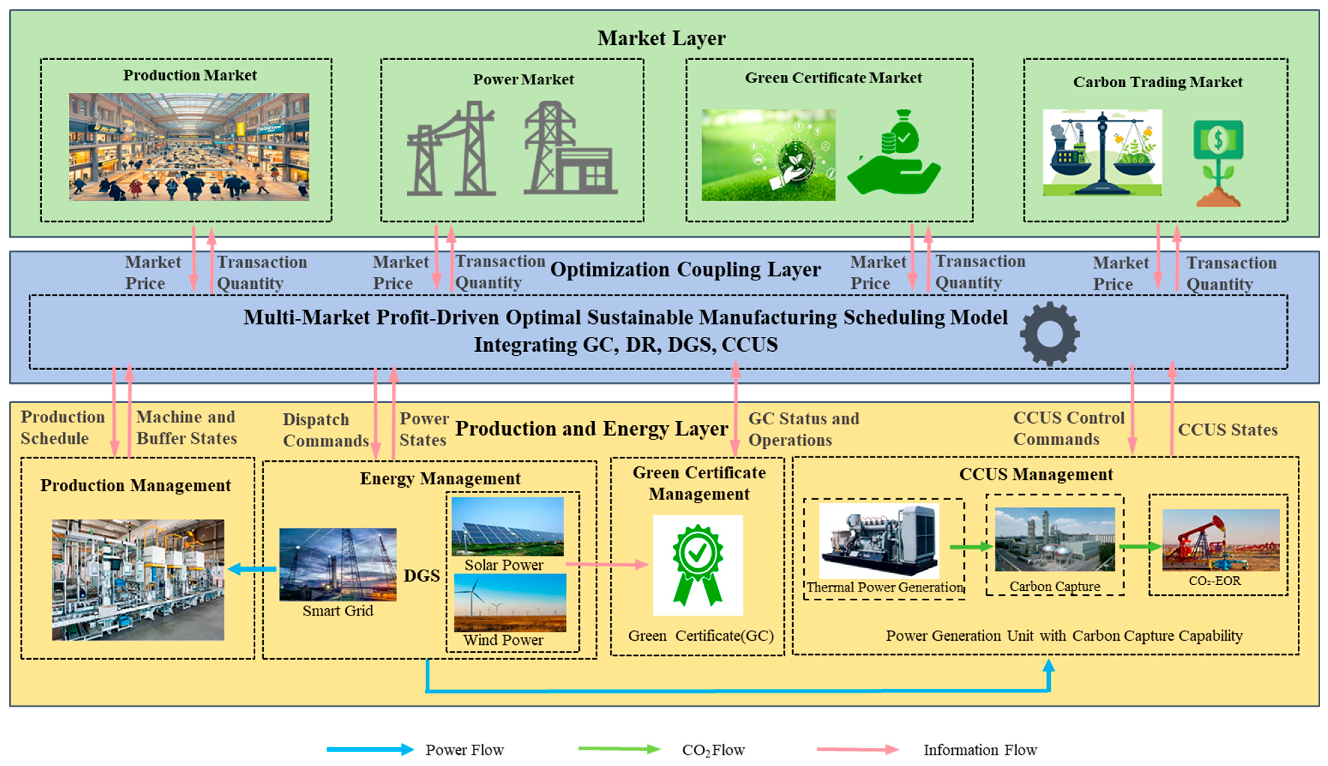
Figure 1. System framework for sustainable manufacturing.
Energies 18 06517 g001
Figure 2. Structure diagram of a lithium-ion battery production line.
Energies 18 06517 g002
Figure 3. Power consumption profile analysis of manufacturing equipment: phase-based operational states and energy distribution patterns.
Energies 18 06517 g003
Figure 4. The electricity purchase/sale prices from the grid.
Energies 18 06517 g004
Figure 5. The day-ahead solar power output forecasts.
Energies 18 06517 g005
Figure 6. Scenario 1 Production Schedule: 24-Hour Machine Operation States.
Energies 18 06517 g006
Figure 7. Scenario 2 Production Schedule: 24-Hour Machine Operation States.
Energies 18 06517 g007
Figure 8. Purchased Power from the Smart Grid and Electricity Price Correlation Across Scenarios: 24-h Analysis.
Energies 18 06517 g008
Figure 9. Scenario 3: DGS 24 h optimal operation plan for thermal power generation.
Energies 18 06517 g009
Figure 10. Scenario 3: Power source of sustainable manufacturing facility—time distribution Diagram.
Energies 18 06517 g010
Figure 11. Scenario 4: Power source of sustainable manufacturing facility—time distribution Diagram.
Energies 18 06517 g011
Figure 12. Factory Profits Distribution Across Four Scenarios Over 24-Hour Period.
Energies 18 06517 g012
Table 1. Performance Comparison of Electricity Generation, Carbon Emission and Capture Metrics, Production Quantity and Profits within 24 h Across All Scenarios.
SceneTotal Electricity Generation of DGS (kWh)Total Actual Carbon Emission (t)Total Carbon Capture (t)Total Production Quantity (pcs)Total Profits (CNY)
106.3799082817,970.9
205.9917082820,269.9
33214.54.5562082822,615.4
44414.53.50252.181681025,517.9
Disclaimer/Publisher’s Note: The statements, opinions and data contained in all publications are solely those of the individual author(s) and contributor(s) and not of MDPI and/or the editor(s). MDPI and/or the editor(s) disclaim responsibility for any injury to people or property resulting from any ideas, methods, instructions or products referred to in the content.