Fault Detection and Classification of Power Lines Based on Bayes–LSTM–Attention

Abstract

As a critical component of the power system, transmission lines play a significant role in ensuring the safe and stable operation of the power grid. To address the challenge of accurately characterizing complex and diverse fault types, this paper proposes a fault detection and classification method for power lines that integrates Bayesian Reasoning (BR), Long Short-Term Memory (LSTM) networks, and the Attention mechanism. This approach effectively improves the accuracy of fault classification. Bayesian Reasoning is used to adjust the hyperparameters of the LSTM, while the LSTM network processes sequential data efficiently through its gating mechanism. The self-Attention mechanism adaptively assigns weights by focusing on the relationships between information at different positions in the sequence, capturing global dependencies. Test results demonstrate that the proposed Bayes–LSTM–Attention model achieves a fault classification accuracy of 94.5% for transmission lines, a significant improvement compared to the average accuracy of 80% achieved by traditional SVM multi-class classifiers. This indicates that the model has high precision in classifying transmission line faults. Additionally, the evaluation of classification results using the polygon area metric shows that the model exhibits balanced and robust performance in fault classification.

1. Introduction

With the continuous expansion and increasing complexity of power systems, power lines, as the core component of power transmission, play a crucial role in ensuring the reliability of the grid [1]. However, during long-term operation, power lines are prone to frequent faults due to various factors such as weather conditions, mechanical damage, and environmental changes. Traditional fault detection methods primarily rely on periodic inspections and manual analysis. While these methods can identify faults to some extent, they suffer from slow response times, low accuracy, and difficulties in handling complex fault patterns. Particularly when dealing with high-dimensional and non-linear fault data, the limitations of traditional methods become even more pronounced [2].

In recent years, with the rapid development of artificial intelligence technologies, intelligent fault detection methods based on deep learning and data-driven approaches have gradually become a research hotspot. These methods can automatically learn fault features from large amounts of historical data, significantly improving the accuracy and efficiency of fault detection. However, existing intelligent fault detection methods still face numerous challenges, such as how to effectively process time-series data, how to capture key information in high-dimensional feature spaces, and how to reduce uncertainty in complex environments. Therefore, developing a fault detection method for power lines that balances accuracy, robustness, and efficiency has become an urgent need in the operation and maintenance of power systems.

In the operation and maintenance of power systems, “power line identification” is a prerequisite step for fault detection, mainly used to determine the physical attributes, topological location, and operational status of the lines to be monitored. Existing methods can be classified into three categories: the first is the physical identification method based on sensors, which acquires the spatial coordinates and appearance features of the lines through GPS positioning and infrared imaging sensors; the second is the feature identification method based on electrical quantities, which distinguishes different lines by using the inherent electrical parameters such as impedance and capacitance; the third is the intelligent identification method based on deep learning, which realizes the automatic positioning and classification of lines through aerial images or inspection videos. The “fault detection” focused on in this paper takes “line identification completed” as a prerequisite and mainly addresses the classification of fault types for the located lines. Together, they form a complete technical chain of “line operation and maintenance—fault diagnosis”. Existing fault detection methods for power lines can be mainly categorized into three types: methods based on Support Vector Machines (SVM), methods based on Artificial Neural Networks (ANN), and methods based on Long Short-Term Memory (LSTM) networks.

SVM has been widely applied in power line fault detection due to its excellent performance in classifying small-sample and high-dimensional data. Literature [3,4,5,6,7,8,9,10,11] proposes various SVM-based fault detection methods, such as extracting fault features through wavelet transforms and improving classification accuracy using optimization algorithms (e.g., VWAA, MVHHO, PSO). SVM performs well in the classification of small sample and low-dimensional data, but its performance depends on the selection of kernel functions and regularization parameters. When the data scale exceeds 100,000 samples and the feature dimension exceeds 100 (although the dataset in this study only has 500 samples, it is based on the reference of large-scale power grid scenarios), the quadratic programming solution process of SVM requires O(n²) computing resources (n is the sample size), while LSTM can control the complexity at O(n × d) (d is the feature dimension) through batch processing and gating mechanisms. Therefore, in large-scale data scenarios, the real-time performance of SVM is weaker than that of LSTM; however, in small sample scenarios, the computational efficiency of SVM is comparable to that of LSTM, and both have their applicable scenarios.

ANN, by simulating the neural structure of the human brain, can automatically learn complex non-linear relationships from data. Literature [12,13,14,15,16,17,18,19,20,21] utilizes ANN for fault detection, combining techniques such as wavelet transforms and energy spectrum analysis to extract fault features. Although ANN shows certain advantages in fault detection, its training process requires a large amount of data, and parameter adjustment is complex, often leading to local optima and limited model generalization capabilities.

LSTM, as a special type of Recurrent Neural Network (RNN), can effectively process time-series data and has been widely used in power line fault detection. Literature [22,23,24,25,26,27,28,29] proposes various LSTM-based fault detection methods, such as combining Convolutional Neural Networks (CNN) to extract spatial features and using Fuzzy Entropy (FuzzyEn) to optimize model performance. However, LSTM models rely heavily on large amounts of data and struggle to automatically select key features when processing high-dimensional data, which limits their performance.

Although existing intelligent fault detection methods have improved the accuracy of power line fault detection to some extent, power line fault data exhibits significant time-series characteristics, and current methods struggle to effectively capture long-term dependencies. Additionally, since fault data often contains a large amount of redundant information, existing methods have difficulty automatically selecting key features, leading to degraded model performance.

To address these issues, this study proposes a power line fault detection and classification method based on Bayesian Reasoning (Bayes), Long Short-Term Memory (LSTM) networks, and Attention Mechanism. First, Bayesian reasoning is used to probabilistically assess fault types in complex power system environments, effectively integrating information from different sources and reducing uncertainty. Second, the LSTM model leverages its powerful time-series modeling capabilities to learn relevant features of power line faults from historical data, further improving fault detection accuracy. Finally, the introduction of the attention mechanism allows the model to automatically focus on the most important interactive information, avoiding interference from irrelevant data, thereby enhancing the accuracy and robustness of fault detection. By combining these three components, the proposed method can achieve more accurate fault classification in the complex operating environments of power systems, with a certain degree of fault tolerance and predictability. Simulation results demonstrate that the Bayes–LSTM–Attention-based fault detection method can effectively identify fault types with high detection accuracy and recognition rates, providing an efficient and reliable solution for power system fault diagnosis.

2. Materials and Methods

2.1. Bayes–LSTM–Attention-Based Model for Line Fault Classification

2.1.1. Bayesian Optimization

The training performance of an LSTM network depends on various hyperparameters, such as network depth and learning rate. However, due to the complexity of LSTM networks, traditional methods like grid search and exhaustive search are inefficient for finding optimal hyperparameter combinations. Bayesian optimization offers several advantages for this task. As a global optimization method, it requires only local smoothness assumptions, such as continuous differentiability or Lipschitz continuity, allowing it to approximate complex objective functions with fewer evaluations.

The core principle of Bayesian optimization is balancing exploration and exploitation through a surrogate model and an acquisition function. The surrogate model is initially constructed using randomly sampled data points, and serves as an approximation model of the actual function. The acquisition function then guides the search by identifying the local optimum of the surrogate model. As new data points are acquired, the surrogate model is updated by integrating both known observations and the local optimum, following the calculation:

$$p(A\mid B)={\displaystyle \frac{p(B\mid A)\cdot p\left(A\right)}{p\left(B\right)}}$$

(1)

In the equation, $p(A)$ presents the prior distribution, which defines the distribution of the surrogate model, $p(B)$ denotes the distribution of the observed data $B$, while $p(B\mid A)$ represents the distribution of observing $B$ given the surrogate model. The posterior distribution, $p(A\mid B)$, is the updated distribution of the surrogate model after incorporating the observed data $B$. Typically, a Gaussian regression model is used as the surrogate model. As the surrogate model is iteratively updated, its local optimum gradually converges to the true optimum of the actual function, thereby achieving optimization.

The Bayesian optimization process for LSTM is shown in Figure 1.

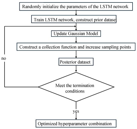
Figure 1. The Flow Chart of Bayes Optimization.

2.1.2. Long Short-Term Memory

Long Short-Term Memory is a specialized type of neural network designed to address the gradient and memory limitations of RNN in sequential data processing. Unlike RNNs, which contain a single Tanh activation structure, LSTM features a more complex four-layer architecture. This structure enhances the global sequence features. Each LSTM unit comprises three gates: input, forget, and output gates, along with a memory cell, as shown in Figure 2.

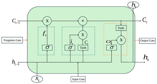
Figure 2. LSTM Unit Structure.

In Figure 2, the Sigmoid activation function $\sigma$ regulates the gating mechanisms, while the Tanh function scales the values within the network. LSTM controls the state of network units through three gates: the forget gate, input gate, and output gate. The blue dashed box represents the “gate control unit”, and the orange dashed box represents the “status transmission path”, This mechanism enables adaptive learning of sequential features by filtering out irrelevant information and preserving useful data. Feature extraction is first performed by the CNN and then passed to the LSTM for processing. The forget gate, activated by the Sigmoid function, determines how much of the previous time step’s state is retained or discarded when updating the current state. The input gate regulates which new information is stored or updated based on activation value $i_t$ and the candidate memory cell state ${\tilde{C}}_t$. The output gate controls which information is transmitted forward by considering the activation output $O_t$ and the memory cell’s output value $h_t$. The specific mathematical formulations at time $t$ are as follows:

$$\left\{\begin{array}{c}{f}_t=\sigma \left({\omega }_f{h}_{t-1}+U_f{x}_t+b_f\right)\\ i_t=\sigma \left({\omega }_f{x}_t+U_i{h}_{t-1}+b_t\right)\\ {\tilde{C}}_t=\mathrm{t}\mathrm{a}\mathrm{n}\mathrm{h}\left(W_c{x}_t+U_c{h}_{t-1}+b_t\right)\\ C_t=i_t\times {\tilde{C}}_t+f_t\times C_{t-1}\\ o_t=\sigma \left({\omega }_o{x}_t+U_o{h}_{t-1}+b_o\right)\\ h_t=o_t\times \mathrm{t}\mathrm{a}\mathrm{n}\mathrm{h}\left(C_t\right)\end{array}\right.$$

(2)

In the equation, $f_t,i_t$, and $o_t$ represent the results of the gate computations. $\sigma$ denotes the Sigmoid activation function, which outputs values of either 0 or 1. The Tanh activation function produces output values ranging from −1 to 1. $\omega$ represents the weight matrix, while $W_c$ is the weight matrix for the candidate values. $h$ is the LSTM output, and $U$ is the weight vector for the input state. $x_t$ is the input at time $t.b_f$ is the bias vector. $C_t$ is the memory cell state, and ${\tilde{C}}_t$ denotes the candidate state.

2.1.3. Self-Attention Mechanism

The self-Attention mechanism is a technique in deep learning used to model features of sequential data. It adaptively assigns weights by focusing on the relationships between information at different positions within the input sequence, thus capturing global dependencies in the sequence data.

Assuming the input is a sequence $X=\left[{\mathit{x}}_1,{\mathit{x}}_2,\dots ,{\mathit{x}}_n\right]$, where each element ${\mathit{x}}_i\in R^d$ has a length of $n$ and a dimensionality of $d$. The selfAttention mechanism captures global dependencies in the sequence data by performing linear transformations, calculating attention weights, and computing weighted value vectors.

(1)

Linear Transformation

For each input ${\mathit{x}}_i$, three different linear transformations are applied to generate the query, key, and value vectors:

$$\left\{\begin{array}{l}\mathit{Q}=\mathit{X}{\mathit{W}}_Q\\ \mathit{K}=\mathit{X}{\mathit{W}}_K\\ \mathit{V}=\mathit{X}{\mathit{W}}_V\end{array}\right.$$

(3)

In the equation, ${\mathit{W}}_Q\in {\mathbb{R}}^{d\times d_k},{\mathit{W}}_K\in {\mathbb{R}}^{d\times d_k}$ and ${\mathit{W}}_V\in {\mathbb{R}}^{d\times d_k}$ are learnable weight matrices, and $d_k$ is the dimensionality of the key and query vectors.

(2)

Calculate Attention Weights

The similarity between the query and key vectors is computed using the dot product, followed by normalization:

$$A=\mathrm{s}\mathrm{o}\mathrm{f}\mathrm{t}\mathrm{m}\mathrm{a}\mathrm{x}\left({\displaystyle \frac{\mathit{Q}{\mathit{K}}^T}{\sqrt{d_k}}}\right)$$

(4)

In the equation, $\sqrt{d_k}$ is the scaling factor, used to prevent excessively large dot product values from affecting the stability of the gradients. The Softmax function is then applied to normalize the weights to the range [0, 1].

(3)

Calculate Weighted Value Vectors

The attention weight matrix $A$ is used to compute a weighted sum of the value vectors $V$, generating the final output.

$$W_o=AV$$

(5)

2.1.4. Classification Evaluation Metrics

A Confusion Matrix is a tabular representation used to evaluate the performance of a classification model, particularly for binary and multiclass tasks. In this article, the confusion matrix is used to compare the predicted values with the actual values for four types of transmission line faults, providing a detailed display of the distribution of correct and incorrect classification results.

For a binary classification task, the confusion matrix is shown in Table 1.

Table 1. Form of confusion matrix for binary classification tasks.

	Predicted as Positive Class	Predicted as Negative Class
Actually classified as positive	True Positive (TP)	False Negative (FN)
Actually classified as negative	False Positive (FP)	True Negative (TN)

TP (True Positive): The actual positive class, predicted as positive. FN (False Negative): The actual positive class, predicted as negative. FP (False Positive): The actual negative class, predicted as positive. TN (True Negative): The actual negative class, predicted as negative.

For evaluating the training results of this algorithm, both the Polygon Area Metric (PAM) and the Receiver Operating Characteristic (ROC) curve are utilized. The PAM is a comprehensive performance evaluation method that normalizes multiple key indicators of the classification model (such as accuracy, sensitivity, specificity, etc.) into a single polygon area value, providing an intuitive quantification of the model’s overall performance. Compared to traditional single metrics like accuracy and Area Under roc Curve (AUC), PAM offers a multidimensional evaluation framework that comprehensively reflects the model’s performance across various aspects.

In PAM, the following six classification performance metrics are selected as the vertices of the polygon:

Classification Accuracy (CA):

$$CA={\displaystyle \frac{TP+TN}{TP+TN+FP+FN}}$$

(6)

Reflects the proportion of samples that the model predicts correctly out of all the samples that participate in the prediction.

Sensitivity (SE):

$$SE={\displaystyle \frac{TP}{TP+FN}}$$

(7)

The model’s sensitivity to positive class samples, the higher the sensitivity, the lower the probability of missed detection.

Specificity (SP):

$$SP={\displaystyle \frac{TN}{TN+FP}}$$

(8)

It refers to the difference in features between negative and positive class samples, and these feature differences are used for judgment. The higher the specificity, the more accurate the judgment. Area Under the Curve (AUC): AUC measures the area under the ROC curve, indicating the classification model’s ability to differentiate between positive and negative classes.

Kappa Coefficient (K):

$$K={\displaystyle \frac{TP}{TP+FP+FN}}$$

(9)

Compares the model’s predictive performance against random classification.

F1 Score (FM):

$$\mathrm{P}\mathrm{r}={\displaystyle \frac{TP}{TP+FP}}$$

(10)

$$\mathrm{R}\mathrm{e}={\displaystyle \frac{TP}{TP+FN}}$$

(11)

$$FM={\displaystyle \frac{2\mathrm{P}\mathrm{r}\cdot \mathrm{R}\mathrm{e}}{\mathrm{P}\mathrm{r}+\mathrm{R}\mathrm{e}}}$$

(12)

The ROC curve is a visual tool for evaluating a classification model’s performance. In binary classification tasks, the model outputs a probability score (between 0 and 1) representing the likelihood of a sample belonging to the positive class. The classification threshold serves as the decision boundary for converting this probability into the final classification result. By adjusting the threshold, one can observe changes in the model’s ability to distinguish between positive and negative samples. The ROC curve illustrates the relationship between the true positive rate (TPR) and false positive rate (FPR) across different threshold values.

X-axis:

$$FPR={\displaystyle \frac{FP}{FP+TN}}$$

(13)

Represents the proportion of negative samples that are incorrectly classified as positive.

Y-axis:

$$TPR={\displaystyle \frac{TP}{TP+FN}}$$

(14)

Represents the proportion of positive samples that are correctly classified.

In this study, the ROC curve was employed as the core tool for evaluating the performance of classification models, and the AUC metric used to quantitatively analyze the models. By constructing a visual representation in a two-dimensional probability space, the discriminative capability of the classifier at different decision thresholds was systematically. The experimental results show that the AUC value, as a comprehensive evaluation index of the model’s distinguishing ability, has a strictly positive correlation with the performance of classifier. Specifically, the greater the degree of deviation of the ROC curve from the random classification baseline (i.e., the diagonal line $\mathrm{y}=\mathrm{x}$) and the more significant the trend of the curve converging to the left-upper quadrant of the coordinate space, the better the classification accuracy and specificity of the.

This geometric characteristic has a strict mathematical correspondence with the discriminative ability of the model in the feature space, providing reliable theoretical basis and intuitive visual criteria for the performance of the classifier.

2.2. Fault Classification Process

The model proposed in this article integrates Bayes inference, LSTM, and self-Attention mechanism to classify transmission line faults. By preserving the original fault signals, it avoids human intervention during data preprocessing thereby maintaining data quality. The network architecture is shown in Figure 3.

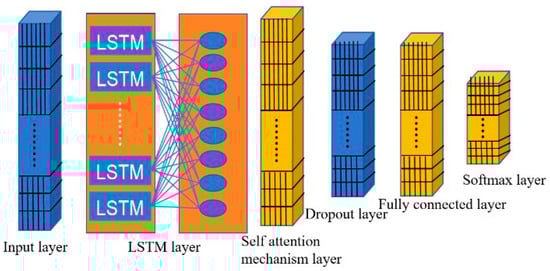
Figure 3. Bayes LSTM Attention Network Model.

In Figure 3, the fault classification model follows a sequential structure, consisting of an input layer, an LSTM layer, a self-Attention mechanism layer, a Dropout layer, a fully connected layer, and a softmax layer. The final output is generated through the cross-entropy function softmax.

The input layer of the model receives sequential data from 12 time steps. The LSTM layer consisting of 17 hidden units with a bias term of 17, captures temporal features and outputs both the hidden state (HiddenState) and cell state (CellState).

A rectified linear unit (ReLU) activation function is then applied to the LSTM output to introduce nonlinearity and enhance the model’s representational capability. To further capture dependencies across different positions in the sequence, a self-Attention mechanism is incorporated via the self-attention layer. This layer uses weight matrices $W_Q,W_K$, and $W_V$ to compute a weighted sum of the LSTM outputs, generating an attention map. To avoid overfitting, a Dropout layer with a dropout rate set to $1\mathrm{\%}$ is introduced. The fully connected layer integrates the extracted features, producing an output dimension of 4. Finally, the softmax layer computes the classification probabilities, generating a probability distribution over 4 classes, while the cross-entropy loss function quantifies the classification error. By combining time-series modelling, contextual dependency capture, and feature enhancement, the proposed architecture effectively addresses the transmission line fault classification problem.

During training, the loss function continuously adjusts the weights and biases to minimize the difference between the output and the desired value. This paper uses the categorical cross-entropy loss function, which is computed as follows:

$$L=-{\displaystyle \frac{1}{n}}\sum _n^{i=1} x_i\times \mathrm{l}\mathrm{o}\mathrm{g}{x}_i$$

(15)

In the equation, L is the loss function, $\hat{x}=\left\{x_1,x_2,\dots ,x_n\right\}$ is the predicted value, and $x=\left\{x_1,x_2,\dots ,x_n\right\}$ is the true value.

3. Results

3.1. Input Data and Parameter Settings

In this paper, the dataset consists of a total of 357 samples (249 samples for the training set and 108 samples for the testing set), with a total of 12 input features. Features 1 and 2 reflect the system’s baseline operating conditions, features 3 to 6 represent steady-state measurements such as phase currents and power, features 7 and 8 indicate quality metrics like harmonics and power factor, and features 9 to 12 represent high-frequency transients and sequence components, our preprocessing process includes the following steps: handling missing values, handling outliers, data normalization, data reconstruction, and dataset partitioning, the LSTM network is applied to rearrange the original two-dimensional sample data into four-dimensional data based on the given parameters to meet the input format requirements of the LSTM network and generate pseudo-time series. The default time step and the number of channels are both set to 1. In terms of model parameters, the number of LSTM hidden layer nodes is selected as 17 based on the Bayesian optimization. The initial learning rate is set to 0.0098, the L2 regularization coefficient to 0.0045, and the number of iterations to 500. The backpropagation algorithm is used for fault classification training, with the Adam optimizer iteratively updating the model parameters at each layer to obtain the final Bayes–LSTM–Attention-based fault classification model for three-phase transmission lines.

3.2. Classification Result Analysis

Figure 4 illustrates the relationship between training accuracy, loss function, and the number of iterations for fault diagnosis using the Bayes–LSTM–Attention model.

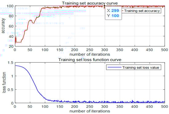
Figure 4. Training set accuracy and loss function curve.

The accuracy and loss function curves show that the model converges rapidly within the first 50 iterations. The loss function decreases quickly, while accuracy increases sharply, indicating that the model effectively captures most line fault features early in training. After approximately 100 iterations, both accuracy and loss stabilize, reaching a steady state. The accuracy remains above 98%, and the loss value approaches 0.1, demonstrating a strong fit to the fault data.

The transmission line fault classification in this paper involves four categories, forming a four-class classification task. The four types of faults selected for this study are the most common and significant fault types in three-phase transmission lines of the power system. They are single-phase grounding faults, double-phase short-circuit faults, double-phase grounding faults, and three-phase short-circuit faults. These four types of faults together constitute a complete fault set that includes both symmetrical and asymmetrical faults, as well as short-circuit and disconnection faults. It can comprehensively test the classification performance and generalization ability of the proposed Bayes LSTM Attention model under different fault mechanisms and electrical characteristics (such as zero sequence, negative sequence components, and transient characteristics), ensuring the engineering practicality and academic completeness of the research results. Table 2 shows the fault data set class distribution, and the dataset ensures that the proportion differences among categories are less than 1% through ‘stratified sampling’, with no significant class imbalance issues. Two 4 × 4 confusion matrices are generated for different categories, as shown in Figure 5 and Figure 6, corresponding to the training and test sets, respectively. Table 3 below presents the prediction results for both the training and test sets. Figure 5 shows the confusion matrix of the model on the test set, and combined with Table 3, the model achieves an overall accuracy of 95.9% on the training set, indicating a good fit to the training data. It can be observed that misclassifications are mainly concentrated in categories 2 and 4. Analysing Figure 6, combined with Table 3, the overall accuracy of the model on the test set is 95.4%, which is slightly lower than the accuracy on the training set, indicating a mild overfitting tendency of the model on the test set. Misclassifications still occur in categories 1, 2, and 4. However, the classification accuracy of category 3 has significantly declined. Despite this, the overall accuracy remains quite high, reflecting the model’s strong generalization ability across different categories of line faults. The prediction errors in the confusion matrix of the test set shown in Figure 6 are mainly due to the inherent similarity of electrical characteristics between different fault types, which poses a fundamental challenge to the classification task. We observed that the prediction errors occurred between type 2 (phase to phase short circuit) and type 4 (disconnection fault). From the perspective of power system principles, the electrical characteristics of these two types of faults are highly similar under certain operating conditions. For example, certain asymmetric disconnection faults can lead to unbalanced line currents, and their waveform characteristics are very similar to phase short-circuit faults, making it difficult for the model to distinguish them absolutely.

Table 2. Fault Data Set Class Distribution.

Fault Category	Number of Training Samples	Number of Testing Samples	Total Number of Samples	Proportion
Type 1	62	27	89	24.93%
Type 2	62	27	89	24.93%
Type 3	62	27	89	24.93%
Type 4	63	27	90	25.21%
Total	249	108	357	100%

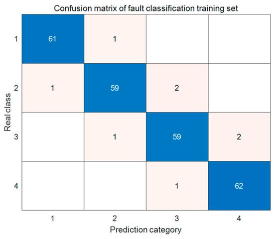
Figure 5. Confusion Matrix of Training Set.

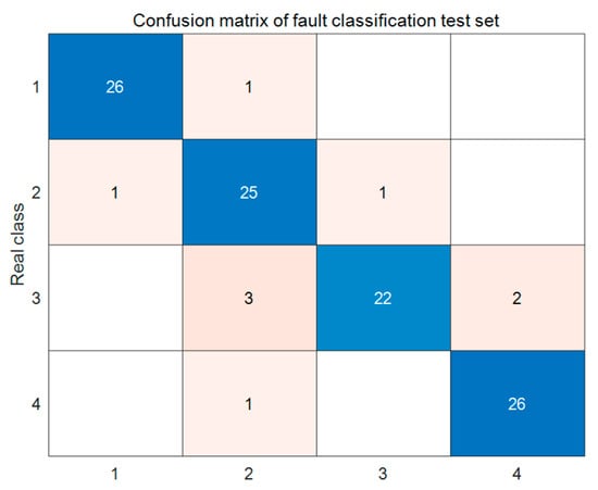
Figure 6. Test set confusion matrix.

Table 3. Training and test set prediction results.

Sample Category	Prediction Correct	Forecast Error	Accuracy
Training set	239	10	95.9%
Test set	103	5	95.4%

Figure 7 shows the polygon area evaluation metric for the fault classification test set predictions, while Figure 8 presents the ROC curve for the test set. The dashed line represents the ideal classification boundary, and the shaded area represents the performance range of the model on the test set. The CA value is 0.954, indicating that the model achieves a 95.4% correct classification rate on the test set, suggesting that the model can correctly predict the sample categories in most cases. The Kappa coefficient is 0.93, demonstrating a very high consistency between the predicted and actual results, showing strong discriminative ability for faults in the test set. Additionally, the F1 Score (FM) value is 0.96, indicating that the model performs well in both precision and recall, maintaining high precision while achieving a high recall of samples without significant bias. The AUC value is 0.99, indicating that the model has excellent discriminative ability and can effectively distinguish between different line fault samples. The AUC value close to 1 reflects the model’s excellent stability in response to changes in the classification threshold, maintaining a high correct classification rate even with varying thresholds. Overall, these evaluation metrics are excellent, with the PAM value at 0.92, indicating that the Bayes–LSTM–Attention model offers balanced and robust classification performance for line faults.

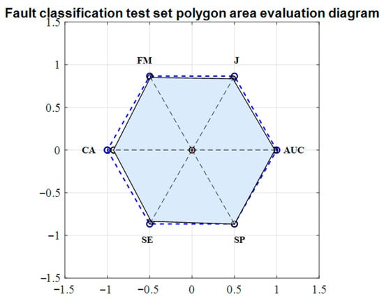
Figure 7. Fault classification test set polygon area evaluation diagram.

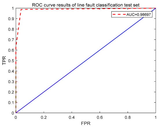
Figure 8. ROC curve results of line fault classification test set.

The ROC curve is almost tightly aligned with the top-left corner, indicating that the model maintains high fault discrimination ability across different thresholds. The AUC value close to 1 shows that even when certain fault states in the power system change, the model can still effectively identify these fault types. The efficient fault identification ensures the safety of the power system’s operation, also demonstrating the superiority of this method in handling similar fault classification tasks.

As shown in Figure 9 and Figure 10, corresponding to the training set and the test set, respectively. Figure 10 shows the prediction results of the model on the test set, with an overall accuracy of 94.4444% on the test set, indicating the model fits the data well. Analyzing Figure 9, the accuracy of the model on the training set was 93.1727% slightly lower than the accuracy on the test set, indicating that the model has a slight tendency of overfitting on the test set. Nevertheless, the overall accuracy is still high, reflecting the strong generalization ability of the model in different types of line faults.

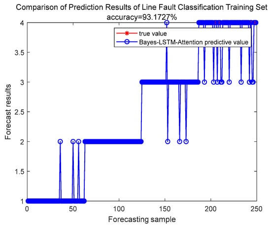
Figure 9. Comparison of Prediction Results of Line Fault Classification Training Set.

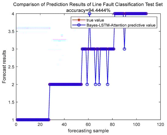
Figure 10. Comparison of Prediction Results of Line Fault Classification Test Set.

4. Discussion

This paper proposes a fault classification model for three-phase transmission lines that combines Bayesian optimization, self-Attention mechanisms, and LSTM networks. Specifically, using a real-world three-phase line fault dataset, Bayesian optimization is used to determine essential hyperparameters for building the LSTM model, such as the number of hidden layer nodes, learning rate, and regularization coefficient. The input data is transformed and trained with the LSTM network, and the results are evaluated using confusion matrices. Evaluation metrics are calculated using the polygon area evaluation method, leading to the following conclusions:

(1)

By learning 12 distinct features of fault samples through the LSTM network, the proposed Bayes–LSTM–Attention model demonstrates superior accuracy in fault classification, with a prediction accuracy of 95.3% on the test set, demonstrating high classification precision and overall effectiveness.

(2)

A comparison of the true and predicted values for both the training and test sets reveals similar accuracy, indicating that the model exhibits strong generalization ability for various line fault types. Additionally, evaluation metrics generated using the polygon area method demonstrate the model’s high precision and stability in fault classification for transmission lines.

(3)

By introducing the self-attention mechanism, the model is able to adaptively focus on the key information in the fault sequence, enhancing its ability to global dependencies. Combined with the analysis results of the Polygon Area Metric (PAM) and the ROC curve, the model exhibits high classification stability and robustness different thresholds, and can effectively respond to the complex and changeable fault scenarios in power systems, providing reliable technical support for practical applications.

This method provides effective support for the operation and maintenance of transmission lines, and the deep learning-based model has the potential to adapt to various dynamic scenarios in practical applications. Future research could focus on further optimizing the model structure or incorporating additional fault features to improve classification performance and address more complex scenarios.

References

- Liang, Z.R.; Niu, S.S.; Jin, N. Current situation and development trend of parameter measurement of AC lines. Autom. Electr. Power Syst. 2017, 41, 181–191. [Google Scholar]
- Wang, Y.T.; Zhang, B.H.; Fan, X.K. A rapid protection scheme for overhead lines in flexible DC power grid. Autom. Electr. Power Syst. 2016, 40, 13–19. [Google Scholar]
- Yang, J.; Luo, G.; He, Z. A fault classification method for high-voltage transmission lines based on wavelet entropy and support vector machine. Power Grid Technol. 2007, 23, 22–26+32. [Google Scholar]
- Wu, X.; Cao, W.; Wang, D.; Ding, M. A fault diagnosis method for transmission lines on multi-supportvect or machine models. High Volt. Technol. 2020, 46, 957–963. [Google Scholar] [CrossRef]
- Zhao, W. Research on Fault Classification and Fault lo Cation of MMC-HVDC Direct Current Line Based on VWAA-SVM. Master’s Thesis, Lanzhou University of Technology, Lanzhou, China, 2023. [Google Scholar] [CrossRef]
- Zhao, R. Fault Feature Extraction and Diagnosis of Transmission Line Based on Improved HHO Optimization VMD-SVM model. Master’s Thesis, Lia University of Technology, Fuxin, China, 2023. [Google Scholar] [CrossRef]
- Song, J. Prediction Method for Ice Accretion and Galloping of Transmission Lines Based on FEM and Improved PSO-SVM Algorithm. Master’s Thesis, Three Gorges University, Yichang, China, 2024. [Google Scholar]
- Wei, W.; Gao, C.; Song, M.; Ming, H. Power line fault detection classification system based on HHO-SVM. Integr. Smart Energy 2023, 45, 1–8. [Google Scholar]
- Zou, H.; Song, J.; Liu, Y.; Duan, Z.; Zhang, X.; Song, L. A prediction mode l of transmission line icing galloping based on O-SVM algorithm. J. Vib. Shock 2023, 42, 280–286. [Google Scholar] [CrossRef]
- Zhang, S.; Guo, Y.; Zhang, X.; Ning, X.; Yin, C. Research on fault diagnosis of power lines on SVM-RF. Shandong Electr. Power Technol. 2022, 49, 36–43. [Google Scholar]
- Wei, J. Fault Diagnosis and Location of Active Distribution Networks Based on SVM. Master’s Thesis, North China Electric Power University, Beijing, China, 2021. [Google Scholar] [CrossRef]
- Ray, P.; Mishra, D.P.; Dey, K.; Mishra, P. Fault Detection and Classification of a Transmission Line Using Discrete Wavelet Transform & Artificial Neural Network. In Proceedings of the 2017 International Conference on Information Technology (ICIT), Bhubaneswar, India, 27–29 December 2017; pp. 178–183. [Google Scholar]
- Yang, S.Z.; Wang, X.; Zhang, J.K.; Rao, H.; Xu, S.; Huang, R.; Wen, J. Fault detection method for overhead flexible DC grid based on artificial neural. Proc. Chin. Soc. Electr. Eng. 2019, 39, 4416–4430. [Google Scholar] [CrossRef]
- Kumari, S.; Mishra, A.; Singhal, A.; Dahiya, V.; Gupta, M.; Gawre, S.K. Fault Detection in Transmission Line Using ANN. In Proceedings of the 2023 IEEE International Students’ Conference on Electrical, Electronics and Computer Science (SCEECS), Bhopal, India, 18–19 February 2023; pp. 1–5. [Google Scholar] [CrossRef]
- Leh, N.A.M.; Zain, F.M.; Muhammad, Z.; Hamid, S.A.; Rosli, A.D. Fault Detection Method Using ANN for Power Transmission Line. In Proceedings of the 2020 10th IEEE International Conference on Control System, Computing and Engineering (ICCS CE), Penang, Malaysia, 21–22 August 2020; pp. 79–84. [Google Scholar] [CrossRef]
- Dong, S.; Lu, X.; Sun, H.; Ye, Q. Research on fault location of power lines on signal analysis technol ogy and artificial intelligence algorithm. Energy Environ. Prot. 2022, 44, 35–40. [Google Scholar] [CrossRef]
- Chen, X.; Sun, L.; Li, Y.; Li, B. A Double-ended Transmission Line Non-synchronous Fault Location Algorithm Based on Artifi cial Neural Network and Migration. Power Grid Technol. 2023, 47, 5169–5181. [Google Scholar] [CrossRef]
- Sun, X.; Qin, L.; Liu, D. A Comprehensive Fault Identification Method for Transmission Lines Base d on GMAPM and SOM-LVQ-ANN. J. Wuhan Univ. Technol. (Eng. Ed.) 2019, 52, 1079–1090+1105. [Google Scholar] [CrossRef]
- Zhang, Y.; Li, P.; Xu, D. A method for fault location of transmission lines based on neural network. Electr. Eng. Technol. 2004, 2, 50–53+83. [Google Scholar]
- Yang, J. Research on a New Method of Fault Location in Transmission Lines Based on Artificial Neural Networks. Master’s Thesis, Sich University, Chengdu, China, 2004. [Google Scholar]
- Shu, H.; Wu, Q.; Zhang, G.; Sun, S.; Liu, K. single-ended traveling wave fault location method based on neural network. Proc. Chin. Soc. Electr. Eng. 2011, 31, 85–92. [Google Scholar] [CrossRef]
- Devi, M.M.; Sharma, M.; Ganguly, A. Detection and Classification of Transmission Line Faults using LSTM Algorithm. In Proceedings of the 2023 IEEE 2nd International Conference on Industrial Electronics: Developments & Applications (ICIDeA), Imphal, India, 29–30 September 2023; pp. 146–151. [Google Scholar] [CrossRef]
- Rajashekar, J.; Yadav, A. Transmission lines Fault Detection and Classification Using Deep Learning Neural Network. In Proceedings of the 2022 Second International Conference on Advances in Electrical, Computing, Communication and Sustainable Technologies (ICAECT), Bhilai, India, 21–22 April 2022; pp. 1–6. [Google Scholar] [CrossRef]
- Feng, Y.; Jia, H.; Yang, Z.; Geng, W.; Wang, J. Research on fault diagnosis method of transmission line on CNN-LSTM. Power Grid Clean Energy 2023, 39, 59–65. [Google Scholar]
- Song, K.; Wu, H.; Chen, W. A method for identifying fault lines in AC and DC power grids based CNN-LS TM networks. J. Sichuan Univ. Sci. Eng. (Nat. Sci. Ed.) 2024, 37, 50–58. [Google Scholar]
- Du, Y. Research on Guided Search of High-Voltage Line Cascading Failure Based on GCN-LSTM. Master’s Thesis, North China Electric Power University, Beijing, China, 2024. [Google Scholar] [CrossRef]
- Wei, R.; Chen, S.; Bi, G.; Deng, X.; Niu, Y.; Yao, H. Research on fault location of UHV line based on hybrid LSTM deep learning. Electr. Power Sci. Eng. 2023, 39, 1–10. [Google Scholar]
- Wu, J.; Zhang, Y.; Li, S.; Wang, F. Research on intelligent diagnosis method of line fault based on LSTM. Large Mot. Technol. 2023, S2, 62–67. [Google Scholar]
- Chen, C.; Chen, S.; Bi, G.; Gao, J.; Zhao, X.; Li, L. Fault diagnosis of weak receiving-end DC transmission system on par. Electr. Mach. Control Appl. 2022, 6, 49. [Google Scholar]
Disclaimer/Publisher’s Note: The statements, opinions and data contained in all publications are solely those of the individual author(s) and contributor(s) and not of MDPI and/or the editor(s). MDPI and/or the editor(s) disclaim responsibility for any injury to people or property resulting from any ideas, methods, instructions or products referred to in the content. |
© 2025 by the authors. Licensee MDPI, Basel, Switzerland. This article is an open access article distributed under the terms and conditions of the Creative Commons Attribution (CC BY) license (https://creativecommons.org/licenses/by/4.0/).