Power Quality Data Augmentation and Processing Method for Distribution Terminals Considering High-Frequency Sampling

Abstract

The safe and stable operation of distribution networks relies on the real-time monitoring, analysis, and feedback of power quality data. However, with the continuous advancement of distribution network construction, the number of distributed power electronic devices has increased significantly, leading to frequent power quality issues such as voltage fluctuations, harmonic pollution, and three-phase unbalance in distribution terminals. Therefore, the augmentation and processing of power quality data have become crucial for ensuring the stable operation of distribution networks. Traditional methods for augmenting and processing power quality data fail to consider the differentiated characteristics of burrs in signal sequences and neglect the comprehensive consideration of both time-domain and frequency-domain features in disturbance identification. This results in the distortion of high-frequency fault information, and insufficient robustness and accuracy in identifying Power Quality Disturbance (PQD) against the complex noise background of distribution networks. In response to these issues, we propose a power quality data augmentation and processing method for distribution terminals considering high-frequency sampling. Firstly, a burr removal method of the sampling waveform based on a high-frequency filter operator is proposed. By comprehensively considering the characteristics of concavity and convexity in both burr and normal waveforms, a high-frequency filtering operator is introduced. Additional constraints and parameters are applied to suppress sequences with burr characteristics, thereby accurately eliminating burrs while preserving the key features of valid information. This approach avoids distortion of high-frequency fault information after filtering, which supports subsequent PQD identification. Secondly, a PQD identification method based on a dual-channel time–frequency feature fusion network is proposed. The PQD signals undergo an S-transform and period reconfiguration to construct matrix image features in the time–frequency domain. Finally, these features are input into a Convolutional Neural Network (CNN) and a Transformer encoder to extract highly coupled global features, which are then fused through a cross-attention mechanism. The identification results of PQD are output through a classification layer, thereby enhancing the robustness and accuracy of disturbance identification against the complex noise background of distribution networks. Simulation results demonstrate that the proposed algorithm achieves optimal burr removal and disturbance identification accuracy.

1. Introduction

With the growing penetration and scale of renewable energy in power systems, the distribution network has changed from the traditional one-way single-source mode to the multi-direction multi-source mode. Numerous distributed generation units and nonlinear power electronic devices have been incorporated into the distribution grid, leading to power quality issues, including voltage fluctuations, harmonic distortion, and three-phase imbalance. These issues are becoming increasingly prominent, posing severe challenges to power supply quality [1,2]. To maintain the proper functioning of power equipment and prevent system faults from spreading, real-time monitoring of power quality data is essential for promptly analyzing and addressing anomalies. This helps minimize power equipment damage and financial losses while enhancing the power system’s operational efficiency. However, electromagnetic interference within distribution terminals and the weak noise resistance of microprocessor-embedded chips often cause power quality data waveforms to exhibit burrs, distortion, and disturbances. This makes it more difficult to extract and identify fault features [3,4]. Therefore, it is urgent to investigate power quality data enhancement and processing techniques for distribution terminals under the complex distribution network noise environment. These studies enhance data feature extraction, improve disturbance identification robustness and accuracy, and strongly support power quality monitoring and fault warning.

Due to electromagnetic interference and complex noise in the distribution terminal and microprocessor during high-frequency acquisition, the collected electrical waveform will appear to have a burr, which increases the difficulty of power quality detection and analysis [5]. In traditional research, low-pass filtering or wavelet transform is used to remove the tip burr component and clean the data. A method for mitigating large burr signals was proposed, which is derived from the established theory of nonlinear systems and the burr threshold boundary [6]. Under the condition of same hardware, the influence of the burr phenomenon can be reduced by combining the burr jitter of sufficient amplitude with low-pass filtering. In [7], Tian et al. carried out wavelet domain filtering and threshold processing on the bus load data based on the wavelet threshold denoising method to remove burr in the waveform. However, when processing high-frequency signal sequences, the traditional low-pass filtering method may cause signal distortion or degradation. This is particularly problematic for high-frequency components containing key features of power quality, as it is often difficult to balance the contradiction between denoising and retaining useful information, which affects the subsequent analysis of power quality data.

Renewable energy power systems and nonlinear load grid connections can lead to Power Quality Disturbance (PQD), resulting in signal degradation and waveform distortion. These issues significantly impact the stable and secure operation of precision computers and microprocessors within the distribution network, potentially leading to anomalies or severe accidents [8]. Consequently, accurately identifying and classifying PQD is essential for enhancing power supply quality, monitoring power equipment conditions, and preventing grid faults. Traditional PQD classification methods rely on techniques such as Short-Time Fourier Transform (STFT), S-transform (ST), and wavelet transform for feature extraction. These manually selected features serve as classifier inputs, mapping extracted features to disturbance categories [9,10]. In [11], Tang et al. introduced a PQD detection and classification approach utilizing ST and a kernel Support Vector Machine (SVM) to mitigate the signal distortion caused by nonlinear load integration into the distribution network. By optimizing window parameters and employing multi-feature classification with kernel functions, effective PQD classification under varying noise levels was achieved. Similarly, an improved wavelet transform-based PQD identification method was proposed in [12]. This approach leveraged a two-tree wavelet transform to extract complex disturbance features and employed a directed acyclic graph SVM for PQD classification. Additionally, SVM parameters were fine-tuned using the locust optimization algorithm, improving both classification accuracy and processing speed. In [13], Abdelsalam et al. introduced a PQD identification method that uses a Kalman filter for automatic detection and burr removal. It then classifies disturbances based on three factors: the three consecutive maximum values of instantaneous total harmonic distortion, the standard deviation, and the energy difference between the distorted signal and its fundamental frequency. In [14], Zhao et al. combined time–frequency domain multi-features with a decision tree for disturbance identification. It uses energy spectrum features from wavelet transform and other time–frequency features from S-transform to create identification rules. However, as noise complexity increases within distribution networks, traditional methods that rely on statistical analyses and experience-based feature extractions become less effective. Moreover, conventional classifiers struggle with generalization and slow processing speeds when handling large-scale datasets. Deep learning, with its multi-layered structure, offers robust nonlinear feature extraction capabilities. Architectures such as Convolutional Neural Networks (CNN) and autoencoders enable autonomous learning from extensive PQD datasets. These models convert one-dimensional PQD signal sequences into two-dimensional representations, allowing image-processing techniques to directly extract features, recognize disturbance patterns, and classify PQD signals [15]. In [16], Cui et al. proposed a CNN-based method for multi-class PQD classification, where a one-dimensional feature matrix is extracted using ST. After optimizing the contour parameters to generate a two-dimensional image, it is then input into the CNN for training to complete the PQD classification task under different interference conditions. An automatic identification and classification method of PQD based on deep learning was designed. Multidimensional spectral characteristics of the fractional domain were extracted through spatial Fourier transform. These characteristics were then converted into spatial feature maps [17]. The multi-inputs were sent to a deep spectrum convolution fusion network for multidimensional feature fusion and PQD classification. This can improve the detection and anti-noise ability of complex PQD signals. However, the large number of network parameters, the high computational complexity, the inability to parallelize calculation, and the long-distance dependence of these structures limit their application in large-scale power quality data processing.

Being a highly capable deep learning model, long-range dependencies and global context in time series data are effectively captured by the Transformer via its self-attention mechanism. This addresses the limitation of neural networks, which struggle to perform parallel and balanced computation simultaneously [18]. In [19], Yoon et al. introduced a deep PQD identification technique based on the Transformer. By segmenting voltage signal inputs and embedding them into Transformer encoders, the model accurately classifies PQD types and locations under different fault conditions using a multi-head attention mechanism and multi-layer perceptron. Similarly, an end-to-end disturbance identification framework integrating deep CNN and the Transformer was proposed in [20]. This approach employs a deep CNN for one-dimensional feature extraction, while a Transformer encoder and attention mechanism facilitate sequence-based autonomous learning and feature fusion, enhancing the speed and accuracy of fault detection and prediction. In [21], Chen et al. constructed an optimization algorithm based on the STFT and CNN. By converting signal samples into time–frequency matrices as inputs for the CNN, the algorithm leverages the powerful two-dimensional data processing capability of CNNs to achieve more efficient interference recognition. In [22], Zhou et al. adopted a dual-branch structure combining CNN and Long Short-Term Memory (LSTM) to process raw time series data and wavelet transform coefficients. They used the Continuous Wavelet Transform (CWT) to extract time–frequency features and employed an LSTM layer with a self-attention mechanism to capture temporal dynamics. Despite its effectiveness in identifying PQD, the CNN models typically process only single-mode sequence features, overlooking the interrelation between time and frequency domains as well as the complementary nature of multi-dimensional information. Consequently, under complex noise conditions in the distribution network, achieving precise signal characterization remains challenging, ultimately affecting detection performance.

In summary, the following challenges remain in power quality data processing. Firstly, due to the electromagnetic interference inside the distribution terminal and the weak anti-noise ability of the chip embedded in the microprocessor, the collected signal sequence appears as a burr. The traditional low-pass filtering method easily causes high-frequency information distortion, affecting the subsequent analysis of power quality data. Secondly, traditional PQD identification methods are often based on single-frequency domain signal processing or deep learning algorithms. These methods ignore the comprehensive consideration of the dual characteristics of the time domain and frequency domain, and are unable to accurately capture the long-distance dependence between different sequences. Additionally, the large number of network parameters makes parallel computation impossible, resulting in the insufficient robustness and accuracy of PQD identification in the complex noise environment in the distribution network.

Therefore, in order to solve the above problems, we propose a power quality data augmentation and processing method for distribution terminals considering high-frequency sampling to improve the robustness and accuracy of PQD identification in complex noise environments. Firstly, a burr removal method based on a high-frequency filter operator is proposed to address the burr caused by electromagnetic interference, noise, and related faults. Only power quality sampling sequences that exhibit burr characteristics are suppressed, while key information from the normal bumps of the original waveform is preserved through additional constraints. The filtered signal sequence is then analyzed and processed in the time–frequency domain. Using S-transform and signal period reconstruction, the original one-dimensional signal is transformed into a two-dimensional matrix image, enabling the extraction of multi-modal PQD signal features. A PQD identification approach based on a dual-channel time–frequency feature fusion network is proposed. The time–frequency domain matrix image is simultaneously fed into a CNN and Transformer encoder to extract globally coupled features. A cross-attention mechanism is employed for feature fusion, enhancing features’ representation and ultimately enabling accurate PQD classification. The comparisons between the proposed work and other works from the perspectives of operator complexity, preservation of transients, dual characteristics of time–frequency domains, long-term dependency capture capability, and burr removal without high-frequency information distortion are shown in Table 1. The main contributions of this paper are summarized as follows.

Table 1. The comparisons between the proposed work and other works.

	Operator Complexity	Preservation of Transients	Dual Characteristics of Time–Frequency Domains	Long-Term Dependency Capture Capability	Burr Removal Without High-Frequency Information Distortion
Median filter	Low	×	×	×	√
Top-hat transform	Medium	×	√	√	×
[13]	High	×	×	×	√
[14]	Low	×	√	√	×
[16]	High	×	×	√	×
[17]	High	√	√	×	√
[19]	High	√	×	×	√
[20]	High	×	×	√	√
[21]	High	×	√	√	×
Proposed	High	√	√	√	√

• The burr removal method of sampling waveforms based on high-frequency filter operator: The method uses high-frequency filtering operators and takes into account the small bumps that may appear in normal waveforms. By adding different restrictions or parameters, only the sampled signals that meet the burr characteristics are processed. While eliminating burrs, it can accurately retain the key features of high-frequency information, avoid the distortion of high-frequency fault information after filtering, and improve the data quality of the distribution terminal.
• The PQD identification method based on a dual-channel time–frequency feature fusion network: First, the PQD signal undergoes an S-transform and signal period reconstruction to generate a matrix image, forming the dual-channel time–frequency domain input features. Next, two types of matrix image features are fed into a CNN to extract global time-domain and local frequency-domain features. Additionally, a Transformer encoder captures highly coupled global time–frequency features, while the cross-attention mechanism enhances deep fusion by modeling the long-term dependencies between the sequences. Finally, the classification layer outputs the PQD identification results, improving robustness and accuracy in complex distribution network noise conditions.

2. Burr Removal of Sampling Waveforms Based on High-Frequency Filter Operator

High-frequency acquisition in distribution terminals enables the real-time detection of subtle electricity consumption changes, enhancing monitoring accuracy and fault response speed. It supports grid stability and facilitates rapid fault localization. However, in the process of high-frequency acquisition, the electrical waveform is often accompanied by burrs. These burrs are due to electromagnetic noise artifacts, which affect the accuracy of electrical data. Traditional low-pass filtering or basic wavelet denoising methods often indiscriminately attenuate all high-frequency components, which can potentially distort crucial fault information. Therefore, we propose a burr removal method of sampling waveforms based on high-frequency filter operators, as shown in Figure 1. It leverages specialized high-frequency impulse (${\eta }_1,{\eta }_2$) and oscillation (${\beta }_1,{\beta }_2$) operators. These operators are designed to perform a differentiated morphological analysis. They specifically identify and suppress signal sequences that exhibit distinct ‘burr characteristics’ based on their sharp concavity and convexity patterns. A key innovation lies in incorporating additional constraints and a dynamic limiting parameter, $\lambda$. This allows us to process only those sampled signals that conform to burr characteristics and also exceed a specific amplitude deviation threshold. $\lambda$ is dynamically adjusted based on feedback from PQD identification results. This ensures accurate burr elimination while precisely preserving key high-frequency fault signatures. Therefore, this approach prevents the distortion common in conventional filtering and significantly improves the data quality for subsequent PQD identification.

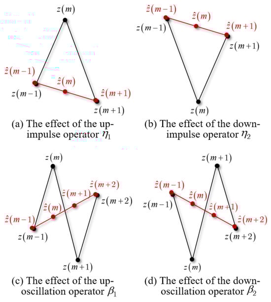
Figure 1. High-frequency filter operator.

2.1. High-Frequency Filter Operator

2.1.1. High-Frequency Shock Filter Operator

The high-frequency impulse filter operator of the distribution terminal acquisition sequence is defined as $\eta$, and it can be subdivided into the up-impulse operator ${\eta }_1$ and the down-impulse operator ${\eta }_2$, as shown in Figure 1.

In Figure 1, $m-1$, m, and $m+1$ represent three adjacent sampling points from $m-1$ to $m+1$. The characteristics of the up-impulse operator ${\eta }_1$ can be expressed as follows:

$${\eta }_1\in \left\{\begin{array}{c}\eta \left(m-1\right)<\eta \left(m\right)\\ \eta \left(m+1\right)<\eta \left(m\right)\end{array}\right.$$

(1)

The characteristics of the down-impulse operator ${\eta }_2$ can be expressed as follows:

$${\eta }_2\in \left\{\begin{array}{c}\eta \left(m-1\right)>\eta \left(m\right)\\ \eta \left(m+1\right)>\eta \left(m\right)\end{array}\right.$$

(2)

Suppose $z\left(m\right)$ is a distribution terminal sampling sequence. $\mathrm{Y}$ represents the up-impulse operator ${\eta }_1$ applied to the distribution terminal sampling sequence. The filtered distribution terminal sampling sequence can be expressed as follows:

$$\widehat{z}\left(m\right)=z\left(m\right)\mathrm{Y}{\eta }_1\left(m\right)$$

(3)

If three adjacent sampling points $z\left(m-1\right)$, $z\left(m\right)$, and $z\left(m+1\right)$ align with the characteristics of the ${\eta }_1$ operator in Equation (1), the signal is filtered by applying Equation (4), which is expressed as follows:

$$\left\{\begin{array}{l}\widehat{z}\left(m-1\right)=z\left(m-1\right)\hfill \\ \widehat{z}\left(m\right)=\left[z\left(m-1\right)+z\left(m+1\right)\right]/2\hfill \\ \widehat{z}\left(m+1\right)=z\left(m+1\right)\hfill \end{array}\right.$$

(4)

If three adjacent sampling points $z\left(m-1\right)$, $z\left(m\right)$, and $z\left(m+1\right)$ do not align with the characteristics of the ${\eta }_1$ operator in Equation (1), the original signal point is directly retained without any filtering operation, which is denoted as follows:

$$\left\{\begin{array}{l}\widehat{z}\left(m-1\right)=z\left(m-1\right)\hfill \\ \widehat{z}\left(m\right)=z\left(m\right)\hfill \\ \widehat{z}\left(m+1\right)=z\left(m+1\right)\hfill \end{array}\right.$$

(5)

Similarly, the down-impulse operator ${\eta }_2$ is applied to the distribution terminal sampling sequence $z\left(m\right)$, and the filtered distribution terminal sampling sequence is obtained, which can be expressed as follows:

$$\widehat{z}\left(m\right)=z\left(m\right)\mathrm{Y}{\eta }_2\left(m\right)$$

(6)

When the down-impulse operator ${\eta }_2$ is applied to the distribution terminal sampling sequence $z\left(m\right)$, if $z\left(m-1\right)$, $z\left(m\right)$, and $z\left(m+1\right)$ align with the characteristics of operator ${\eta }_2$, the calculation is made according to Equation (4). If $z\left(m-1\right)$, $z\left(m\right)$, and $z\left(m+1\right)$ do not align with the characteristics of the ${\eta }_2$ operator, they are calculated according to Equation (5).

In the actual burr removal from the sampling waveform, the operator ${\eta }_1$ and the operator ${\eta }_2$ are often combined to apply to the distribution terminal sampling sequence $z\left(m\right)$, aiming to filter out the high-frequency burrs in the distribution terminal sampling sequence, which can be expressed as follows:

$$\widehat{z}\left(m\right)=z\left(m\right)\mathrm{Y}\left[{\eta }_1\left(m\right)+{\eta }_2\left(m\right)\right]$$

(7)

The combination of the operator ${\eta }_1$ and the operator ${\eta }_2$ on the distribution terminal sampling sequence is described as follows. If $z\left(m-1\right)$, $z\left(m\right)$, and $z\left(m+1\right)$ align with the characteristics of the ${\eta }_1$ or ${\eta }_2$ operators, they are calculated according to Equation (4). If $z\left(m-1\right)$, $z\left(m\right)$ and $z\left(m+1\right)$ do not align with the characteristics of either the ${\eta }_1$ or ${\eta }_2$ operators, they are calculated according to Equation (5).

2.1.2. High-Frequency Oscillation Filter Operator

The high-frequency oscillation filter operator of the distribution terminal acquisition sequence is defined as $\beta$, and it can be subdivided into the up-oscillation operator ${\beta }_1$ and the down-oscillation operator ${\beta }_2$, as shown in Figure 1.

According to the morphological characteristics of high-frequency interference in distribution terminals that need to be filtered out, the characteristics of up-oscillation operator ${\beta }_1$ can be expressed as follows:

$${\beta }_1\in \left\{\begin{array}{l}\beta \left(m-1\right)<\beta \left(m\right)\hfill \\ \beta \left(m-1\right)>\beta \left(m+1\right)\hfill \\ \beta \left(m+2\right)<\beta \left(m\right)\hfill \\ \beta \left(m+2\right)>\beta \left(m+1\right)\hfill \end{array}\right.$$

(8)

The characteristics of the down-oscillation operator ${\beta }_2$ can be expressed as follows:

$${\beta }_2\in \left\{\begin{array}{l}\beta \left(m-1\right)>\beta \left(m\right)\hfill \\ \beta \left(m-1\right)<\beta \left(m+1\right)\hfill \\ \beta \left(m+2\right)>\beta \left(m\right)\hfill \\ \beta \left(m+2\right)<\beta \left(m+1\right)\hfill \end{array}\right.$$

(9)

The high-frequency oscillation filter operator is applied to the distribution terminal sampling sequence in a similar way to the high-frequency impulse filter operator, and the filtered distribution terminal sampling sequence $\widehat{z}\left(m\right)$ is obtained.

2.2. High-Frequency Filter Operator with Additional Restrictions

In practical applications, there may be small convex and concave in the normal waveform obtained by the distribution terminal sampling. In order to avoid that these normal distribution terminal data are regarded as interference and are filtered out, the high-frequency filter operator of the distribution terminal sampling sequence can be attached with restrictions according to needs. For the up-impulse operator ${\eta }_1$, the restriction condition of Equation (10) can be added. If Equation (10) is satisfied, i.e., the difference between neighboring points exceeds the threshold, filtering is performed; otherwise, it is not. This can be expressed as follows:

$$\left|\eta \left(m\right)-\eta \left(m-1\right)\right|>\lambda \&\left|\eta \left(m\right)-\eta \left(m+1\right)\right|>\lambda$$

(10)

where $\lambda$ is the limiting parameter of high-frequency filtering. Here, the limiting parameter λ is a continuous parameter with units of amperes (A). Its value range is set to 0.1–0.45 and can be dynamically adjusted based on actual operational requirements.

For the up-oscillation operator ${\beta }_1$ of the distribution terminal sampling sequence, the restriction condition of Equation (11) can be added. If Equation (11) is satisfied, i.e., when the difference between two consecutive adjacent points exceeds the threshold, the signal is considered to have high-frequency oscillation characteristics and needs to be filtered; otherwise. the original signal is retained. This can be expressed as follows:

$$\left|{\displaystyle \frac{\beta \left(m\right)-\beta \left(m+1\right)}{\beta \left(m-1\right)+\beta \left(m+2\right)}}\right|>\lambda \%$$

(11)

In order to receive a better filtering effect of the distribution terminal sampling sequence, the high-frequency filter operator can be repeatedly invoked. A variety of different restrictions or parameters can be added at the same time of each execution, such as filtering large burrs first, and then filtering small burrs.

Furthermore, the proposed operator can effectively distinguish valid oscillations from noise. On the one hand, regarding the time-domain duration threshold $T_{th}$ (two sampling periods, approx. 156 μs), interferences with duration $T<T_{th}$ are classified as burrs, whereas those where $T\ge T_{th}$ exhibiting damped patterns are identified as valid PQDs (e.g., oscillation). On the other hand, based on the frequency-domain threshold $S_{th}$, a signal is considered a valid PQD if over 90% of its energy is concentrated in a single frequency, while a scattered distribution (minor components > 50%) indicates a burr.

3. PQD Identification Method Based on Dual-Channel Time–Frequency Feature Fusion Network

The proposed PQD identification method based on a dual-channel time–frequency feature fusion network involves a comprehensive, multi-stage framework designed to maximize the extraction and fusion of discriminative information from both the time and frequency domains. As illustrated in Figure 2, the entire process can be conceptualized in three primary stages. The first stage, dual-channel time–frequency feature composition, focuses on transforming the raw, one-dimensional signal sequence into a rich, two-dimensional dual-channel feature representation using an S-transform and period reconfiguration. The second stage, PQD identification based on the Twins Transformer, forms the core of the model, where a dual-branch network performs deep feature extraction and fusion. This stage leverages parallel CNNs and specialized Transformer encoders to process the time and frequency features, which are then synergistically integrated by a cross-attention mechanism. The final stage is classification, where the fused feature vector is processed by a classifier to yield the final identification result. The following subsections will provide a detailed explanation of each of these key components.

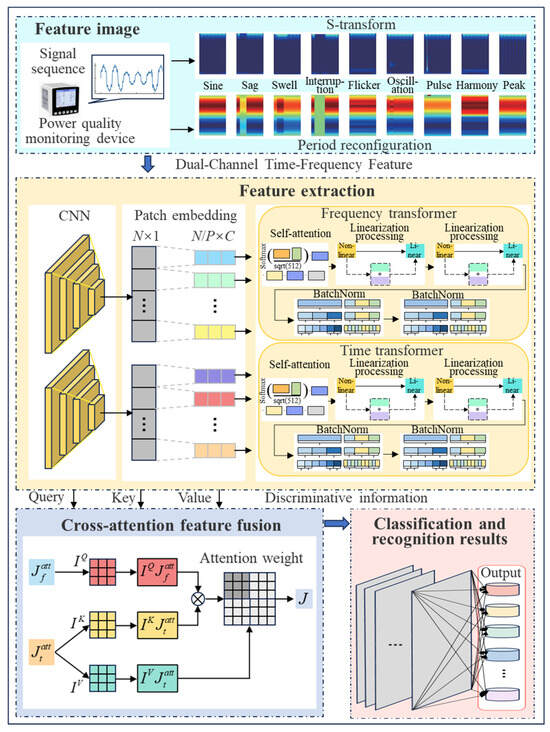
Figure 2. PQD identification method based on the dual-channel time–frequency feature fusion network.

3.1. Dual-Channel Time–Frequency Feature Composition

3.1.1. S-Transform

As a time–frequency analysis approach, the S-transform merges features of the short-time Fourier and wavelet transforms to generate a time–frequency representation of signals. Its core principle is to localize the signal in the time–frequency domain, analyzing it at varying times and frequencies by adjusting the window and modulation functions. This enables the S-transform to more effectively capture the nonlinear and unsteady characteristics of power quality interference signals, making it advantageous for processing nonlinear and transient signals. After removing burrs from the distribution terminal sampling sequence $\widehat{z}\left(m\right)$, the S transformation is performed, which can be expressed as follows:

$$S\left(\mu ,f\right)={\displaystyle {\int }_{-\infty }^{+\infty }\widehat{z}\left(m\right)g\left(m-\mu ,f\right)e^{-j2\pi ft}dm}$$

(12)

$$g\left(m-\mu ,f\right)={\displaystyle \frac{\left|f\right|}{\sqrt{2\pi }}}{e}^{{\displaystyle \frac{-{\left(m-\mu \right)}^2}{2{\sigma }^2}}}$$

(13)

where $g\left(m-\mu ,f\right)$ represents the Gaussian window function; $\sigma =1/fk$ is the window width factor; and $f$ is the frequency. $\mu$, as the translation factor, controls the position of the Gaussian window on the time axis. $\mu =kT$, where $T$ is the signal sampling period, and k is a constant.

3.1.2. Signal Period Reconfiguration

The complexity of PQD signal lies in its inherent multi-periodicity feature, which involves multiple periodic modes of different frequencies interweaving and influencing each other at the same time, resulting in highly complex temporal variations in the signal. In the traditional one-dimensional time series analysis method, due to its single dimension, it is easy to ignore or confuse the temporal variation in these different periods, which may seriously affect the validity and accuracy of the analysis’s results. Thus, based on the maximum frequency component of the power spectrum density of the PQD signal, the signal is converted into a two-dimensional matrix, which allows for the extraction of its multiple periodic patterns.

For the distribution terminal sampling sequence $\widehat{z}\left(m\right)$ after removing burrs, the discrete form is $\widehat{z}\left[n\right]$ and the length is $N$. It is divided into $R$ overlapping windows. The length of each window is $D$, and the overlapping length is $L$. The $r$-th window can be expressed as follows:

$${\widehat{z}}_r\left[n\right]={\widehat{z}}_r\left[n+r\left(D-L\right)\right],0\le n\le D,0\le r\le R$$

(14)

The signals within each window are then weighted. Let the window function be $u\left[n\right]$ and the weighted signal be expressed as follows:

$$q_r\left[n\right]={\widehat{z}}_r\left[n\right]u\left[n\right],0\le n\le D,0\le r\le R$$

(15)

Then, the weighted signal is transformed by Fourier transform. Define the Fourier transform as $F\left\{·\right\}$, which can be expressed as follows:

$$Q_r\left[m\right]=F\left\{q_r\left[n\right]\right\},0\le m\le M,0\le r\le R$$

(16)

Finally, the power spectral density $P\left[m\right]$ is calculated by using the average value of each segment, which can be expressed as follows:

$$P\left[m\right]={\displaystyle \frac{1}{R}}{\displaystyle \sum _{r=1}^{R-1}{Q}_r}\left[m\right],0\le m\le M$$

(17)

In power quality analysis, the significant frequency component of the power spectral density is crucial for understanding and processing disturbance signals. This component reveals the frequency with the most power, indicating the inherent periodic nature of the disturbance signal. By using this frequency, the new characteristic period of the signal is determined. After calculating the new period, the signal’s reconstruction period length is adjusted to be an integral multiple of the new period. This step preserves the signal’s periodic properties, preventing the introduction of non-original frequencies and maintaining the signal’s original periodic integrity. This method ensures that the reconstructed signal retains both the time and periodic characteristics of the original, making it easier to capture periodic disturbances such as harmonics and flickers. The frequency component with the most power is expressed as follows:

$$f_{\max }=\arg \max P\left[m\right]$$

(18)

$$length=T\left[{\displaystyle \frac{N}{T}}\right]$$

(19)

where $f_{\max }$ is the largest frequency component of the power spectral density $P\left[m\right]$, $T={\displaystyle \frac{1}{f_{\max }}}$ is the number of cycles, and $length$ is the length of the reconstructed signal.

When the computed new sequence ${\widehat{z}}_{\mathrm{p}\mathrm{a}\mathrm{d}}\left[n\right]$ exceeds the original one in length, the original sequence is filled and expressed as follows:

$${\widehat{z}}_{\mathrm{p}\mathrm{a}\mathrm{d}}\left[n\right]=\left\{\begin{array}{ll}\widehat{z}\left[n\right]\hfill & n<N\hfill \\ 0\hfill & N\le n<length\hfill \end{array}\right.$$

(20)

The completed sequence acquired by the distribution terminal is reshaped into a two-dimensional matrix X2D, enhancing the feature expression of PQD signals. In this matrix, each column and each row reflect the dynamic changes within a period and the periodic characteristics of signals over a week.

3.2. PQD Identification Based on the Twins Transformer

To effectively leverage frequency domain features for fault data and establish long-range dependencies with the Transformer, this paper introduces a more efficient Twins Transformer model. The Twins Transformer improves learning capability, accuracy, and generalization, boosting performance while reducing time complexity. The model includes a CNN-based convolutional feature extractor, a time–frequency domain Transformer encoder, a cross-attention feature fusion module, and an adaptive fault feature classifier shown in Figure 2. The CNN module employs a visual geometry group (VGG) architecture to extract both global temporal features and local spectral characteristics. The Transformer encoder subsequently captures multi-resolution representations across sensing domains, preserving long-range dependencies while identifying discriminative features. These refined features undergo cross-attention processing to strengthen inter-feature dependencies, enhancing diagnostic stability. For classification, an adaptive fault feature classifier mitigates computing overhead through parameter redundancy reduction, implementing global average pooling (GAP) followed by fully connected layers with nonlinear activations for multi-fault recognition.

3.2.1. CNN Feature Extraction Module

PQD datasets typically comprise time-domain signals containing both disturbance information and environmental noise. In PQD identification, signal features are divided into global and local categories. Global features represent the signal’s overall statistical or time-domain characteristics, while local features capture detailed time-domain information from specific segments, reflecting fine-grained disturbance traits.

Take $S\left(\tau ,f\right)$ and ${\widehat{z}}_{\mathrm{p}\mathrm{a}\mathrm{d}}\left[n\right]$ as inputs. By employing a CNN feature extraction module together with a Transformer for time feature extraction, the cross-attention mechanism effectively fuses features from both the time and frequency domains to form a comprehensive feature set for PQD classification. Due to its strong global feature capturing ability, VGG networks are widely used in object detection, image classification, and semantic segmentation tasks. In this work, the VGG network serves as the backbone to extract global features from PQD data and to map the input time-domain signals. The VGG architecture includes six convolutional layers, three pooling layers, and three batch normalization layers. Fully connected layers have been discarded, and the output from the third batch normalization layer serves as the final global feature.

3.2.2. Cross-Attention Feature Fusion Module

The PQD signal includes both disturbance and environmental noise. To emphasize the time-domain characteristics of disturbances and minimize noise interference, the Twins Transformer utilizes a self-focusing mechanism. This mechanism identifies features related to PQD while suppressing irrelevant environmental features, which can be expressed as follows:

$$J_t^{\mathrm{a}\mathrm{t}\mathrm{t}}=\mathrm{s}\mathrm{o}\mathrm{f}\mathrm{t}\max \left({\displaystyle \frac{J_{t_W}{J}_{t_C}}{\sqrt{b_t}}}\right)J_{t_V}$$

(21)

$$J_f^{\mathrm{a}\mathrm{t}\mathrm{t}}=\mathrm{s}\mathrm{o}\mathrm{f}\mathrm{t}\max \left({\displaystyle \frac{J_{f_W}{J}_{f_C}}{\sqrt{b_f}}}\right)J_{f_V}$$

(22)

where $J_t^{\mathrm{a}\mathrm{t}\mathrm{t}}$ and $J_f^{\mathrm{a}\mathrm{t}\mathrm{t}}$ represent the attention features of time-domain channel and frequency-domain channel, respectively. $J_{t_W}$, $J_{t_C}$, and $J_{t_V}$ all come from the time-domain channel feature $J_t$; $J_{f_W}$, $J_{f_C}$, and $J_{f_V}$ are derived from frequency domain channel features $J_f$; and $b_t$ and $b_f$ represent the dimensions of channel characteristics in the time domain and frequency domain. $\mathrm{s}\mathrm{o}\mathrm{f}\mathrm{t}\max \left(\right)$ is the activation function. The PQD signal exhibits diverse traits, such as vibration amplitude in the time domain and local damage timing in the frequency domain. To better capture detailed information from both domains, the cross-attention mechanism effectively merges time-domain features with local frequency-domain details. Through multiple layers of cross-attention, the model simultaneously focuses on different features and their complex interactions, significantly enhancing its ability to generalize.

The cross-attention fusion process of time-domain and frequence-domain feature modules is shown in Figure 2. By using the query matrix $I^H{J}_f^{\mathrm{a}\mathrm{t}\mathrm{t}}$ from $J_f^{\mathrm{a}\mathrm{t}\mathrm{t}}$ to calculate the cross concern of the feature matrix $J_t^{\mathrm{a}\mathrm{t}\mathrm{t}}$ to $J_f^{\mathrm{a}\mathrm{t}\mathrm{t}}$, the information exchange between the two feature matrices is strengthened, improving the integration of their features. Using self-attention for global time-domain features and local frequency-domain features, cross-attention is applied to enhance feature correlation and improve PQD identification. With the cross-attention and self-attention modules, correlations between points in the sequence are captured, offering discriminative information for PQD identification, as the correlation varies across different points and time series, which can be expressed as follows:

$$\begin{array}{cc}\hfill dis& =\mathrm{C}\mathrm{r}\mathrm{o}\mathrm{s}\mathrm{s}\_\mathrm{A}\mathrm{t}\mathrm{t}\mathrm{e}\mathrm{n}\mathrm{t}\mathrm{i}\mathrm{o}\mathrm{n}\left(J_t^{\mathrm{a}\mathrm{t}\mathrm{t}},J_f^{\mathrm{a}\mathrm{t}\mathrm{t}}\right)\hfill \\ & =\mathrm{s}\mathrm{o}\mathrm{f}\mathrm{t}\max \left({\displaystyle \frac{W_t{C}_t}{\sqrt{b_w}}}\right)V_t\hfill \\ & =\mathrm{s}\mathrm{o}\mathrm{f}\mathrm{t}\max \left({\displaystyle \frac{\left(I^C{J}_f^{\mathrm{a}\mathrm{t}\mathrm{t}}\right){\left(I^W{J}_t^{\mathrm{a}\mathrm{t}\mathrm{t}}\right)}^T}{\sqrt{b_w}}}\right)\left(I^V{J}_f^{\mathrm{a}\mathrm{t}\mathrm{t}}\right)\hfill \end{array}$$

(23)

where $I^C$, $I^W$, and $I^V$ represent learnable parameters; $b_w$ is the dimensional size of the query $Q$ vector. The multi-head attention score is calculated many times, and the different attention scores obtained by the multi-head attention mechanism are superimposed to obtain the superposed feature representation $E_T$ and its linear transformation $E_{ft}$, which can be expressed as follows:

$$E_T=Cat\left(\mathrm{C}\mathrm{r}\mathrm{o}\mathrm{s}\mathrm{s}\_\mathrm{A}\mathrm{t}\mathrm{t}\mathrm{e}\mathrm{n}\mathrm{t}\mathrm{i}\mathrm{o}\mathrm{n}\left(J_t^{\mathrm{a}\mathrm{t}\mathrm{t}},J_f^{\mathrm{a}\mathrm{t}\mathrm{t}}\right)\right)$$

(24)

$$E_{ft}=\mathrm{L}\mathrm{i}\mathrm{n}\mathrm{e}\mathrm{a}\mathrm{r}\left(E_T\right)$$

(25)

After adding and combining $E_{ft}$ and $J_t^{\mathrm{a}\mathrm{t}\mathrm{t}}$ based on the cross-attention mechanism, the resulting feature is represented as $E$. The attention mechanism is then used to compute the attention score. By extracting and fusing features with self-attention and cross-attention, the final PQD identification result is passed to the adaptive pooling layer for output, which can be expressed as follows:

$$E=E_{ft}+J_t^{\mathrm{a}\mathrm{t}\mathrm{t}}$$

(26)

$$\kappa =\mathrm{s}\mathrm{o}\mathrm{f}\mathrm{t}\max \left(O^T\tanh \left(O_{\mathrm{a}\mathrm{t}\mathrm{t}}F+b_{\mathrm{a}\mathrm{t}\mathrm{t}}\right)\right)$$

(27)

$$Y=E{\kappa }^T$$

(28)

where $O_{\mathrm{a}\mathrm{t}\mathrm{t}}$ is the weight matrix of the attention layer, $b_{\mathrm{a}\mathrm{t}\mathrm{t}}$ is the deviation vector, $O^T$ is the initialized random parameter matrix, and $\kappa$ is the weight assigned by the input.

The overall workflow of the power quality data augmentation and processing method for distribution terminals considering high-frequency sampling is shown in Figure 3.

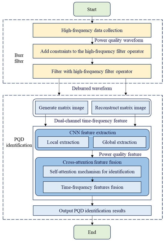
Figure 3. Power quality data augmentation and processing method for distribution terminals considering high-frequency sampling.

4. Experimental Results and Analysis

According to the IEEE Std 1159-2019 standard [23], a dataset was constructed considering the normal operating condition (C0) and eight types of single PQDs. The eight types of single PQDs are as follows: voltage spike (C1), voltage notch (C2), voltage flicker (C3), harmonics (C4), voltage sag (C5), voltage swell (C6), voltage interruption (C7), and transient oscillation (C8). The mathematical models for each disturbance are listed in Table 2. Based on the mathematical models provided in Table 2, the disturbances were generated with a sampling frequency of 12.8 kHz and a sampling length of 20 cycles, resulting in 640 sampling points per signal. Each type of disturbance included 300 samples. The dataset was divided into training (60%), validation (20%), and test (20%) sets according to standard proportions to ensure effective model learning and performance evaluation across different data subsets. The hardware and software settings are as follows. The CPU is Intel Core (TM) i7-1360P 2.20 GHz. The GPU is NVIDIA GeForce GTX 4060 with 8 GB of video memory. The running memory is 16 GB. The software version used is MATLAB 2019. The operating system is WINDOWS11 (64-bit). In the simulation of burr removal, the current waveform is used as an example. Table 3 lists the specific parameters [24,25]. Table 4 lists the key hyperparameters of the CNN and Transformer components [16,26].

Table 2. Modeling of various types of disturbance signals.

Disturbance Type	Mathematical Model	Constraint Condition
$C0$	$y\left(t\right)=\sin \left(\omega t\right)$	$A=1(pu),\omega =2\pi 50 \mathrm{rad}/\mathrm{s}$
$C1$	$\begin{array}{cc}\hfill y\left(t\right)& =\sin \left(\omega t\right)+sign\left(\sin \left(\omega t\right)\right)\hfill \\ & \times {\displaystyle \sum _{i=1}^{n}k\left[u\left(t-\left(t_1-0.02n\right)\right)-u\left(t-\left(t_2-0.02n\right)\right)\right]}\hfill \end{array}$	$\begin{array}{l}0\le t_1,t_2\le 0.5 \mathrm{T},0.1\le K\le 0.4\\ 0.01 \mathrm{T}\le t_2-t_1\le 0.05 \mathrm{T}\end{array}$
$C2$	$\begin{array}{cc}y\left(t\right)& =\sin \left(\omega t\right)-sign\left(\sin \left(\omega t\right)\right)\hfill \\ & \times {\displaystyle \sum _{i=1}^{n}k\left[u\left(t-\left(t_1-0.02n\right)\right)-u\left(t-\left(t_2-0.02n\right)\right)\right]}\hfill \end{array}$	$\begin{array}{l}0\le t_1,t_2\le 0.5 \mathrm{T},0.1\le K\le 0.4\\ 0.01 \mathrm{T}\le t_2-t_1\le 0.05 \mathrm{T}\end{array}$
$C3$	$y\left(t\right)=\left[1+{\alpha }_f\sin \left(\beta \omega t\right)\right]\sin \left(\omega t\right)$	$0.1\le {\alpha }_f\le 0.2,5\le \beta \le 20$
$C4$	$y\left(t\right)={\displaystyle \sum _{n″=1}^7{\alpha }_{n″}}\sin \left(n’’\omega t-v_{n″}\right)$	$n″=\left\{1,3,5,7\right\},0.05\le {\alpha }_{n″}\le 0.15$
$C5$	$y\left(t\right)=\left[1-\alpha \left(u\left(t-t_1\right)-u\left(t-t_2\right)\right)\right]\sin \left(\omega t\right)$	$0.1\le \alpha \le 0.9,T\le \left(t_2-t_1\right)\le 9 \mathrm{T}$
$C6$	$y\left(t\right)=\left[1+\alpha \left(u\left(t-t_1\right)-u\left(t-t_2\right)\right)\right]\sin \left(\omega t\right)$	$0.1\le \alpha \le 0.8,T\le \left(t_2-t_1\right)\le 9 \mathrm{T}$
$C7$	$y\left(t\right)=\left[1-\alpha \left(u\left(t-t_1\right)-u\left(t-t_2\right)\right)\right]\sin \left(\omega t\right)$	$0.9\le \alpha \le 1,T\le \left(t_2-t_1\right)\le 9 \mathrm{T}$
$C8$	$\begin{array}{cc}y\left(t\right)& =\sin \left(\omega t\right)\hfill \\ & +{\alpha }^{-\left(t-t_1\right)/\tau }\sin \left({\omega }_n\left(t-t_{1\prime }\right)\right)u\left(t-t_{2\prime }\right)-u\left(t-t_{1\prime }\right)\hfill \end{array}$	$8\le \tau \le \mathrm{40,300}\le f_n\le 900$

Table 3. Simulation parameters.

Parameter	Value	Parameter	Value
$T$	0.078125 ms	$N$	80
$D$	10	$R$	5
$L$	5	$b_t$	64
$length$	100	$b_f$	256

Table 4. Key hyperparameters of the CNN and Transformer components.

Key Hyperparameter	CNN	Transformer
Number of heads	\	8
Attention layer	\	6
Dropout	0.1	0.1
Learning rate	0.01	0.001
Number of training epochs	30	30
Batch size	128	128

Four baseline algorithms are used for comparison. The first two baselines represent traditional, widely used approaches. Baseline 1 [13] is a PQD identification method that uses a Kalman filter for automatic burr detection and removal. For this method, the filter gain was set to 0.05, the state noise covariance Q was diag (1 × 10⁻⁴), the observation noise covariance R was 0.01, and the iteration termination threshold was 1 × 10⁻⁶. Baseline 2 [14] combines time–frequency domain multi-features with a decision tree for disturbance identification. The decision tree was configured with a maximum depth of 12, a minimum of eight samples for a split, a feature sampling ratio of 0.8, and a pruning coefficient of 0.01. Its time–frequency features were extracted using a 200 ms window with 50% overlap. While these methods are valued for their low complexity and ease of deployment, they have notable limitations. Baseline 1’s reliance on single-domain signal processing compromises its robustness in complex noise environments. Baseline 2 does not address the crucial pre-processing step of burr removal, which impacts the quality of its input data. We also compare our work against two state-of-the-art deep learning models: STFT-CNN [20] (Baseline 3) and CNN-LSTM [21] (Baseline 4). The key hyperparameters for the CNN and Transformer components of these models, such as the number of heads and learning rate, are detailed in Table 4. Although these models leverage robust 2D data processing capabilities, they primarily operate on single-mode sequence features, neglecting the comprehensive integration of time–frequency dual characteristics that our method introduces.

To ensure a fair and rigorous comparison, all methods were evaluated under a unified training and testing framework. For the deep learning models, we employed the Adam optimizer and a uniform training schedule of 100 epochs, with an early stopping mechanism set with a patience of 10 epochs to prevent overfitting. This standardized procedure ensures that any observed performance differences are attributable to the architectural merits of the models rather than to variations in the training process. Moreover, both Baselines maintain identical input/output configurations and simulation parameter settings to the proposed algorithm.

Figure 4 shows the comparison of disturbance removal effects in the power quality data of different algorithms. The pre-filter power quality signal (C0) is affected by harmonics (C4), sag (C5), and transient oscillation (C8). Compared with Baseline 1 and 2, the proposed algorithm reduces the mean absolute error (MAE) by 62.73% and 75.26%, respectively. The reason for this is that the proposed algorithm uses high-frequency filtering operators for filtering. Based on a dual-channel time–frequency feature fusion network for deep feature analysis, it can eliminate disturbance while avoiding the signal distortion caused by filtering normal signals. As a result, it is able to improve the power quality data. However, Baseline 1 and 2 overlook the distinct disturbance characteristics in the signals and lack deep dual-domain feature fusion analysis, leading to poor high-frequency fault identification accuracy and degraded disturbance removal performance.

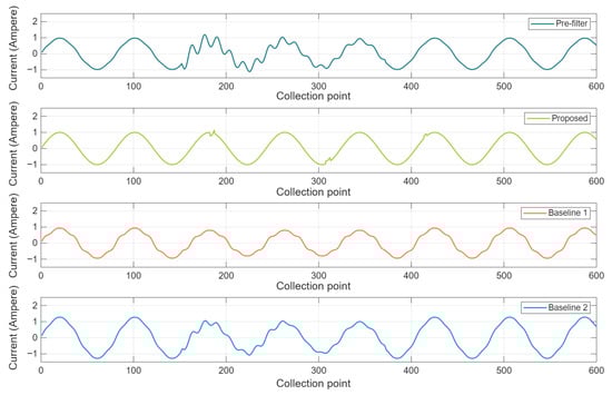
Figure 4. Comparison of disturbance removal effect in PQD of different algorithms.

Let $Z_1$ be the sampling value of the extreme point in the data after the current filtering point $m$. The extreme point does not align with the morphological characteristics of the unrestricted conditional shock operator. $Z_2$ is the sampling value with the smaller absolute value among the two sampling points with different values from $Z_1$ before and after the extreme value point. Thus, different restriction conditions can be adopted and expressed as follows:

$${\lambda }_1=\left|Z_1-Z_2\right|\times 1.5$$

(29)

$${\lambda }_2=3{\lambda }_1$$

(30)

where ${\lambda }_1$ is restriction condition 1 and ${\lambda }_2$ is restriction condition 2.

Figure 5 shows the comparison of the disturbance removal effects in the PQD of the proposed algorithm under different conditions. Compared with condition 1, the disturbance removal effect of conditions 2 is better. The reason for this is that condition 2, adopted by the proposed algorithm, only processes the sampled signals that conform to the disturbance characteristics. At the same time, a high-frequency filtering operator is applied to further filter the signal, thus preserving the effective information. However, condition 1 does not take into account the differential characteristics of disturbance, leading to the loss of some effective information. This, in turn, distorts the waveform of power quality data and negatively impacts the disturbance removal effect.

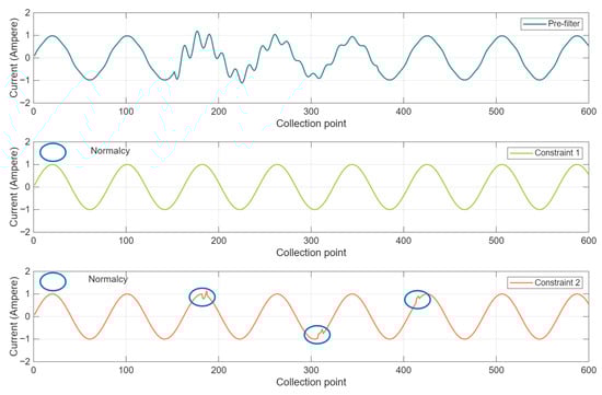
Figure 5. Comparison of disturbance removal effect in PQD of proposed algorithm under different conditions.

PQD identification is performed using the dataset, and the results are categorized into True Positives (TP), False Positives (FP), True Negatives (TN), and False Negatives (FN). TP denotes correctly predicted positive samples, FP represents negative samples incorrectly predicted as positive, TN refers to correctly predicted negative samples, and FN indicates positive samples incorrectly predicted as negative. Accuracy, precision, and recall are used to assess algorithm performance, which can be expressed as follows:

$$\begin{array}{l}Accuracy={\displaystyle \frac{TP+TN}{TP+TN+FP+FN}}\\ Precision={\displaystyle \frac{TP}{TP+FP}}\\ Recall={\displaystyle \frac{TP}{TP+FN}}\end{array}$$

(31)

Besides precision and recall, we introduce F1, which is a comprehensive evaluation metric for binary classification models to balance accuracy and recall. F1 is used to measure the accuracy and stability of the model in classification tasks, especially when the categories are imbalanced. F1 is expressed as follows:

$$F1={\displaystyle \frac{2\cdot Precision\cdot Recall}{Precision+Recall}}$$

(32)

Figure 6 shows the comparison of PQD identification accuracy over training iterations. Compared with Baseline 1, Baseline 2, Baseline 3, and Baseline 4, the identification accuracy of the proposed algorithm is improved by 21.33%, 16.98%, 11.37%, and 8.84%, respectively. The reason for this is that the proposed algorithm constructs the time–frequency domain dual-input features and processes them separately. It then couples the two features to enhance the PQD signal processing effect. However, Baseline 1 neglects the dual-channel time–frequency feature fusion network and fails to fully leverage disturbance signal characteristics, leading to reduced identification accuracy under the complex noise conditions in the distribution network. Baseline 2 lacks high-frequency filter operators, causing the distortion of high-frequency fault information and impacting the accuracy of disturbance identification. Baseline 3 and Baseline 4 process only single-mode sequence features, neglecting the interrelation between time and frequency domains as well as the complementary nature of multi-dimensional information. Consequently, under complex noise conditions in the distribution network, achieving precise signal characterization remains challenging, ultimately affecting detection performance.

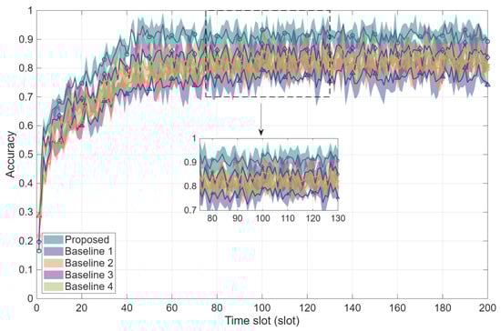
Figure 6. Comparison of PQD identification accuracy over training iterations.

Figure 7 illustrates the PQD identification accuracy of various algorithms against SNR. When SNR = 0 dB, the proposed algorithm improves its identification accuracy by 36.26%, 31.74%, 15.85%, and 16.22% compared to Baseline 1, 2, 3, and 4, respectively. Meanwhile, the proposed algorithm exhibits the smallest error bars among all Baselines. This improvement is due to the proposed algorithm’s use of the S-transform and signal period reconstruction to generate matrix image features, which are then input into the CNN to extract global time-domain and local frequency-domain features. Transformer encoders further extract highly coupled global features from the time–frequency sequences. The cross-attention mechanism captures long-term dependencies between sequences, enabling deep feature fusion. As a result, the identification accuracy and robustness of PQD are significantly enhanced in the complex noise environment of the distribution network.

Figure 7. PQD identification accuracy of different algorithms versus SNR.

Table 5 presents the PQD identification and classification results of the proposed algorithm at different noise levels. As the noise level decreases, the classification accuracy for 17 power quality events remains mostly at 100%, with the accuracy for disruption and vibration disturbances dropping to 97% and 98% at SNR = 30 dB. Additionally, the classification accuracy for some mixed disturbances (e.g., temporary drop + harmonic + vibration) falls to 95% at SNR = 30 dB. This demonstrates that the proposed algorithm maintains its robust performance and high accuracy even in high-noise-level environments, enabling effective PQD identification and classification. The algorithm works by preserving the key features of the original waveform while eliminating burrs through additional restrictions, and then extracting time–frequency domain features, allowing the classification layer to output accurate results even under high-noise-level conditions, significantly improving robustness and accuracy.

Table 5. PQD identification and classification results in different noise levels.

Disturbance Type	Accuracy/%
	30 dB	60 dB	90 dB	Noiseless
Sine	100	100	100	100
Temporary drop	99	99	98	100
Temporary rise	99	100	100	100
Disruption	97	99	100	100
Flicker	99	100	100	100
Vibration	98	100	100	100
Impulse	99	100	100	100
Harmonic	99	100	100	100
Notch	99	100	100	100
Peak	100	100	100	100
Temporary drop + Harmonic + Vibration	95	100	100	100
Temporary rise + Harmonic + Vibration	96	98	100	100
Temporary drop + Harmonic	97	100	100	100
Temporary rise + Harmonic	98	100	100	100
Temporary drop + Vibration	97	100	100	100
Temporary rise + Vibration	97	98	100	100
Harmonic + Vibration	97	100	100	100
Average	97.94	99.65	99.88	100

To further confirm the robustness and statistical significance of the proposed algorithm’s performance, we conducted five independent repeated experiments on the test set. For our proposed method, the mean accuracy was 97.9% with a 95% confidence interval of ±1.1%, and the mean F1-score was 97.7% with a 95% confidence interval of ±1.2%. A two-sided independent samples t-test was performed to compare the proposed algorithm against each of the four baseline methods, for both accuracy and the F1-score. Specifically, for accuracy, the t-statistics were 4.13 when compared to Baseline 1, 3.66 compared to Baseline 2, 2.55 compared to Baseline 3, and 2.87 compared to Baseline 4. For the F1-score, the t-statistics were 4.11 when compared to Baseline 1, 3.68 compared to Baseline 2, 2.54 compared to Baseline 3, and 2.89 compared to Baseline 4. The results consistently revealed statistically significant differences with $p<0.02$, favoring our proposed method. These findings strongly underscore the proposed algorithm’s superior and robust performance compared to existing methods, even under varying experimental conditions.

Figure 8 shows the relationship between PQD identification accuracy and the limiting parameter λ. As λ increases, the accuracy gradually declines because looser high-frequency filtering leaves more residual noise and weakens the extraction of critical fault-related components, which in turn affects feature representation and classification. To balance noise suppression and feature preservation in practical settings, λ should be adapted to the precision requirements of different operational scenarios. A practical workflow involves initializing λ based on the noise statistics of the signal first (e.g., λ_initial ≈ 1.2σ, where σ is the noise RMS), and then fine-tuning it according to the application. For transient-sensitive tasks such as detecting lightning-induced overvoltages or switching events, λ is typically tuned within a smaller range (0.10–0.25) to retain high-frequency fault signatures while suppressing noise. For routine periodic monitoring, where computational efficiency and signal smoothness are more important, a larger λ in the 0.25–0.45 range is preferable. This adaptive tuning strategy enables an effective trade-off between denoising performance and information integrity across diverse operational conditions.

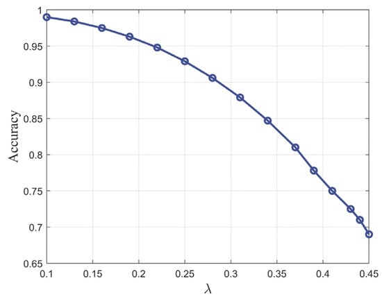
Figure 8. PQD identification accuracy versus λ.

Real-world disturbance data were used to validate the reliability of the proposed algorithm. The real-world PQD dataset used in this study consists of 1200 samples collected from the operational monitoring records of three regional 10 kV distribution substations, covering four mainstream types of distribution terminal units operating under different service conditions. The dataset includes eight typical PQD classes—voltage spike, notch, harmonics, sag, swell, interruption, flicker, and transient oscillation—along with a normal sinusoidal signal, ensuring sufficient diversity and representativeness for practical validation. In this paper, we ensure effective measurement of PQD baseline through data cleaning. We adopt the hybrid data cleaning framework using Markov Logic Networks (MLN) [27]. Firstly, infer a set of possible instantiation rules based on MLN, and then construct a two-layer MLN index structure to generate multiple data versions, facilitating the cleaning process. In the two-stage data cleaning step, we first propose the concept of reliability score to clean up errors in each data version separately and then use the new concept of the fusion score to eliminate conflicting values between different data versions.

Figure 9 presents the performance analysis of different algorithms under real-world disturbance data. The simulation results demonstrate that the proposed algorithm achieves the highest accuracy, precision, recall, and F1-score compared to the four baselines. This superiority stems from the algorithm’s innovative dual-channel time–frequency feature fusion network design and its optimization strategy for complex noise environments. By incorporating the dual-channel input and a cross-attention mechanism, the proposed method enhances both feature richness and noise robustness, enabling more accurate identification of various types of disturbances.

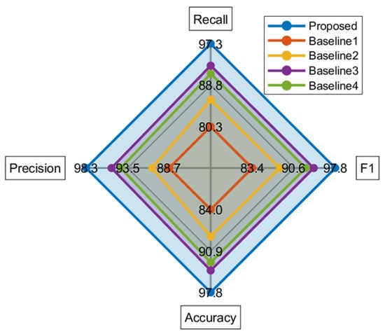
Figure 9. Performance analysis of different algorithms under real-world disturbance data.

To further validate the model’s practical applicability and statistical robustness, we performed 20 independent evaluations on the real-world disturbance dataset, and the results are visualized in Figure 10. The proposed algorithm consistently outperforms all baselines, achieving a superior median accuracy of 97.8%, which is a 3.9% improvement over the strongest baseline (Baseline 3) and a significant 16.4% gain over the weakest baseline (Baseline 1). Crucially, the proposed method also demonstrates the highest stability with the narrowest interquartile range, indicating reliable and consistent performance on unseen, real-world data. This consistency is attributed to the dual-channel network’s ability to extract rich, complementary features and the cross-attention mechanism’s effectiveness in enhancing noise robustness, allowing the model to generalize effectively from synthetic training to complex, practical scenarios.

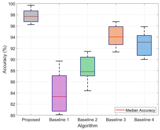
Figure 10. Statistical performance comparison on the real-world disturbance dataset.

The computing complexity of the proposed algorithm is composed of three parts, i.e., CNN feature extraction, a dual-path Transformer encoder, and cross-attention feature fusion. Specifically, the computing complexity of the CNN feature extraction part is $O\left(L·M·D\right)$, where $L$ is the number of power distribution terminals. $M$ is the length of the sampled sequence. $D$ is the feature dimension. The dual-path Transformer encode part has a computing complexity of $O\left(L·M^2·D\right)$. The cross-attention feature fusion part has a computing complexity of $O\left(L·M^2·D\right)$. Therefore, the total computing complexity is $O\left(L·M·D\right)+O\left(L·M^2·D\right)+O\left(L·M^2·D\right)\approx O\left(L·M^2·D\right)$. The computing complexities of Baseline 3 and Baseline 4 are also $O\left(L·M^2·D\right)$, which indicates the proposed algorithm has low complexity.

We have provided ablations to demonstrate the isolated contributions of the following factors: no burr filter, single channel, CNN only, Transformer only, and fusion without cross-attention, which are summarized in Table 6. The results underscore the importance of our key architectural innovations. The final analysis reveals that the burr removal, the dual-channel feature fusion strategy, and the cross-attention mechanism play crucial roles, contributing 5.39%, 1.38%, and 1.16% to the identification accuracy improvement, respectively.

Table 6. Performance comparison under the proposed algorithm with different components.

	Accuracy/%	Precision/%	F1-Score/%
No burr filter	92.83	93.41	91.59
Single channel	96.50	97.01	96.12
CNN only	93.92	94.14	92.50
Transformer only	95.17	95.83	94.57
Fusion without cross-attention	96.92	97.43	96.63
Proposed	97.83	98.32	97.82

5. Conclusions and Future Work

5.1. Conclusions

To address the distortion of high-frequency components and the lack of robustness in PQD identification in the face of complex distribution network noise, this study proposed a power quality data augmentation and processing framework tailored for high-frequency sampling at distribution terminals. A high-frequency filter operator with shape-preserving constraints was introduced to remove burrs while retaining critical transient features, significantly improving waveform fidelity. Building on the enhanced data quality, a dual-channel time–frequency feature fusion network was developed, where S-transform–based matrix images are reconstructed into dual inputs, extracted through CNN modules, and integrated via a cross-attention mechanism. Extensive simulations verify that the proposed method achieves notable improvements, including burr removal performance gains of 43.61% and 55.56% over two baselines, a 17.34% enhancement under unrestricted filtering, and PQD identification accuracy improvements of 21.33%, 16.98%, 11.37%, and 8.84% compared with four baselines.

5.2. Future Work

Despite the promising results, this study has several limitations that warrant discussion. First, there is a potential overfitting risk when applying the model, which has a substantial number of parameters, to real-world scenarios where high-quality labeled data may be limited. While techniques like data augmentation were used, their performance on unseen disturbance types or highly unique network conditions may vary. Second, the current model was developed and validated based on a fixed high-frequency sampling rate (12.8 kHz). Its real-time deployment under varying sampling rates (e.g., 8 kHz or 25.6 kHz), which are common in practical distribution terminals, presents a significant challenge. This would require adaptive input-shaping mechanisms or model retraining to maintain performance, impacting real-time feasibility and deployment complexity.

Future research will focus on advancing the practical deployment and scalability of the proposed method. We will explore hardware–software co-design for real-world implementation, including ARM-Cortex edge deployment with high-speed ADCs and detailed measurements of latency, memory usage, and inference speed to evaluate real-time feasibility. We also plan to further lightweight the model using hybrid quantization and knowledge distillation to maintain high accuracy under constrained computing resources. To strengthen cybersecurity resilience, we will integrate federated learning with GAN-based anomaly detection to build a more robust adversarial defense mechanism. In addition, we aim to automate the selection of the limiting parameter λ through data-driven optimization strategies, such as combining Bayesian optimization with cross-validation, ensuring adaptive tuning across diverse datasets. Furthermore, we will mitigate sensitivity to sampling jitter by developing a non-uniform sampling compensation algorithm based on phase-locked loop synchronization or quadratic interpolation, while exploring time series attention mechanisms to reduce the effect of timing deviations on feature extraction. Beyond these directions, we plan to explore the use of graph neural network-based models to further enhance generalization across complex grid scenarios, drawing on insights from recent GNN studies [28].

References

- Li, R.; Wong, P.; Wang, K.; Li, B.; Yuan, F. Power Quality Enhancement and Engineering Application with High Permeability Distributed Photovoltaic Access to Low-Voltage Distribution Networks in Australia. Prot. Control Mod. Power Syst. 2020, 5, 1–7. [Google Scholar] [CrossRef]
- Lv, H.; Wang, L.; Zhu, Y.; Du, W.; Liu, N.; Yang, D.; Cen, B. Harmonic Prediction of Power Grid Based on Improved SABO-BP Algorithm. Guangdong Electr. Power 2024, 37, 56–65. [Google Scholar]
- Bayrak, G.; Küçüker, A.; Yılmaz, A. Deep Learning-Based Multi-Model Ensemble Method for Classification of PQDs in A Hydrogen Energy-Based Microgrid Using Modified Weighted Majority Algorithm. Int. J. Hydrogen Energy 2023, 48, 6824–6836. [Google Scholar] [CrossRef]
- Li, D.; Channa, I.A.; Chen, X.; Dou, L.; Khokhar, S.; Ab Azar, N. A New Deep Learning Method for Classification of Power Quality Disturbances using DWT-MRA in Utility Smart Grid. Comput. Electr. Eng. 2024, 117, 109290–109291. [Google Scholar] [CrossRef]
- Eielsen, A.; Leth, J.; Fleming, A.; Wills, A.; Ninness, B. Large-Amplitude Dithering Mitigates Glitches in Digital-to-Analogue Converters. IEEE Trans. Signal Process 2020, 68, 1950–1963. [Google Scholar] [CrossRef]
- Tian, P.; Wu, G.; Chen, H.; Xie, T.; Tang, X.; Wang, R. Application of Temporal Convolutional Neural Network Combined with Autoencoder in Short-Term Bus Load Forecasting. In Proceedings of the 2020 Chinese Automation Congress (CAC), Shanghai, China, 6–8 November 2020; pp. 526–531. [Google Scholar]
- Xu, Q.; Miao, W.; Pong, P.W.T.; Liu, C. A Portable Power Quality Monitoring Approach in Microgrid with Electromagnetic Sensing and Computational Intelligence. IEEE Trans. Magn. 2021, 57, 4000506. [Google Scholar] [CrossRef]
- Ray, P.; Ray, P.; Dash, S. Power Quality Enhancement and Power Flow Analysis of a PV Integrated UPQC System in a Distribution Network. IEEE Trans. Ind. Appl. 2022, 58, 201–211. [Google Scholar] [CrossRef]
- Yılmaz, A.; Küçüker, A.; Bayrak, G.; Ertekin, D.; Shafie-Khah, M.; Guerrero, J.M. An Improved Automated PQD Classification Method for Distributed Generators with Hybrid SVM-based Approach using Un-Decimated Wavelet Transform. Int. J. Electr. Power Energy Syst. 2022, 136, 107763–107764. [Google Scholar] [CrossRef]
- Zhu, R.; Liu, S.; Peng, X.; Zhang, G.; Zeng, G.; Yin, J. Detection and Analysis of Voltage Sag Based on RSI-LMD. Guangdong Electr. Power 2022, 35, 60–69. [Google Scholar]
- Tang, Q.; Qiu, W.; Zhou, Y. Classification of Complex Power Quality Disturbances using Optimized S-Transform and Kernel SVM. IEEE Trans. Ind. Electron. 2020, 67, 9715–9723. [Google Scholar] [CrossRef]
- Rahul. Dual Tree Complex Wavelet Transform with Multiobjective Optimization Algorithm for Real-Time Power Quality Events Classification. Adv. Theor. Simul. 2020, 3, 2000141–2000142. [Google Scholar] [CrossRef]
- Abdelsalam, A.A.; Abdelaziz, A.Y.; Kamh, M.Z. A Generalized Approach for Power Quality Disturbances Identification Based on Kalman Filter. IEEE Access 2021, 99, 93614–93628. [Google Scholar] [CrossRef]
- Zhao, W.; Shang, L.; Sun, J. Power Quality Disturbance Classification based on Time-Frequency Domain Multi-Feature and Decision Tree. Prot. Control. Mod. Power Syst. 2019, 4, 27. [Google Scholar] [CrossRef]
- Duan, Z.; Peng, Z.; Song, J.; Lu, S. An Intelligent Complex Power Quality Disturbance Identification Method based on Two Dimension Encoding Conversion And Machine Vison. Electr. Power Syst. Res. 2024, 232, 110413–110414. [Google Scholar] [CrossRef]
- Cui, C.; Duan, Y.; Hu, H.; Wang, L.; Liu, Q. Detection and Classification of Multiple Power Quality Disturbances Using Stockwell Transform and Deep Learning. IEEE Trans. Instrum. Meas. 2022, 71, 2519912. [Google Scholar] [CrossRef]
- He, M.; Li, J.; Mingotti, A.; Tang, Q.; Peretto, L.; Teng, Z. Deep Fractional Multidimensional Spectrum Convolutional Neural Fusion Network for Identifying Complex Power Quality Disturbance. IEEE Trans. Instrum. Meas. 2024, 73, 9005412. [Google Scholar] [CrossRef]
- Bashir, T.; Wang, H.; Tahir, M.; Zhang, Y. Wind and Solar Power Forecasting Based on Hybrid CNN-ABiLSTM, CNN-Transformer-MLP Models. Renew. Energy 2025, 239, 122055–122056. [Google Scholar] [CrossRef]
- Yoon, D.; Yoon, J. Development of a Real-Time Fault Detection Method for Electric Power System via Transformer-Based Deep Learning Model. Int. J. Electr. Power Energy Syst. 2024, 159, 110069–110070. [Google Scholar] [CrossRef]
- Chen, Z.; Yi, Q.; Xu, H.; Guo, D. Deep STFT-CNN for Spectrum Sensing in Cognitive Radio. IEEE Commun. Lett. 2021, 25, 864–868. [Google Scholar] [CrossRef]
- Zhou, Q.; Tang, J. An Interpretable Parallel Spatial CNN-LSTM Architecture for Fault Diagnosis in Rotating Machinery. IEEE Internet Things J. 2024, 11, 31730–31744. [Google Scholar] [CrossRef]
- Thomas, J.B.; Chaudhari, S.G.; Shihabudheen, K.V.; Verma, N.K. CNN-Based Transformer Model for Fault Detection in Power System Networks. IEEE Trans. Instrum. Meas. 2023, 72, 2504210. [Google Scholar] [CrossRef]
- IEEE Std 1159-2019; IEEE Recommended Practice for Monitoring Electric Power Quality. IEEE: New York, NY, USA, 2019.
- Gao, Z.; Wang, Y.; Li, X.; Yao, J. Twins Transformer. Rolling Bearing Fault Diagnosis based on Cross-Attention Fusion of Time and Frequency Domain Features. Meas. Sci. Technol. 2024, 10, 96113–96114. [Google Scholar] [CrossRef]
- Qin, R.; Xu, Z.; Kuang, H.; Jiang, H.; Xi, X.; Ren, M. Detection Method of Power Quality Disturbances Based on Double Resolution S Transform and Improved Multi-scale ResNet. Guangdong Electr. Power 2024, 37, 68–77. [Google Scholar]
- Nguyen, P.T.-T.; Kuo, C.-H. A Novel Surface Electromyographic Gesture Recognition Using Discrete Cosine Transform-Based Attention Network. IEEE Signal Process Lett. 2024, 31, 266–270. [Google Scholar] [CrossRef]
- Ge, C.; Gao, Y.; Miao, X.; Yao, B.; Wang, H. A Hybrid Data Cleaning Framework Using Markov Logic Networks. IEEE Trans. Knowl. Data Eng. 2022, 34, 2048–2062. [Google Scholar] [CrossRef]
- Liang, Z.; Yin, X.; Chung, C.Y.; Rayeem, S.K.; Chen, X.; Yang, H. Managing Massive RES Integration in Hybrid Microgrids: A Data-Driven Quad-Level Approach With Adjustable Conservativeness. IEEE Trans. Ind. Inform. 2025, 21, 7698–7709. [Google Scholar] [CrossRef]
Disclaimer/Publisher’s Note: The statements, opinions and data contained in all publications are solely those of the individual author(s) and contributor(s) and not of MDPI and/or the editor(s). MDPI and/or the editor(s) disclaim responsibility for any injury to people or property resulting from any ideas, methods, instructions or products referred to in the content. |
© 2025 by the authors. Licensee MDPI, Basel, Switzerland. This article is an open access article distributed under the terms and conditions of the Creative Commons Attribution (CC BY) license (https://creativecommons.org/licenses/by/4.0/).