Optimal Power Flow-Assisted Unit Commitment with Multi-Level Load Variation Analysis in Renewable-Based Power Systems

Abstract

High penetration of distributed photovoltaic (PV) generation introduces operational challenges for thermal power plants, including increased cycling, higher losses, and reduced system flexibility. This study proposes an integrated optimization framework that combines Mixed Integer Nonlinear Programming (MINLP)-based Unit Commitment (UC) with a Particle Swarm Optimization (PSO)-assisted Optimal Power Flow (OPF) solved using the Newton–Raphson method. Applied to the IEEE 30-bus system for a 24-h horizon, the UC stage schedules 3717.8 MW of thermal generation at a cost of $8771.14. Load flow validation indicates a required supply of 3793.7 MW due to network losses, increasing the cost to $9031.64 and causing several constraint violations. The PSO-assisted OPF resolves all violations and produces an adjusted total generation of 3778.5 MW, reducing losses and lowering the overall operating cost to $8912.47 through optimal redispatch and voltage regulation. To further evaluate system robustness, multiple load scenarios—including reduced, nominal, and increased demand—are analyzed. Across all scenarios, the OPF stage is able to eliminate operational violations, decrease real power losses, and maintain voltage profiles within acceptable limits, demonstrating consistent performance under varying system stress levels. Overall, the integrated UC–OPF framework enhances economic efficiency, operational reliability, and resilience under renewable variability and shifting load conditions.

1. Introduction

The rapid transition toward sustainable energy systems has significantly accelerated the integration of renewable energy sources, particularly photovoltaic (PV) systems, into modern power networks [1,2,3]. This transformation is largely motivated by the global imperative to mitigate greenhouse gas emissions and reduce reliance on fossil-based generation, which is both finite and environmentally harmful [4,5]. PV technology utilizes the photovoltaic effect to convert solar irradiance into electrical energy [6]. Continuous improvements in conversion efficiency, along with decreasing capital costs, have further accelerated its adoption across residential, commercial, and industrial sectors [7,8].

Despite its advantages, the variability and intermittency of solar energy introduce substantial operational challenges to power system management [9,10]. Solar generation fluctuates throughout the day and ceases entirely at night or under adverse meteorological conditions. Such stochastic variations can disrupt the balance between generation and demand, affect voltage profiles, and necessitate frequent cycling of thermal units—thereby increasing start-up costs and decreasing overall system efficiency [9,11,12,13]. To mitigate these adverse impacts, various control and compensation strategies have been investigated, including PV curtailment [2] and the incorporation of Energy Storage Systems (ESSs) [14,15,16,17]. Among available ESS technologies, Pumped Hydro Storage (PHS) stands out due to its high round-trip efficiency, large energy capacity, and technical maturity. The advantage of PHS is that it is particularly suitable for large-scale renewable-integrated grids [18]. In this context, Distributed Generation (DG) units—such as PV systems, wind turbines, and small hydro plants—play a vital role in enhancing grid flexibility and local reliability. However, their distributed and intermittent nature also increases the complexity of system operation planning, especially when coordinating with centralized thermal generation and storage systems.

In system operation planning, the Unit Commitment (UC) problem plays a central role. UC determines the optimal on/off scheduling of generating units over a specified time horizon while adhering to numerous operational and technical constraints [19,20]. These constraints encompass generator limits, ramp rate restrictions, minimum up/down times, and increasingly, network-level constraints derived from power flow equations [21,22,23]. To ensure that bus voltages and line loadings remain within permissible limits, Optimal Power Flow (OPF) analysis is often incorporated into UC frameworks [24,25]. The OPF problem itself is typically addressed using numerical approaches such as the Gauss–Seidel or Newton–Raphson methods [8], which provide a detailed representation of network physics and power balance relationships [26,27].

However, the combined UC with OPF problem is inherently nonlinear, nonconvex, and NP-hard, particularly when renewable generation uncertainty and time-coupled operational limits are included [22,24,28]. Conventional mathematical optimization techniques, such as Mixed-Integer Nonlinear Programming (MINLP), are capable of producing accurate solutions but at the expense of significant computational burden [28,29]. In contrast, metaheuristic algorithms—such as PSO—are computationally efficient and well-suited for complex optimization problems, though they may converge prematurely and fail to reach the true global optimum [30,31,32,33]. To achieve a balance between computational efficiency and solution optimality, hybrid optimization frameworks that integrate deterministic and metaheuristic methods have emerged as promising alternatives.

A broad range of studies have been conducted to address the UC problem under various operational contexts. For example, Ref. [34] adopted a multi-objective compromise programming approach to minimize generation cost, emissions, and wind curtailment; however, power flow considerations were omitted. A hybrid priority-list and modified firefly algorithm was utilized in Ref. [35] for thermal unit scheduling, but renewable sources and network constraints were excluded. Similarly, Ref. [36] proposed a stochastic MILP formulation for combined heat and power (CHP) plants and virtual power plants, yet power flow analysis was not incorporated. Reinforcement learning-based methods, such as the PPO-D framework in [37], have demonstrated effectiveness in addressing wind power uncertainty on large-scale systems, though without considering PV integration or OPF. Meanwhile, Ref. [38] integrated electric vehicle charging and battery storage into a stochastic MILP UC model that included power flow constraints. More recently, Ref. [39] introduced a PSO–GWO hybrid approach for solar-integrated power systems, focusing on PV intermittency but without coupling UC scheduling.

From the reviewed literature, it is evident that a fully integrated framework that simultaneously considers renewable energy variability, Unit Commitment (UC) scheduling, and OPF-assisted dispatch has not been comprehensively explored. In contrast to previous studies, the incremental contribution of this work is threefold. First, we develop an integrated UC–OPF framework that simultaneously optimizes commitment schedules and real-time dispatch while explicitly incorporating both photovoltaic (PV) units and pumped hydro storage (PHS), a combination that has rarely been addressed jointly in the literature. Second, unlike approaches that treat UC and network-constrained dispatch in isolation, our method sequentially solves the UC problem using a MINLP formulation and subsequently refines the dispatch through a PSO-assisted Newton–Raphson OPF solver, ensuring that the final solution satisfies both economic scheduling and system-wide operational constraints under renewable uncertainty. Third, we validate the framework under multiple loading conditions and demonstrate measurable improvements in total operating cost, system losses, and voltage stability, thereby reinforcing its suitability for mixed renewable–hydro configurations.

To bridge the identified research gap, the present study aims to develop an optimization strategy that achieves economically optimal and operationally feasible dispatch while maintaining network reliability under fluctuating PV generation in renewable-integrated power systems. Furthermore, the robustness of the proposed framework is evaluated by analyzing its performance under varying demand levels, providing insights into how different loading conditions influence UC–OPF decisions and overall system behavior.

2. System Model

In this study, the input data consist of the characteristics of thermal generators and PV units, the 24-h load profile, and the specifications of the pumped hydro storage (PHS). The datasets used are primarily based on the IEEE 30-bus system described in [40], as originally introduced in the IEEE Power Systems Test Case Archive, while additional parameters related to the UC, PV generation profile, PHS specifications, and 24-h load data are adapted from [41], which conducted a similar hybrid generation scheduling study. All numerical data applied in Table 1, Table 2, Table 3, Table 4 and Table 5 have been derived or adapted from these two sources to ensure consistency and reproducibility of the test system configuration.

Table 1. Operational cost characteristics of generators.

Generator	Fuel Cost Function ($)
	a	b	c
Slack	0.02000	2.00000	0
Thermal 1	0.01750	1.75000	0
Thermal 2	0.06250	1.00000	0
Thermal 3	0.00834	3.25000	0
Thermal 4	0.02500	3.00000	0
Thermal 5	0.02500	3.00000	0

Table 2. Active and reactive power limit for generators.

Generator	Bus	Active Power Limit (MW)		Reactive Power Limit (Mvar)		Voltage Limit (pu)
		Max	Min	Max	Min	Max	Min
Slack	0	80	0.0	150	−20	1.05	0.95
Thermal 1	1	80	0.0	60	−20	1.1	0.95
Thermal 2	20	50	0.0	62.5	−15	1.1	0.95
Thermal 3	22	55	0.0	48.7	−15	1.1	0.95
Thermal 4	21	30	0.0	40	−10	1.1	0.95
Thermal 5	26	30	0.0	40	−10	1.1	0.95

Table 3. Operational Constraints Data of Thermal Generators.

Unit	Pmax (MW)	Pmin (MW)	Minimum Up Time	Minimum Down Time
1	162	25	3.00	3.00
2	55	10	1.00	1.00
3	55	10	2.00	2.00
4	55	10	2.00	2.00
5	85	25	2.00	1.00
6	130	20	2.00	2.00

Table 4. PHS Specification Data.

Parameter	PHS 1
PHS Maximum Power Output (MW)	60
PHS Maximum Capacity (MWh)	518
Efficiency (%)	85
Minimum Down Time (jam)	1
Minimum Up Time (jam)	1
Operational Cost ($)	5.5

Table 5. 24-h Load Data.

Hour	Load (MW)	PV Output (MW)	Hour	Load (MW)	PV Output (MW)
1	135.4	0.0	13	186.5	77.3
2	128.3	0.0	14	190.0	85.9
3	125.6	0.0	15	186.5	64.9
4	126.4	0.0	16	183.4	51.4
5	129.4	0.0	17	177.4	29.7
6	114.9	0.0	18	180.2	19.2
7	102.6	2.4	19	185.6	5.9
8	107.3	8.2	20	186.5	0.0
9	126.7	26.1	21	178.8	0.0
10	148.8	41.8	22	169.3	0.0
11	165.2	54.2	23	160.2	0.0
12	175.3	57.7	24	147.7	0.0

An illustration of the tested system configuration is presented in Figure 1. Based on Figure 1, it can be observed that the energy sources consist of thermal generators, PHS, and PV farms. These components are connected to the main power grid, with breakers placed between the interconnections. This study assumes that all of these elements operate under a single Unit Commitment framework. The test system consists of the IEEE 30-bus network with six thermal generating units and one PHS unit. The generator cost, operating limits, and UC constraints are summarized in Table 1, Table 2, Table 3 and Table 4, while the 24-h load and PV output data used for simulation are presented in Table 5.

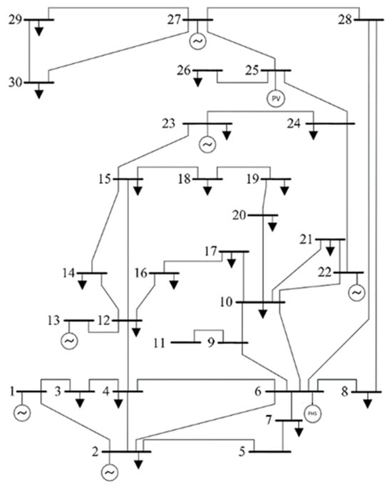
Figure 1. The testing system configuration used. The numbers denote the bus numbers of the IEEE 30-bus test system.

In the scheduling formulation, the minimum downtime of the pumped-storage hydro (PHS) unit is set to 1 h, as shown in Table 4. This assumption aligns with the hourly time-step adopted in this study and reflects the high operational flexibility of modern pumped-storage plants, where start-up times as short as a few minutes have been reported. Although the actual minimum downtime may vary depending on site-specific hydraulic and mechanical constraints, the one-hour setting is considered appropriate for the hourly scheduling horizon of this work.

To evaluate the robustness and adaptability of the proposed optimization framework, several load-scaling scenarios were applied. The total system load was proportionally adjusted to 50%, 75%, 125%, and 150% of the base case. This scaling process aims to examine whether the PSO–NR algorithm can maintain optimal performance and convergence under varying system stress levels. In addition, it allows analysis of how Pumped Hydro Storage (PHS) contributes to system stability and cost efficiency across light-load and heavy-load conditions. The scenarios also provide insight into generator commitment flexibility, transmission loading limits, and the capability of renewable integration under different demand levels.

3. Problem Mathematical Modeling

This section presents the mathematical formulation of the proposed optimization problem, which combines UC and OPF models into an integrated framework. The UC problem determines the optimal scheduling of thermal generators and Pumped Hydro Storage (PHS) units, while the OPF ensures that power flows in the network satisfy operational constraints.

3.1. Unit Commitment Formulation (MINLP)

• Objective Function of Unit Commitment

$$\mathit{min}F=\sum _{t=1}^{NT}\left\{\sum _{i=1}^{NG}\left(F{C}_i\left(P_{GTi}\left(t\right)\right)+SUC\left(t\right)+SDC\left(t\right)\right)+\sum _{i=1}^{NPHS}{CPHS}_i\left(t\right)\right\}$$

(1)

where F is objective function of economic dispatch, NT is operation period of the generator (hours), NG is numbers of generator, $F{C}_i\left(P_{gi}\left(t\right)\right)$ is generator fuel cost, SUC(t) is generator start-up cost, SDC(t) is generator shut-down cost, and CPHS is PHS operational cost

a.

Fuel Cost Function of Thermal Generators

$$F{C}_i\left(P_{GTi}\left(t\right)\right)={\left(\right(a}_i+b_i{P}_{GTi}\left(t\right)+c_i{P_{GTi}\left(t\right)}^2)$$

(2)

where a, b and c are generator fuel cost coefficients.

b.

Startup Cost Model of Thermal Generators

$$SUC(t)=\sum _{i=1}^{NTG}SUC(u_{i,t}-u_{i,(t-1)}) u_{i,t}$$

(3)

where u is the state of the generator. One is when the generator is on and zero is when the generator is off.

c.

Shutdown Cost Model of Thermal Generators

$$SDC(t)=\sum _{i=1}^{NTG}SDC(u_{i,\left(t-1\right)}-u_{i,t}) u_{i,(t-1)}$$

(4)

d.

Operational Cost Model of PHS

$${CPHS}_i\left(t\right)={PHS}_{output}{OPHS}_i$$

(5)

where OPHS_i is PHS operational cost coefficient

2.

Unit Commitment Constraint Model

There are several constraints that must be satisfied in the optimization of Unit Commitment. These constraints can be categorized into three groups: power balance constraints, thermal generator constraints, and PHS operation constraints. The power balance constraint requires that the total load must be equal to the total power generated in each period. Thermal generator constraints are defined based on the specifications of each thermal unit. Meanwhile, the PHS constraints are determined according to the technical specifications of the pumped hydro storage system used.

a.

Power Balance Constraint Model

$$P_{LD}(t)=\sum _{i=1}^{NTG}{P}_{GTi}(t)+\sum _{i=1}^{NPV}{P}_{PVi}\left(t\right)+\sum _{i=1}^{NPSH}{P}_{{PSH}_{op i}}\left(t\right)-\sum _{i=1}^{NPSH}{P}_{{PSH}_{in i}}\left(t\right)$$

(6)

where $P_{GTi}$ is thermal generator production power, $P_{PVi}$ is PV output power, $P_{{PHS}_{op i}}$ PHS output power, $P_{{PHS}_{in i}}$ is PHS input power

b.

Thermal Generator Power Output Constraint

$$P_{{GT}_i}^{min}\le P_{{GT}_{i }}\le P_{{GT}_i}^{max}$$

(7)

where $P_{{GT}_i}^{min}$ is generator minimum power and $P_{{GT}_i}^{max}$ is generator maximum power

c.

Thermal Generator Minimum Up-Time Constraint

$$MU{T}_i{ u}_{i,t}\left(u_{i,t}-u_{i,\left(t-1\right)}\right)=\sum _{t=1}^{t=MU{T}_i}{u}_{i,t}$$

(8)

where $MU{T}_i$ is generator minimum up-time

d.

Thermal Generator Minimum Down-Time Constraint

$$MD{T}_i{ u}_{i,\left(t-1\right)}\left(u_{i,t-1}-u_{i,t}\right)=\sum _{t=1}^{t=MD{T}_i}{u}_{i,t}$$

(9)

where $MD{T}_i$ is generator minimum down-time

e.

PHS Capacity Constraint Model

$$C_{PHS}{\left(t\right)}_i=C_{PHS}{(t-1)}_i+P_{{PHS}_{input i}}\left(t\right)-P_{{PHS}_{output i}}\left(t\right)$$

(10)

3.2. Power Flow Constraint

The system power flow is governed by the standard AC power flow equations, ensuring that all bus voltages and power injections are balanced according to network topology and admittance. This formulation is used later for optimization using the PSO–NR approach.

a.

Power Balance Constraints

$$P_k=V_k\sum _n^N{V}_n[G_{kn}\cos \left({\mathsf{\theta }}_k-{\mathsf{\theta }}_n\right)+B_{kn}\sin \left({\mathsf{\theta }}_k-{\mathsf{\theta }}_n\right)]$$

(11)

$$Q_k=V_k\sum _n^N{V}_n[G_{kn}\sin \left({\mathsf{\theta }}_k-{\mathsf{\theta }}_n\right)-B_{kn}\cos \left({\mathsf{\theta }}_k-{\mathsf{\theta }}_n\right)]$$

(12)

where $V_k$ and $V_n$ represent the voltage magnitudes at buses k and n, respectively, expressed in per unit (pu) or volts. The angles ${\mathsf{\theta }}_k$ and ${\mathsf{\theta }}_n$ denote the voltage phase angles at the corresponding buses, measured in radians. Meanwhile, $G_{kn}$ and $B_{kn}$ are the real and imaginary components of the mutual admittance between buses k and n, which constitute the elements of the bus admittance matrix Ybus.

b.

Bus Voltage Limits

$$V_k^{min}\le V_k\le V_k^{max}$$

(13)

where ${\mathrm{V}}_{\mathrm{k}}^{\mathrm{m}\mathrm{i}\mathrm{n}}$ is minimum voltage at bus k and ${\mathrm{V}}_{\mathrm{k}}^{\mathrm{m}\mathrm{a}\mathrm{x}}$ is maximum voltage at bus k.

c.

Generator Reactive Power Limits

$$Q_{Gi}^{min}\le {Q_{Gi}\le Q}_{Gi}^{max}$$

(14)

where ${\mathrm{Q}}_{\mathrm{G}\mathrm{i}}^{\mathrm{m}\mathrm{i}\mathrm{n}}$ is generator minimum reactive power and ${\mathrm{Q}}_{\mathrm{G}\mathrm{i}}^{\mathrm{m}\mathrm{a}\mathrm{x}}$ is generator maximum reactive power.

4. Integrated MINLP–PSO Framework for Unit Commitment and Optimal Power Flow

The proposed optimization framework integrates Mixed-Integer Nonlinear Programming (MINLP) for UC with PSO for OPF. The MINLP formulation determines the optimal on/off status and generation levels of thermal and PHS units, while the PSO algorithm refines the power dispatch and voltage profiles by solving the OPF problem under network constraints. This hybrid strategy ensures both economic efficiency and operational feasibility in power system operation.

The integration between UC and OPF is carried out in a two-stage optimization process. In the first stage, the UC problem formulated as an MINLP determines which generating units should be committed at each scheduling period based on fuel cost, ramp limits, and minimum up/down-time constraints.

In the second stage, the PSO-based OPF optimization computes the optimal active and reactive power outputs and voltage magnitudes for the committed units while satisfying AC power flow constraints.

4.1. MINLP Optimization with SCIP

The first stage of the proposed framework involves solving the UC problem formulated as a Mixed-Integer Nonlinear Programming (MINLP) model. In this study, the SCIP (Zuse Institute Berlin (ZIB), Berlin, Germany) optimization solver is employed due to its robustness in handling both integer and nonlinear constraints simultaneously, which are inherently present in UC problems [42,43,44]. SCIP integrates branch-and-bound strategies with nonlinear relaxation techniques, allowing efficient convergence even for problems involving both discrete scheduling decisions and continuous power balance equations.

In this research, the UC formulation is expanded into a large-scale MINLP problem consisting of six generating units, including both thermal and Pumped Hydro Storage (PHS) plants, evaluated over a 24-h scheduling horizon. The PV is included to in this system. This results in hundreds of binary variables and nonlinear equality and inequality constraints that represent unit operating limits, minimum up/down times, ramping capabilities, and power balance constraints. Rather than manually tuning each combination, the SCIP solver automatically explores feasible configurations using mixed-integer strategies until an optimal or near-optimal schedule is achieved [43].

Furthermore, SCIP’s internal presolving routines and constraint propagation significantly reduce computational burden by eliminating infeasible or redundant variable bounds early in the optimization process [44]. This makes SCIP particularly suitable for large-scale UC problems integrated with renewable and storage systems, where nonlinearity arises from efficiency curves, variable costs, and energy storage dynamics. The resulting output from this stage—i.e., the optimal ON/OFF schedule and initial generation levels for each unit—serves as the initial input for the subsequent PSO-based OPF optimization stage.

4.2. PSO-Assisted Optimal Power Flow Under UC Constraints

In the second stage of the proposed framework, the OPF problem is solved using the PSO algorithm, which operates under the commitment schedule determined by the MINLP-based UC model. While the first stage identifies which generating units are online and provides their preliminary dispatch levels, the second stage refines the generation dispatch by minimizing the total operating cost and network losses while satisfying the nonlinear power flow constraints.

The PSO algorithm is selected due to its robust global search capability and ease of adaptation for complex, nonconvex optimization problems such as OPF [45]. In this work, PSO is employed to optimize, reactive power, and voltage magnitude of generator buses while maintaining the power balance equations and essential system operating limits, including generator capacity and bus voltage constraints.

The fitness function of each particle is evaluated using the Newton–Raphson (NR) load flow method, which accurately computes power mismatches, network losses, and voltage profiles for each candidate solution [46]. This coupling of PSO with NR ensures that the optimization process not only minimizes total generation cost but also maintains feasible and stable network operation under all considered load and generation conditions.

Each particle in the PSO population represents a potential solution consisting of the active power, reactive power, and voltage of the generator buses. The dimension of the particle is therefore determined by the number of generator variables included in the optimization [47]. The velocity and position of each particle are iteratively updated according to the standard PSO equations:

$$v_i^{(k+1)}=\mathsf{\omega }{v}_i^{\left(k\right)}+c_1{r}_1\left(p_i^{best}-x_i^{\left(k\right)}\right)+c_2{r}_2\left(g^{best}-x_i^{\left(k\right)}\right)$$

$$x_i^{(k+1)}=x_i^{\left(k\right)}+v_i^{(k+1)}$$

where v_i and x_i denote the velocity and position of the i-th particle, respectively; $p_i^{best}$ and $g^{best}$ are the local and global best positions; r₁, r₂ ∈ [0, 1] are random coefficients; c₁ and c₂ are acceleration constants; and ω is the inertia weight controlling exploration and exploitation balance.

The fitness function of each particle is designed to reflect the economic and operational performance of the system. It is defined as:

$$F_{penalty}= F{C}_i\left(P_{GTi}\left(t\right)\right)+{\mathsf{\lambda }}_p{f}_p+{\mathsf{\lambda }}_q{f}_q+{\mathsf{\lambda }}_v{f}_v+{\mathsf{\lambda }}_{ramp}{f}_{ramp}+{\mathsf{\lambda }}_{nr}{f}_{nr}$$

where $f_p$, $f_q$, $f_v$, $f_{ramp}$, and $f_{nr}$ denote the active and reactive power mismatch penalties derived from the Newton–Raphson power flow; $f_v$ is the voltage deviation penalty to maintain bus voltages within permissible limits; $f_{ramp}$ corresponds to the ramp-rate violation penalty ensuring that generator power changes between consecutive hours remain within allowable limits; and $f_{nr}$ represents the non-convergence penalty that discourages infeasible Newton–Raphson solutions. The coeficients ${\mathsf{\lambda }}_p$, $f_q$, $f_v$, and $f_{nr}$ are weighting factors that balance economic and technical considerations, ensuring that the optimization prioritizes both cost efficiency and power system feasibility.

4.3. Integrated MINLP–PSO Optimization Flow

To provide a clear understanding of the interaction between both optimization stages, the overall computational framework is structured into a unified MINLP–PSO optimization process. This section illustrates how the UC and OPF components are sequentially integrated within the proposed approach. The framework ensures that scheduling, dispatch, and network analysis are carried out in a coordinated manner, maintaining consistency between system-level decisions and detailed power flow computations.

The overall workflow of the proposed optimization method is depicted in Figure 2, which outlines the integration of the MINLP-based UC stage with the PSO-assisted OPF stage.

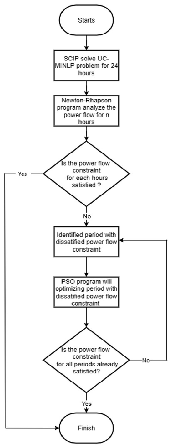
Figure 2. Flowchart of UC-OPF program.

The program begins by obtaining an initial solution for the UC and power flow optimization through a Mixed-Integer Nonlinear Programming (MINLP) approach applied to the UC model over a 24-h period. This process is implemented using the SCIP solver via the PySCIPOpt 5.6.0 library in Python 3.10.9. The optimal solution produced by SCIP is subsequently evaluated in terms of power flow feasibility through a Newton–Raphson-based analysis. If no power flow constraints are violated, the solution is considered optimal and the program terminates. However, if any violations of power flow constraints are detected, the program identifies the specific hours in which such violations occur. Optimization is then continued using PSO exclusively for those hours with constraint violations. The iterative process involving PSO optimization and Newton–Raphson power flow analysis is repeated until all violations are resolved and a fully feasible and optimal solution is achieved

4.4. SCIP and PSO Parameters Setting

To ensure reproducibility and consistent performance of the proposed optimization framework, the key parameters for both the SCIP solver and the PSO algorithm are summarized in this section. For the UC stage, the SCIP solver is configured with a maximum solving time of 100 s, which provides a balance between computational efficiency and solution quality for the 24-h scheduling horizon.

For the PSO-assisted OPF stage, the algorithm parameters were selected based on preliminary tuning and prior experience to ensure reliable convergence. Several key parameters require careful adjustment for effective PSO performance. The selected parameters and their corresponding values are summarized in Table 6.

Table 6. PSO and NR parameter tuning.

Parameter	Value
Number of particles	300–900
PSO Maximum iteration	10–15
NR maximum iteration	7
Inertia weight (ω)	0.7
Cognitive coefficient (c1)	1.5
Social coefficient (c2)	1.5

The PSO algorithm parameters used in this study are summarized in Table 6. The number of particles and maximum iterations are adjusted according to the load scaling scenario to ensure sufficient exploration of the solution space and convergence to high-quality solutions. For scenarios with larger system loads or more variability, a higher number of particles (up to 900) or iterations (up to 15) may be employed, whereas smaller or less variable scenarios can be effectively optimized with fewer particles (around 300) and iterations (10). This adaptive approach allows the algorithm to balance computational efficiency and solution accuracy across different operating conditions.

The inertia weight (ω) is set to 0.7, which provides a good balance between global exploration and local exploitation, preventing premature convergence while maintaining search efficiency. The cognitive coefficient (c1 = 1.5) and social coefficient (c2 = 1.5) are chosen to equally weight the influence of each particle’s personal best experience and the swarm’s global best solution, promoting convergence towards optimal regions of the solution space while avoiding stagnation in local minima. These parameter values are selected based on preliminary tuning and prior experience, ensuring reliable performance of the PSO-assisted Optimal Power Flow optimization under various system conditions.

In addition to the PSO algorithm parameters, the penalty weights assigned to various constraint violations are summarized in Table 7. These weights are crucial for guiding the optimization towards feasible and economically efficient solutions, ensuring that voltage limits, power balance, ramp-rate restrictions, and Newton–Raphson convergence requirements are properly enforced.

Table 7. 24- The Weight of Penalty for Every Penalty Type.

Penalty Type	Penalty Weight
Voltage Deviation Penalty (pV)	10,000
Active Power Generation Penalty (pP)	1000
Reactive Power Generation Penalty (pQ)	1000
Ramping Rate Violation Penalty (pRamp)	1000
Newton–Raphson Convergence Tolerance Penalty (pNR)	1,000,000

The values of penalty weight were determined based on a series of preliminary tests and trial-and-error experiments to ensure a balanced optimization between economic performance and operational feasibility. As a result, some penalty weights are set slightly higher than others to appropriately enforce constraint satisfaction.

In particular, the Newton–Raphson convergence penalty P_NR is assigned a very high value (1,000,000) compared to the other penalties. This is necessary because it directly validates the feasibility of each candidate solution: any particle that fails to converge in the power flow calculation represents an infeasible operating point, which must be strongly penalized to prevent the algorithm from considering invalid solutions.

Meanwhile, the weights for voltage deviation, active power mismatch, reactive power mismatch, and ramping violations are relatively lower but still significant, guiding the PSO to find solutions that respect operational limits while optimizing the total generation cost.

5. Results

5.1. UC with Load Flow Scheduling Results

The UC schedule obtained from the MINLP optimization is first presented to illustrate the on/off status and preliminary generation levels of each thermal and PHS unit over the 24-h scheduling horizon. This schedule provides the foundation for system operation and serves as the input for subsequent load flow analysis.

Following the UC stage, a Newton–Raphson (NR) load flow calculation is performed to evaluate the actual power generation, reactive power dispatch, bus voltages, and system losses resulting from the scheduled generator commitments. Table 8 and Table 9 summarize both the UC-derived generator schedule and the corresponding generation levels after load flow adjustment, highlighting the impact of network constraints on the realized dispatch. This comparison ensures that the UC schedule produces a feasible operating point and allows identification of any necessary adjustments to maintain voltage and power balance within permissible limits.

Table 8. Generator Configuration from UC.

Generator (Bus)						PV (MW)	PHS (MW)	Total Load (MW)	Cost ($)
Slack	1	12	21	22	26
36.4	48.75	9.12	19.65	9.12	12.36			135.40	411.31
35.3	47.49	8.24	19.3	8.24	9.72			128.30	345.94
34.88	47.01	7.91	19.16	7.91	8.71			125.57	336.65
35.01	47.15	8.01	19.2	8.01	9.01			126.39	339.43
35.47	47.68	8.38	19.35	8.38	10.13			129.40	349.67
33.23	45.13	6.59	18.64	6.59	4.76			114.93	300.85
30.76	42.3	4.61	17.84	4.61	0.1	2.4		102.64	252.53
30.48	41.98	4.39	17.75	4.39	0.1	8.2		107.28	248.93
30.86	42.41	4.68	17.87	4.68	0.1	26.1		126.67	253.81
32.01	43.73	5.61	18.24	5.61	1.82	41.8		148.78	274.71
32.62	44.42	6.1	18.44	6.1	3.28	54.2		165.16	287.68
33.64	45.59	6.91	18.76	6.91	5.73	57.7		175.26	309.59
32.35	44.11	5.88	18.35	5.88	2.63	77.3		186.45	281.89
31.56	43.21	5.25	18.1	5.25	0.74	85.9		190.00	265.20
34.25	46.29	7.4	18.96	7.4	7.21	64.9		186.45	322.94
35.88	48.15	8.7	19.48	8.7	11.1	51.4		183.45	358.67
38.31	50.93	10.65	20.26	10.65	16.93	29.7		177.44	413.39
40.36	53.27	12.29	20.92	12.29	21.85	19.2		180.17	460.75
43.26	56.59	14.61	21.84	14.61	28.81			185.63	529.60
43.47	56.83	14.78	21.91	14.78	29.31		6.32	186.45	534.64
43.12	56.42	14.5	21.8	14.5	28.47			178.81	526.16
41.64	54.73	13.31	21.33	13.31	24.92			169.25	490.85
40.25	53.14	12.2	20.88	12.2	21.58			160.24	458.08
38.3	50.92	10.64	20.26	10.64	16.92			147.69	413.24
Total								3717.8	8771.14

Table 9. Generator configuration from UC with load flow analysis.

Generator (Bus)						PV (MW)	PHS (MW)	Total Load (MW)	Cost ($)
Slack	1	12	21	22	26
38.03	48.75	9.12	19.65	9.12	12.36			137.03	420.98
36.81	47.49	8.24	19.30	8.24	9.72			129.81	351.11
36.33	47.01	7.91	19.16	7.91	8.71			127.03	341.63
36.48	47.15	8.01	19.20	8.01	9.01			127.86	344.47
36.99	47.68	8.38	19.35	8.38	10.13			130.92	354.91
34.52	45.13	6.59	18.64	6.59	4.76			116.23	305.21
31.85	42.30	4.61	17.84	4.61	0.10	2.43		103.75	256.12
31.61	41.98	4.39	17.75	4.39	0.10	8.19		108.41	252.57
32.67	42.41	4.68	17.87	4.68	0.10	26.06		128.47	259.72
35.16	43.73	5.61	18.24	5.61	1.82	41.76		151.93	285.24
37.26	44.42	6.10	18.44	6.10	3.28	54.19		169.79	303.45
38.94	45.59	6.91	18.76	6.91	5.73	57.70		180.55	327.87
40.43	44.11	5.88	18.35	5.88	2.63	77.25		194.53	309.81
41.06	43.21	5.25	18.10	5.25	0.74	85.89		199.50	297.99
40.73	46.29	7.40	18.96	7.40	7.21	64.93		192.92	345.58
40.82	48.15	8.70	19.48	8.70	11.10	51.42		188.37	376.08
41.47	50.93	10.65	20.26	10.65	16.93	29.71		180.61	424.77
43.20	53.27	12.29	20.92	12.29	21.85	19.19		183.01	471.17
46.09	56.59	14.61	21.84	14.61	28.81			188.45	540.28
45.10	56.83	14.78	21.91	14.78	29.31		6.32	189.03	540.79
45.78	56.42	14.50	21.80	14.50	28.47			181.48	536.24
44.05	54.73	13.31	21.33	13.31	24.92			171.65	499.75
42.40	53.14	12.20	20.88	12.20	21.58			162.41	465.98
40.18	50.92	10.64	20.26	10.64	16.92			149.56	419.92
Total								3793.7	9031.64

Table 8 and Table 9 summarize the generator configurations obtained from the UC stage and after performing load flow analysis, respectively, over a 24-h scheduling horizon. The UC results in Table 8 represent the initial generation schedule derived directly from the MINLP-based optimization, while Table 9 presents the adjusted generation outputs after applying the Newton–Raphson load flow to ensure network feasibility and power balance at every bus.

Based on Table 8 and Table 9, slight adjustments in the generation dispatch of all units can be observed after incorporating the load flow analysis. These variations occur because the power flow algorithm redistributes active and reactive power to satisfy nodal balance equations and voltage magnitude constraints. Notably, the Slack bus shows a consistent increase in output compared to the original UC results. This behavior occurs because the Slack generator is responsible for compensating transmission and transformation losses within the system, ensuring that total generated power matches the total load plus losses.

Consequently, the total system demand (load) increased slightly—from 3717.8 MW in the UC results to 3793.7 MW after load flow—reflecting the real power losses in the network. This additional demand leads to a corresponding rise in total generation cost, from $8771.14 to $9031.64. The difference represents the economic impact of real power losses that must be supplied by the committed units through the Slack bus. Overall, the post–load flow configuration in Table 10 represents a more realistic operating condition of the power system, as it accounts for both network constraints and physical losses, ensuring feasible and stable operation under the UC-defined schedule.

Table 10. Penalty summary of constraint violations in load flow results.

Hours	pV	pQ	pP	pRamp	pNR
1	-	-	-	-	-
2	-	-	-	-	-
3	-	-	-	-	-
4	-	-	-	-	-
5	-	-	-	-	-
6	-	-	-	-	-
7	-	[24, 0.21]	-	-	-
8	-	-	[24, 7.32 × 10−5]	-	-
9	-	-	[24, 0.001027]	-	-
10	-	-	-	-	-
11	-	-	-	-	-
12	-	-	-	-	-
13	-	-	-	-	-
14	-	-	[24, 0.001]	-	-
15	-	-	-	-	-
16	-	-	-	-	-
17	-	-	-	-	-
18	-	-	[24, 0.00219]	-	-
19	-	-	-	-	-
20	-	[5, 56.2]	-	-	-
21	-	-	-	-	-
22	-	-	-	-	-
23	-	-	-	-	-
24	-	-	-	-	-

After validating the load flow results, several constraint violations were detected across different operating parameters. These include voltage deviation (pV), active and reactive power mismatches (pP, pQ), ramp rate violation (pRamp), and Newton–Raphson convergence penalty (pNR). The summarized results in the following table illustrate the magnitude of each violation over the 24-h scheduling period, highlighting hours with greater operational difficulty due to varying load levels and PHS activity.

Table 10 summarizes the constraint violations that occurred during the 24-h UC–load flow simulation with PHS operation. Most hours exhibit no violations, indicating that the committed generation schedule generally satisfies power balance and voltage constraints. However, a few exceptions are observed at specific hours and buses.

Notably, minor active power mismatches (pP) and reactive power deviations (pQ) occur at Bus 24, which corresponds to the PV (solar) generator bus. These deviations arise from fluctuating solar output, which challenges the system’s ability to maintain precise power balance and voltage regulation. Additionally, a significant reactive power violation is detected at Bus 5, corresponding to the PHS unit, reflecting its dynamic operation during pumping and generating cycles.

These results highlight that while the unit commitment schedule ensures operational feasibility, certain conditions—particularly those involving renewable and storage dynamics—still cause constraint violations. Therefore, a further OPF stage is essential to refine generator dispatch and voltage control, ensuring that all system limits are fully satisfied.

5.2. OPF Dispatch Results

Following the unit commitment and preliminary load flow validation, the next stage involves the OPF analysis using the PSO–Newton Raphson framework. This stage aims to refine generator dispatch and bus voltage settings to minimize total generation cost while ensuring all operational and network constraints are satisfied. The OPF process adjusts the active and reactive power outputs of committed generators as well as the voltage magnitudes at PV buses, producing an optimized operating point for each hour within the scheduling horizon.

It is worth noting that the OPF analysis in this study employs an hourly temporal resolution, consistent with standard practice in UC and day-ahead OPF studies. This time step captures medium-term scheduling behavior rather than fast transient variations. Although solar generation may fluctuate within shorter intervals, the hourly average forecast adequately represents expected generation levels for each dispatch period. A finer temporal resolution (e.g., 5–15 min) would require a short-term or real-time OPF framework, which is beyond the current study’s scope but will be considered in future work. The detailed OPF dispatch results are presented in the following tables.

Table 11 presents the generator configuration obtained after applying the assisted OPF to the previously validated UC schedule. Compared to the post–load flow configuration in Table 10, noticeable adjustments occur in several generator outputs, particularly at the Slack and PV buses, as the OPF redistributes power generation to minimize total operating cost while maintaining system feasibility.

Table 11. Generator configuration with assisted OPF.

Generator (Bus)						PV (MW)	PHS (MW)	Total Load (MW)	Cost ($)
Slack	1	12	21	22	26
34.37	49.14	9.14	19.74	10.47	14.05			137.03	420.98
33.00	46.44	10.41	19.20	8.10	12.50			129.81	351.11
34.63	45.08	8.50	18.90	8.59	11.24			127.03	341.63
32.54	46.04	10.15	19.09	7.99	11.89			127.86	344.47
33.25	46.67	10.57	19.26	8.17	12.85			130.92	354.91
31.09	45.44	6.80	18.97	7.68	6.12			116.23	305.21
28.77	42.61	2.35	16.78	4.55	6.28	2.38		103.75	256.12
31.61	41.98	4.39	17.75	4.39	0.10	8.19		108.41	252.57
32.67	42.41	4.68	17.87	4.68	0.10	26.06		128.47	259.72
33.27	43.90	4.94	18.16	7.81	2.05	41.71		151.93	285.24
35.28	43.76	4.73	18.85	7.67	4.73	54.19		169.79	303.45
37.63	44.98	5.60	19.14	7.88	7.01	57.70		180.55	327.87
31.55	48.13	5.22	19.41	7.78	4.26	77.13		194.53	309.81
33.22	47.06	8.23	18.07	3.76	1.93	85.69		199.50	297.99
38.17	48.55	12.08	18.60	8.35	1.16	64.90		192.92	345.58
37.70	47.39	9.14	18.87	8.35	14.96	51.41		188.37	376.08
39.82	49.62	10.70	20.26	10.26	20.05	29.71		180.61	424.77
43.16	53.06	12.32	20.92	12.29	21.98	19.19		183.01	471.17
44.63	56.72	16.87	22.18	15.40	26.60			188.45	540.28
50.05	63.08	21.65	23.63	18.29	6.32		6.32	189.03	540.79
44.01	55.33	15.58	22.13	14.68	29.58			181.48	536.24
39.13	52.90	14.86	22.56	14.63	27.31			171.65	499.75
39.42	52.52	12.88	21.15	12.43	23.88			162.41	465.98
36.40	51.82	10.57	20.97	11.04	18.63			149.56	419.92
Total								3786	9016.05

As shown in the Table 11, the total generation cost decreases from $9031.64 (after UC with load flow) to $9016.05 after OPF optimization, indicating a more efficient power allocation. Similarly, the total system load slightly reduces from 3793.7 MW to 3786 MW, reflecting the mitigation of network losses through improved reactive power and generation scheduling. The smaller overall load demand implies reduced transmission losses within the network, as the OPF effectively fine-tunes generator dispatch to minimize unnecessary power flow stress and losses.

While these results suggest improved efficiency and cost reduction, further assessment is necessary to determine whether all operational constraints are fully satisfied. The following table presents a detailed analysis of the constraint violations observed during the OPF-assisted operation.

Table 12 presents the summary of constraint violations obtained from the OPF-assisted results. As shown, no violations were detected across all categories—including voltage deviation (pV), active power mismatch (pP), reactive power mismatch (pQ), ramping rate (pRamp), and Newton–Raphson convergence penalty (pNR)—throughout the 24-h scheduling horizon.

Table 12. Penalty summary for constraint violations in load flow results after OPF implementation.

Hours	pV	pQ	pP	pRamp	pNR
1	-	-	-	-	-
2	-	-	-	-	-
3	-	-	-	-	-
4	-	-	-	-	-
5	-	-	-	-	-
6	-	-	-	-	-
7	-	-	-	-	-
8	-	-	-	-	-
9	-	-	-	-	-
10	-	-	-	-	-
11	-	-	-	-	-
12	-	-	-	-	-
13	-	-	-	-	-
14	-	-	-	-	-
15	-	-	-	-	-
16	-	-	-	-	-
17	-	-	-	-	-
18	-	-	-	-	-
19	-	-	-	-	-
20	-	-	-	-	-
21	-	-	-	-	-
22	-	-	-	-	-
23	-	-	-	-	-
24	-	-	-	-	-

This complete elimination of penalties as shown in Table 12 confirms that the second-stage OPF dispatch not only corrects all mismatch and voltage deviation issues observed in the previous UC–load flow stage but also enhances the accuracy and reliability of the overall optimization process. In particular, the active power mismatch penalty (pP) values, which appeared in the UC stage (Table 10), were entirely removed after OPF optimization. This demonstrates that the OPF procedure effectively refines, rather than degrades, the active and reactive power balance achieved by the UC results—thereby ensuring both numerical convergence and operational feasibility of the system.

Compared to the earlier UC with load flow results (Table 11), where several violations were observed at PV (bus 24) and PHS (bus 5) locations, the OPF successfully mitigated these issues by optimally adjusting generator dispatch and reactive power support. This indicates that the optimization effectively restored operational feasibility, particularly at buses connected to renewable sources that previously exhibited voltage and power mismatch problems.

Overall, the elimination of all constraint violations demonstrates that the PSO-assisted OPF not only reduces operating costs and network losses but also ensures stable and feasible operation of both conventional and renewable generation units across the scheduling period.

It should be noted that the percentage of optimal solutions obtained from the first (UC) and second (OPF) stages cannot be explicitly quantified, as these two optimization layers serve different purposes and operate under distinct domains. The UC stage focuses on economic commitment and dispatch based on active power and operational limits, while the assisted OPF enforces complete power flow feasibility, including reactive power, voltage, and transmission line constraints. Consequently, the OPF does not represent a proportional “improvement” over UC in percentage terms but ensures that the UC-based schedule becomes technically feasible within the network.

During the redispatch process in the OPF stage, the total generation cost slightly increases relative to the pure UC solution due to the inclusion of network and voltage constraints. Specifically, the total generation costs were 8771.14 for the UC stage, 9031.64 for the UC with load flow, and 9016.05 after the assisted OPF, demonstrating that the OPF adjustment yields a technically feasible and economically consistent final solution with minimal cost deviation.

5.3. Voltage Profile

The voltage profile analysis aims to verify that the OPF redispatch maintains acceptable voltage levels across the system. Overall, both the pre- and post-OPF results show that all bus voltages remain within the standard operational limits, indicating that the optimization process does not degrade network stability.

However, a localized deviation was observed during hour 20 at the PHS bus (bus 5), where a reactive power violation had been previously detected in the load flow results. This behavior was mainly caused by the bidirectional power exchange of the pumped-hydro storage unit, which momentarily affected the reactive support around its connection point. After the OPF adjustment, the voltage at this bus was successfully stabilized within acceptable limits, confirming the effectiveness of the optimization in mitigating reactive power-related disturbances.

To further illustrate this condition, Figure 3 compares the bus voltage magnitudes before and after OPF during hour 20 that representing one of the peak-load periods. The post-OPF profile demonstrates improved voltage uniformity, particularly around the PHS-connected node.

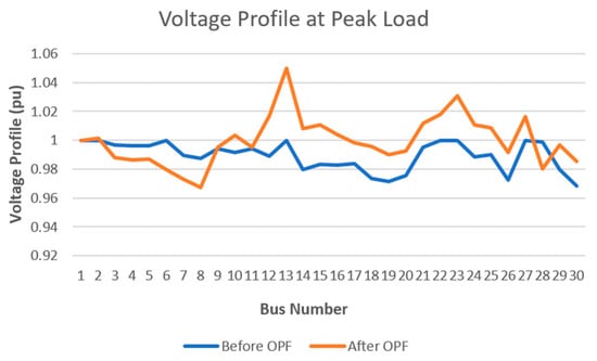
Figure 3. Voltage comparison in peak load.

While the overall voltage pattern across the 30 buses does not follow a consistent trend as shown in Figure 3, some buses experience slight increases and others slight decreases—the OPF redispatch effectively stabilizes the system. In particular, the voltage at the PHS-connected bus (bus 5), which previously experienced a reactive power violation, is restored to within acceptable limits. This localized improvement highlights the ability of OPF to mitigate voltage deviations caused by dynamic storage operations, while maintaining overall system voltages within standard operational ranges.

5.4. Multi-Scenario Analysis

This section presents a comprehensive analysis of the power system operation under multiple load scenarios, ranging from 50% to 150% of the base case demand. The primary objective is to evaluate the performance and flexibility of the integrated UC and OPF framework across varying system conditions.

• Voltage Comparison Before and After OPF

To evaluate the impact of OPF on network voltage performance, the bus voltage magnitudes under different load-scaling conditions are analyzed. The voltage profiles at 50%, 75%, 125%, and 150% loading conditions are shown in Figure 4, Figure 5, Figure 6 and Figure 7, respectively. Furthermore, a comparison of voltage profiles without OPF is presented in Figure 8, while the voltage profiles after applying OPF are illustrated in Figure 9. These results demonstrate the effectiveness of the OPF stage in correcting voltage deviations across the system.

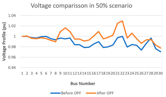
Figure 4. Voltage profile for system with 50% load scaling.

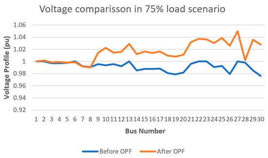
Figure 5. Voltage profile for system with 75% load scaling.

Figure 6. Voltage profile for system with 125% load scaling.

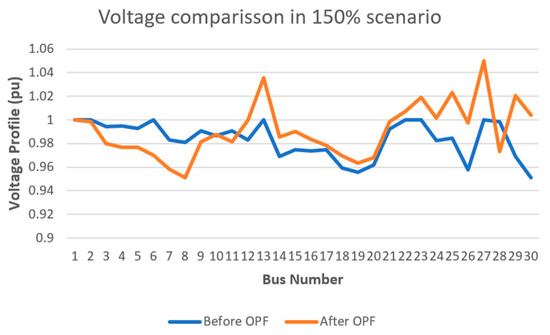
Figure 7. Voltage profile for system with 150% load scaling.

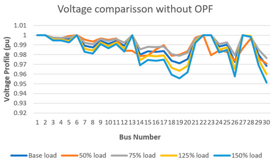
Figure 8. Voltage profile comparison without OPF.

Figure 9. Voltage profile comparison after OPF implementation.

The comparison of voltage profiles at peak-load conditions across various load scaling scenarios highlights the effectiveness of the OPF in maintaining bus voltages within acceptable operational limits. Before OPF, fluctuations were observed at several buses, particularly those connected to PHS and PV units, where voltages deviated from 1 pu due to reactive power imbalances. After OPF, voltage levels at all buses show improved stability, with values closer to 1 pu, indicating successful mitigation of voltage dips and surges even under scaled load conditions. Low-load scenarios (50–75% of peak) generally exhibit slightly higher voltages, whereas high-load scenarios (125–150%) display reduced voltages, which are significantly corrected after OPF. Minor deviations at some buses reflect their location relative to generation and load centers, illustrating the complex interactions of active and reactive power redistribution during peak-load operation.

b.

Power Loss Comparison

This section presents a comparison of total system real power losses over the 24-h scheduling horizon before and after applying the OPF, illustrating how the redispatch affects overall network losses throughout the day. The following table summarizes the total real power losses for the system over the 24-h scheduling horizon, comparing the losses computed from the initial UC schedule with those obtained after OPF optimization.

Table 13 summarizes the total real power losses over the 24-h horizon for various load scenarios, comparing the losses produced by the initial UC schedule with those obtained after applying the OPF. Overall, the OPF delivers a noticeable reduction in system losses for most scenarios. Under the base load condition, losses decrease from 75.42 MW to 68.22 MW, and at the highest loading condition (150% load), losses drop from 139.87 MW to 125.45 MW. A similar improvement is observed in the 50% load scenario. A slight increase occurs in the 75% load scenario, indicating that the OPF prioritizes satisfying generation limits, voltage constraints, and economic objectives over minimizing losses in this specific case. Nevertheless, the general trend shows that OPF redispatch enhances system efficiency across different loading levels.

Table 13. Power loss comparison.

Load Scenario	Before OPF	After OPF
Base load	75.42	68.22
50% load	43.74	41.74
75% load	57.61	57.90
125% load	103.94	91.05
150% load	139.87	125.45

Figure 10 illustrates the comparison of system power losses before and after OPF across all load scenarios. The figure clearly confirms the improvements indicated in Table 13, where OPF consistently reduces losses, particularly under higher loading conditions. The minor increase observed at 75% loading is also visible, reflecting the optimization trade-offs made to maintain feasibility and economic efficiency. Overall, the figure demonstrates that OPF redispatch contributes to improving network performance throughout the 24-h scheduling horizon.

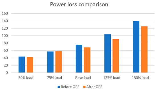
Figure 10. Power loss comparison with OPF.

c.

PHS impact on power system price

This section analyzes the PHS integration on the overall power system operation cost under various load-scaling conditions. The comparison is carried out between system performance with and without PHS to evaluate how energy storage contributes to economic efficiency and cost stability. By examining total operational costs at different load levels, the analysis aims to highlight the role of PHS in mitigating price fluctuations and enhancing the cost-effectiveness of power system operation in renewable-integrated environments.

Table 14 following with Figure 11 and Figure 12 shows the comparison of total generation costs between systems with and without Pumped Hydro Storage (PHS) for different load scaling scenarios. It can be observed that the presence of PHS slightly reduces the overall generation cost in all scenarios. For example, at 50% load, the system with PHS costs $2982.37 compared to $3021.36 without PHS, resulting in a difference of $38.99 or 1.29% relative to the base cost. As the load increases, the absolute cost difference grows modestly, but the relative difference decreases, reaching only 0.16% at 150% load. This indicates that PHS provides more noticeable economic benefits at lower load levels, while its impact becomes proportionally smaller as the system approaches peak demand. Overall, the results highlight the cost-saving potential of PHS integration across varying load conditions.

Table 14. Comparison of power system price between two systems.

Load Scale	With PHS ($)	Without PHS ($)	Price Difference ($)	Relative Difference to the Initial Price (%)
0.5×	2982.37	3021.36	38.99	1.29
0.75×	5697.31	5716.12	18.81	0.33
1.00×	8771.14	8790.68	19.54	0.22
1.25×	12,097.18	12,118.27	21.09	0.17
1.50×	15,660.12	15,684.64	24.52	0.16

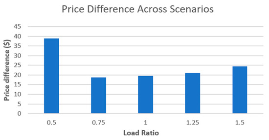
Figure 11. Price difference after PHS applied.

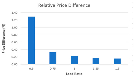
Figure 12. Relative difference with initial price (%).

6. Conclusions

This study presented the integration of OPF into the UC process to optimize generator scheduling while maintaining operational limits. The OPF-assisted UC effectively coordinated active and reactive power dispatch, ensuring feasible generator operation, improving system efficiency, and maintaining acceptable voltage and loss levels across the 24-h horizon.

Beyond the base case, a multi-scenario evaluation with load variations from 50% to 150% demonstrated the robustness of the proposed framework. In all scenarios, the OPF stage successfully restored feasibility by eliminating voltage violations observed in the UC-only solution and stabilizing bus voltages near 1 pu, regardless of loading severity. Power loss analysis showed that OPF reduced losses across most scenarios, with the most significant improvements occurring under high-load conditions.

The impact of Pumped Hydro Storage (PHS) was also assessed and found to provide consistent cost savings at all load levels, with the greatest relative benefit at lower loads. Although the absolute savings increased with demand, the proportional impact declined as the system approached peak load.

Overall, the integrated UC–OPF framework demonstrated high adaptability to varying demand conditions, effectively improving voltage stability, reducing losses, and enhancing economic performance—highlighting its practicality for renewable-integrated power system operation.

References

- Elomari, Y.; Norouzi, M.; Marín-Genescà, M.; Fernández, A.; Boer, D. Integration of Solar Photovoltaic Systems into Power Networks: A Scientific Evolution Analysis. Sustainability 2022, 14, 9249. [Google Scholar] [CrossRef]
- Nwaigwe, K.N.; Mutabilwa, P.; Dintwa, E. An overview of solar power (PV systems) integration into electricity grids. Mater. Sci. Energy Technol. 2019, 2, 629–633. [Google Scholar] [CrossRef]
- Fernandez, M.I.; Go, Y.I. Power management scheme development for large-scale solar grid integration. J. Electr. Syst. Inf. Technol. 2023, 10, 15. [Google Scholar] [CrossRef]
- Kabeyi, M.J.B.; Olanrewaju, O.A. Sustainable Energy Transition for Renewable and Low Carbon Grid Electricity Generation and Supply. Front. Energy Res. 2022, 9, 743114. [Google Scholar] [CrossRef]
- Osman, A.I.; Chen, L.; Yang, M.; Msigwa, G.; Farghali, M.; Fawzy, S.; Rooney, D.W.; Yap, P.-S. Cost, environmental impact, and resilience of renewable energy under a changing climate: A review. Environ. Chem. Lett. 2023, 21, 741–764. [Google Scholar] [CrossRef]
- Dada, M.; Popoola, P. Recent advances in solar photovoltaic materials and systems for energy storage applications: A review. Beni-Suef Univ. J. Basic Appl. Sci. 2023, 12, 66. [Google Scholar] [CrossRef]
- NREL. Best Research-Cell Efficiency Chart. Available online: https://www.nrel.gov/pv/cell-efficiency (accessed on 17 November 2025).
- Parthiban, R.; Ponnambalam, P. An Enhancement of the Solar Panel Efficiency: A Comprehensive Review. Front. Energy Res. 2022, 10, 937155. [Google Scholar] [CrossRef]
- Wu, C.; Zhang, X.-P.; Sterling, M. Solar power generation intermittency and aggregation. Sci. Rep. 2022, 12, 1363. [Google Scholar] [CrossRef]
- Di Leo, P.; Ciocia, A.; Malgaroli, G.; Spertino, F. Advancements and Challenges in Photovoltaic Power Forecasting: A Comprehensive Review. Energies 2025, 18, 2108. [Google Scholar] [CrossRef]
- Wesseh, P.K.; Chen, J.; Lin, B. Electricity price modeling from the perspective of start-up costs: Incorporating renewable resources in non-convex markets. Front. Sustain. Energy Policy 2023, 2, 1204650. [Google Scholar] [CrossRef]
- Harker Steele, A.J.; Burnett, J.W.; Bergstrom, J.C. The impact of variable renewable energy resources on power system reliability. Energy Policy 2021, 151, 111947. [Google Scholar] [CrossRef]
- Ali, M.B.; Kazmi, S.A.A.; Khan, Z.A.; Altamimi, A.; Alghassab, M.A.; Alojaiman, B. Voltage Profile Improvement by Integrating Renewable Resources with Utility Grid. Energies 2022, 15, 8561. [Google Scholar] [CrossRef]
- Kim, D.; Kim, H.; Won, D. Operation Strategy of Shared ESS Based on Power Sensitivity Analysis to Minimize PV Curtailment and Maximize Profit. IEEE Access 2020, 8, 197097–197110. [Google Scholar] [CrossRef]
- Emmanuel, M.; Giraldez, J.; Gotseff, P.; Hoke, A. Estimation of solar photovoltaic energy curtailment due to volt–watt control. IET Renew. Power Gener. 2020, 14, 640–646. [Google Scholar] [CrossRef]
- Kim, Y.; Son, B.; Kim, S.H. Operation Planing and Capacity Calculation of Energy Storage Systems Considering Curtailment of Renewable Energy. J. Korean Sol. Energy Soc. 2023, 43, 1–12. [Google Scholar] [CrossRef]
- Adeyinka, A.M.; Esan, O.C.; Ijaola, A.O.; Farayibi, P.K. Advancements in hybrid energy storage systems for enhancing renewable energy-to-grid integration. Sustain. Energy Res. 2024, 11, 26. [Google Scholar] [CrossRef]
- Topalović, Z.; Haas, R.; Ajanović, A.; Sayer, M. Prospects of electricity storage. Renew. Energy Environ. Sustain. 2023, 8, 2. [Google Scholar] [CrossRef]
- Singh, B.; Knueven, B.; Watson, J.-P. Modeling flexible generator operating regions via chance-constrained stochastic unit commitment. Comput. Manag. Sci. 2020, 17, 309–326. [Google Scholar] [CrossRef]
- Vasiyullah, S.F.S.; Bharathidasan, S.G. Profit Based Unit Commitment of Thermal Units with Renewable Energy and Electric Vehicles in Power Market. J. Electr. Eng. Technol. 2021, 16, 115–129. [Google Scholar] [CrossRef]
- Wuijts, R.H.; van den Akker, M.; van den Broek, M. Effect of modelling choices in the unit commitment problem. Energy Syst. 2024, 15, 1–63. [Google Scholar] [CrossRef]
- Li, Z.; Yin, H.; Wang, P.; Gu, C.; Wang, K.; Hu, Y. A fast linearized AC power flow-constrained robust unit commitment approach with customized redundant constraint identification method. Front. Energy Res. 2023, 11, 1218461. [Google Scholar] [CrossRef]
- Park, H. A Unit Commitment Model Considering Feasibility of Operating Reserves under Stochastic Optimization Framework. Energies 2022, 15, 6221. [Google Scholar] [CrossRef]
- Tuncer, D.; Kocuk, B. An MISOCP-Based Decomposition Approach for the Unit Commitment Problem with AC Power Flows. In IEEE Transactions on Power Systems; IEEE: New York, NY, USA, 2022; pp. 1–12. [Google Scholar] [CrossRef]
- Mohammadi, S.; Bui, V.-H.; Su, W.; Wang, B. Surrogate Modeling for Solving OPF: A Review. Sustainability 2024, 16, 9851. [Google Scholar] [CrossRef]
- Risi, B.-G.; Riganti-Fulginei, F.; Laudani, A. Modern Techniques for the Optimal Power Flow Problem: State of the Art. Energies 2022, 15, 6387. [Google Scholar] [CrossRef]
- Sabo, A.; Ibrahim Kanya, K.; Shu’aibu, N.; Onyema, C.; Aliyu, A.; Tanko, H.; Kwasau, S. A Review of State-of-the-Art Techniques for Power Flow Analysis. J. Sci. Technol. Eng. Res. 2023, 4, 36–43. [Google Scholar] [CrossRef]
- Montero, L.; Bello, A.; Reneses, J. A Review on the Unit Commitment Problem: Approaches, Techniques, and Resolution Methods. Energies 2022, 15, 1296. [Google Scholar] [CrossRef]
- Bacci, T.; Frangioni, A.; Gentile, C.; Tavlaridis-Gyparakis, K. New Mixed-Integer Nonlinear Programming Formulations for the Unit Commitment Problems with Ramping Constraints. Oper. Res. 2024, 72, 2153–2167. [Google Scholar] [CrossRef]
- Shaari, G.; Tekbiyik-Ersoy, N.; Dagbasi, M. The State of Art in Particle Swarm Optimization Based Unit Commitment: A Review. Processes 2019, 7, 733. [Google Scholar] [CrossRef]
- dos Santos, E.S.; Nunes, M.V.A.; Nascimento, M.H.R.; Leite, J.C. Rational Application of Electric Power Production Optimization through Metaheuristics Algorithm. Energies 2022, 15, 3253. [Google Scholar] [CrossRef]
- Yang, X.-S. Nature-inspired optimization algorithms: Challenges and open problems. J. Comput. Sci. 2020, 46, 101104. [Google Scholar] [CrossRef]
- Gad, A.G. Particle Swarm Optimization Algorithm and Its Applications: A Systematic Review. Arch. Comput. Methods Eng. 2022, 29, 2531–2561. [Google Scholar] [CrossRef]
- Mena, R.; Godoy, M.; Catalán, C.; Viveros, P.; Zio, E. Multi-objective two-stage stochastic unit commitment model for wind-integrated power systems: A compromise programming approach. Int. J. Electr. Power Energy Syst. 2023, 152, 109214. [Google Scholar] [CrossRef]
- Hussein, B.M.; Jaber, A.S. Unit commitment based on modified firefly algorithm. Meas. Control 2020, 53, 320–327. [Google Scholar] [CrossRef]
- Fusco, A.; Gioffrè, D.; Francesco Castelli, A.; Bovo, C.; Martelli, E. A multi-stage stochastic programming model for the unit commitment of conventional and virtual power plants bidding in the day-ahead and ancillary services markets. Appl. Energy 2023, 336, 120739. [Google Scholar] [CrossRef]
- Li, J.; Zhang, R.; Wang, H.; Liu, Z.; Lai, H.; Zhang, Y. Deep Reinforcement Learning for Optimal Power Flow with Renewables Using Graph Information. arXiv 2021, arXiv:2112.11461. [Google Scholar]
- Gholami Trojani, A.; Samiei Moghaddam, M.; Mohamadi Baigi, J. Stochastic Security-constrained Unit Commitment Considering Electric Vehicles, Energy Storage Systems, and Flexible Loads with Renewable Energy Resources. J. Mod. Power Syst. Clean Energy 2023, 11, 1405–1414. [Google Scholar] [CrossRef]
- Riaz, M.; Hanif, A.; Hussain, S.J.; Memon, M.I.; Ali, M.U.; Zafar, A. An optimization-based strategy for solving optimal power flow problems in a power system integrated with stochastic solar and wind power energy. Appl. Sci. 2021, 11, 6883. [Google Scholar] [CrossRef]
- Al-Roomi, A.R. 30-Bus System (IEEE Test Case). Available online: https://al-roomi.org/power-flow (accessed on 10 September 2025).
- Howlader, H.O.R.; Sediqi, M.M.; Ibrahimi, A.M.; Senjyu, T. Optimal thermal unit commitment for solving duck curve problem by introducing csp, psh and demand response. IEEE Access 2018, 6, 4834–4844. [Google Scholar] [CrossRef]
- Achterberg, T. SCIP: Solving constraint integer programs. Math. Program. Comput. 2009, 1, 1–41. [Google Scholar] [CrossRef]
- Bestuzheva, K.; Chmiela, A.; Müller, B.; Serrano, F.; Vigerske, S.; Wegscheider, F. Global optimization of mixed-integer nonlinear programs with SCIP 8. J. Glob. Optim. 2023, 91, 287–310. [Google Scholar] [CrossRef]
- Bolusani, S.; Besançon, M.; Bestuzheva, K.; Chmiela, A.; Dionísio, J.; Donkiewicz, T.; van Doornmalen, J.; Eifler, L.; Ghannam, M.; Gleixner, A.; et al. The SCIP Optimization Suite 9.0. arXiv 2024, arXiv:2402.17702. [Google Scholar] [CrossRef]
- Freitas, D.; Lopes, L.G.; Morgado-Dias, F. Particle Swarm Optimisation: A historical review up to the current developments. Entropy 2020, 22, 362. [Google Scholar] [CrossRef] [PubMed]
- Yavuz, A.; Celik, N.; Chen, C.-H.; Xu, J. A Sequential Sampling-based Particle Swarm Optimization to Control Droop Coefficients of Distributed Generation Units in Microgrid Clusters. Electr. Power Syst. Res. 2023, 216, 109074. [Google Scholar] [CrossRef]
- Kashyap, N.; Mishra, A. A discourse on metaheuristics techniques for solving clustering and semisupervised learning models. In Cognitive Big Data Intelligence with a Metaheuristic Approach; Elsevier: Amsterdam, The Netherlands, 2022; pp. 1–19. [Google Scholar] [CrossRef]
Disclaimer/Publisher’s Note: The statements, opinions and data contained in all publications are solely those of the individual author(s) and contributor(s) and not of MDPI and/or the editor(s). MDPI and/or the editor(s) disclaim responsibility for any injury to people or property resulting from any ideas, methods, instructions or products referred to in the content. |
© 2025 by the authors. Licensee MDPI, Basel, Switzerland. This article is an open access article distributed under the terms and conditions of the Creative Commons Attribution (CC BY) license (https://creativecommons.org/licenses/by/4.0/).