Abstract
The commonly used conversion coefficient for natural infiltration rates (N) is derived from single-zone or low-rise building assumptions and therefore fails to account for the substantial pressure differences driven by building height and seasonal temperature variations. These induced pressure differences significantly impact on the variations in infiltration rates within high-rise buildings, particularly during heating and cooling seasons. Therefore, this study develops a floor-resolved methodology for deriving N in high-rise buildings under various seasonal conditions, through extending the effective leakage area (ELA) model and incorporating normalization procedures that reflect seasonal and environmental conditions. Application of this method to high-rise buildings in South Korea shows that both infiltration rates and N values at upper and lower floors exceed those near the neutral pressure level (NPL) by more than a factor of two under winter conditions. Moreover, the derived N values deviate substantially from the commonly assumed reference value of 20 and vary systematically with floor height and season. These findings indicate that using a uniform N value can lead to considerable errors in estimating infiltration and associated energy loads, underscoring the necessity of height- and climate-specific conversion coefficients for accurate energy performance assessment.
1. Introduction
Infiltration and exfiltration, driven by pressure differences across a building envelope, cause uncontrolled heating and cooling loads, leading to energy loss [1]. In multi-family residential high-rise buildings (MFRHBs), infiltration accounts for a significant portion of winter energy consumption [2,3] underscoring the importance of accurately assessing the building energy performance. Moreover, inaccurate estimation of the infiltration rate can lead to significant errors in both predicting energy consumption and appropriately sizing HVAC systems [4,5]. Ng et al. [6] reported that improving infiltration settings in EnergyPlus increased HVAC electricity use by 3% and heating gas consumption by 8%. Heibati et al. [7] likewise showed that different airtightness assumptions for the same building lead to significant variations in calculated heating and cooling design loads. These findings further indicate that infiltration and leakage across the building envelope present the significant influence on building energy performance and HVAC system operations. Furthermore, the NREL Strategy Guideline further noted that the combined adjustments to design conditions, envelope characteristics, duct characteristics, and ventilation–infiltration parameters can overestimate cooling loads by up to 161%, consequently resulting in oversized equipment, increased costs, and reduced part-load efficiency [8]. Therefore, it is essential to accurately estimate infiltration rates for code compliance and reliable HVAC design.
Since the infiltration rate is driven by the pressure difference () across the building envelope, its calculation requires a prior assessment of the envelope pressure distribution [9]. Airtightness performance indicators related to infiltration are commonly expressed as Cubic Meter per Hour at 50 Pa (CMH50), Air Change rate per Hour at 50 Pa (ACH50), and Effective Leakage Area (ELA), which are measured using pressurized or depressurized tests at a reference between the indoors and outdoors [10]. However, the actual indoor–outdoor is generally less than 10 Pa for low-rise detached houses [11,12], while it ranges from approximately 25 Pa to 30 Pa for high-rise buildings and depends on the building height [13]. Because the actual pressure difference acting on the envelope significantly differs from the 50 Pa reference pressure used in the pressurization-depressurization method, it is necessary to convert the measured flow rate at 50 Pa () to estimate the natural infiltration rate ().The conversion coefficient () is primarily used for this conversion and is defined as a dimensionless parameter representing the ratio between and . Currently, is widely recommended, mainly based on studies for low-rise buildings [14]. However, the natural infiltration rate varies with environmental parameters such as building characteristics, wind conditions, and indoor-outdoor temperature differences. Consequently, the uniform application of a single constant can introduce considerable errors into the analysis results. The validity and uncertainty associated with this coefficient have been subjects of continuous research [15,16,17,18,19,20]. For example, Turner et al. [20] evaluated the variability of under different meteorological conditions using an infiltration model; however, the study was limited to low-rise buildings and thus did not adequately account for the height-dependent characteristic of high-rise buildings. Unlike low-rise buildings, high-rise buildings exhibit a distinct vertical pressure gradient with height, which must be reflected in the analysis [21].
Simulation tools such as EnergyPlus and TRNSYS currently estimate infiltration rates using the single-zone method based on the Effective Leakage Area (ELA) concept [22]. However, this approach cannot accurately represent the floor-by-floor in high-rise buildings, as it does not sufficiently account for variations in height. Although commercial simulation programs and multi-zone network models can analyze infiltration, their practical application is often limited by the extensive input data required and the computational complexity involved [23]. Therefore, evaluating infiltration in high-rise buildings requires a simplified approach that incorporates the coefficient . This process involves calculating the average natural infiltration rate, which is obtained by normalizing existing data to determine representative value.
This study extends the conventional LBL model that is mainly applied for single-zone and low-rise buildings, which help evaluate natural infiltration in high-rise buildings. A calculation process is proposed to determine representative N values that reflect pressure variations associated with building height and seasonal meteorological conditions. This approach addresses the inherent limitations of the traditional single-zone model, providing a simplified and reliable framework for evaluating natural infiltration in high-rise buildings.
2. Theoretical Review
2.1. Characterization of the Conversion Coefficient
Due to the difference between the actual natural acting on a building and the reference of 50 Pa, converting the measured airflow rate is necessary for energy performance evaluation. In this context, Kronvall and Persily introduced a conversion coefficient called , which converts the airflow rate measured at 50 Pa into the corresponding natural infiltration rate. Initially, this coefficient was assigned a fixed value of 20. Equation (1) can estimate the natural infiltration rate by dividing the airflow rate measured at 50 Pa by 20, and it has become the most widely adopted method:
Equation (1) offers a straightforward method for estimating natural infiltration rates using measured airtightness data. Although the value of 20 is widely used as a rule of thumb across studies from different countries, it lacks rigorous academic validation, as it is based on generalized gas tracer test results from a limited set of buildings. Consequently, it does not account for variations in building characteristics or local meteorological conditions. Notably, this value is primarily applied in single-zone or low-rise buildings, such as residential dwellings. This limitation led to criticism that the method causes significant errors in predicting natural infiltration rates [24]. Subsequently, Meier [19] proposed an improved method that incorporates building and environmental conditions into the conventional conversion coefficient using the Lawrence Berkeley Laboratory (LBL) infiltration model, which is based on physical principles. In this approach, the final conversion coefficient is determined by multiplying a base value () by various correction coefficients (), as expressed in Equation (2):
where represents the base conversion coefficient, determined from an infiltration/exfiltration ratio distribution map, and denotes correction factors that account for environmental parameters such as building airtightness, height, and shielding effects. Compared with the previous model that used a fixed conversion coefficient of 20, this approach represents an improvement by accounting for the variability patterns of infiltration. Nevertheless, the in Sherman’s model is derived from a distribution map based on low-rise, detached houses in specific regions, which limits its applicability in high-rise buildings. However, due to the application of a single annual average value, it fails to represent actual seasonal variations, and other studies have also examined the variability of . These studies compared and analyzed the values derived from actual measurements with the conventional fixed value of [15,16,17,18,19,20,24,25,26]. Table 1 summarizes reported values from previous studies. The values derived from various studies, including Sherman’s, show a wide distribution, ranging from a minimum of 13 to a maximum of 58. Most of these studies primarily focused on low-rise, detached houses. Specifically, Lai et al. [25] measured the natural infiltration rate in high-rise residential buildings and calculated . However, the measurements were carried out only during the summer, when the indoor–outdoor temperature difference was less than , thereby limiting the study’s ability to fully capture the stack effect–the primary source of pressure differentials in high-rise buildings. In addition, Roberts et al. [18] reported that could significantly exceed 20 under certain environmental conditions, such as the value of 58 observed for a detached house during summer.

Table 1.
Values for N reported in the literature.
In summary, the existing studies largely focused on low-rise buildings and thus share a fundamental limitation: the inability to adequately account for the pressure distribution characteristic of high-rise buildings. Because greater building height amplifies the envelope pressure difference through the combined effects of stack and wind, applying values derived from low-rise buildings can significantly reduce the accuracy of infiltration rate predictions. Therefore, there is a clear necessity to derive a new applicable to high-rise buildings.
2.2. Natural Infiltration Calculation
As reviewed in Section 2.1, for high-rise buildings, it is essential to accurately determining the natural infiltration rate, which is converted from the 50 Pa pressurized flow rate through the suitable coefficient . Therefore, as a prerequisite step for a rational calculation of , it is necessary to review the theoretical foundations used to calculate natural infiltration rates. Methods for estimating the natural infiltration rate can be broadly classified into two categories: measurement-based and theory-based methods. The measurement-based method, such as the tracer gas technique, involves injecting a tracer gas into the target building, monitoring its concentration changes over time, and calculating the natural infiltration rate from the observed data. Although this approach has the advantage of accurately reflecting on-site conditions, it is time-consuming and costly. However, a single measurement is often insufficient to capture variations caused by weather conditions, and previous studies have suggested that a minimum temperature difference of approximately is required to adequately reflect the influence of temperature-driven effects [27]. Consequently, this method is limited in its ability to derive an that reflects a various meteorological condition and the distinct pressure distribution of each floor in a high-rise building. Building pressure is generated by the driving forces of wind and the stack effect. Thus, the theoretical equation for the natural infiltration rate is derived by combining the two flow components—the airflow induced by wind and the airflow induced by the stack effect—using the root-sum-square relationship, as shown in Equation (3). It should be noted that the exponent simply results from the root-sum-square formulation and does not represent a pressure exponent. This summation method is employed because the two driving forces—the stack effect (temperature) and wind effect—act independently, producing a non-linear airflow through the building envelope. Using a simple linear summation would result in a significant overestimation of the total flow rate [28]. Mechanical systems operating within a building can also alter the ΔP across the building envelope, thereby influencing the infiltration rate. However, including the ΔP caused by mechanical systems into the natural infiltration rate calculation often results in over- or underestimated results. Consequently, simulation tools such as EnergyPlus calculate mechanical ventilation as a separate airflow component, distinguishing it from natural infiltration. Therefore, it is general to consider only wind and the stack effects when calculating the natural infiltration rate.
The natural infiltration rate caused by each pressure component can be expressed using the ELA model through Equation (4), where the effective leakage area () used in the infiltration rate calculation is determined by Equation (5) [29]. The ELA model represents the leakage paths of the building envelope as a single, equivalent orifice area. Accordingly, in Equation (4) represents the average pressure difference across the envelope. The airflow area is determined using the measured flow coefficient () and pressure exponent (), while denotes the air density, and is the reference pressure, typically 4 Pa. The square-root term in Equation (4) originates from the orifice-flow formulation, which assumes a pressure exponent n of 0.5 under fully turbulent flow. Thus, it does not represent the actual leakage exponent. To reflect the non-fully turbulent behavior of real leakage, a corrected exponent n of 0.6 is applied in Equations (5) and (6), consistent with the standard ELA model. In his pioneering work applying the ELA model to calculation, Sherman [14] formulated (=/) by incorporating the stack and wind coefficient () through the relationship between and , following Equation (6).
The ELA model calculates based on the envelope pressure difference, and building energy analysis programs also employ single-zone infiltration calculation equations derived from the ELA model for low-rise buildings [22]. Although the ELA model can estimate the natural infiltration rate under various meteorological conditions, it assumes a uniform envelope pressure difference across the entire building or a single representative zone. Consequently, it may not be suitable for high-rise buildings, where pressure differences vary significantly from floor to floor due to height-dependent stack and wind effects. High-rise buildings exhibit distinct vertical pressure gradients at each floor, which fluctuate according to the position of the Neutral Pressure Level (NPL). Based on this review, both the conventional and the existing calculation methodologies—which assume a single-zone model—have inherent limitations when applied to high-rise buildings. Therefore, this study proposes a specific methodology for calculating that preserves the theoretical foundation of the ELA model while avoiding the complexity of full multi-zone analysis for practical simplification. In this approach, the ELA model is applied individually to each floor of the high-rise building, effectively capturing the pressure variations induced by floor-by-floor height differences.
3. Methodology for the Conversion Coefficient
The calculation of the conversion coefficient proposed in this study is based on the application of the existing ELA model, treating each floor as an independent single zone. In multi-unit high-rise residential buildings, each unit is inherently separated by a floor slabs, which allows each floor to be reasonably regarded as an individual zone. Consequently, this approach enables an analysis that incorporates the height-dependent pressure differences, which were not adequately reflected in the conventional ELA model. Figure 1 illustrates this conceptual distinction by comparing the traditional single-zone assumption with the proposed multi-floor framework. The figure highlights how the pressure distribution along the building height, including the neutral pressure level (NPL) and its vertical gradient, leads to different infiltration patterns at each floor.

Figure 1.
Conceptual comparison of the single-zone model for low-rise buildings and the proposed model for high-rise buildings.
It should be noted that the proposed model in this study is developed based on several fundamental assumptions to enhance simplification and computational efficiency. The geometric configuration of the target building is idealized as a two-dimensional (2D) rectangular domain, while air leakage paths through the envelope are represented using the equivalent orifice flow equation under the assumption of fully turbulent flow conditions. In addition, a single-zone modeling approach is applied to each floor, whereby the pressure difference is assumed to be uniformly distributed across the building envelope. The indoor–outdoor air density difference is also considered constant, implying that the stack-effect-induced pressure varies linearly with height. Figure 2 illustrates the process of deriving the final using the measured and . The procedure is further structured into five main steps: (1) Meteorological Data Processing and Normalization, (2) Selection of Representative Pressure Difference, (3) Preprocessing of Measured Airtightness Data, (4) Calculation of Natural Infiltration Rate, and (5) Derivation of Final Conversion Coefficient. The detailed explanations of each step are shown below.

Figure 2.
Flowchart for calculating conversion coefficient.
Step 1. Meteorological Data Processing and Normalization
To ensure the objectivity of the calculated natural infiltration rate, the meteorological data (outdoor temperature and wind speed) used in the analysis undergoes statistical verification through the Jarque–Bera Test. This test assesses the normality of the dataset, which determines whether the mean or median should be used as the representative value in subsequent calculations. The statistically verified meteorological data are then used as input for calculating the floor-by-floor pressure difference. The Jarque–Bera Test evaluates whether a dataset follows a normal distribution based on its skewness () and kurtosis (). When the meteorological data exhibit non-normality, the median is adopted instead of the mean, ensuring the robustness of the analysis. The Jarque–Bera Test statistic () is calculated as follows [30].
where is the number of data points. A smaller value indicates that the dataset is closer to a normal distribution, providing the criterion for selecting representative meteorological data. If the p-value of the test is less than the significance level, indicating non-normality, the median is used; otherwise, the mean is applied.
Before being used in the pressure calculation to derive , the collected meteorological data are aggregated at hourly, daily, and monthly intervals. Therefore, it is necessary to identify an appropriate representative time scale by comparing the error rates among different aggregation periods. This step aims to prevent from being biased toward a specific time interval and to ensure that it represents a stable long-term average. The calculation result from the smallest time unit (i.e., the dataset containing the highest number of observations) is set as the reference, and the error rate is compared with that of the next larger time unit to balance simplicity and accuracy. If the error rate is less than 5%, this indicates that the increase in the data measurement interval introduces only a minor error. In this case, the reference unit is updated to the next larger time interval, which contains fewer data points but represents a broader timescale. Conversely, if the error rate is 5% or greater, the error resulting from data reduction is considered significant, and the previous time interval is finalized as the representative unit. This iterative process continues until the optimal time interval for calculation is conclusively determined. The selection logic can be summarized as follows:
where denotes the statistically determined representative value (mean or median) of the meteorological variable (e.g., outdoor temperature or wind speed) for each interval, as determined from the normality assessment.
Step 2. Selection of Representative Pressure Difference
The meteorological data derived are used to calculate the pressure difference caused by the stack effect () and the wind pressure (). For evaluating the natural infiltration rate, only the magnitude of the pressure difference is considered.
- Calculation of Floor-Specific Pressure Difference
The varies linearly with building height relative to the NPL and is proportional to the height difference between the NPL and the target floor. For application in the ELA model, the on each floor is assumed to act as an average pressure difference applied at the floor’s center (). However, for the floor where the NPL is located, the acts in opposite directions simultaneously—negative (−) above and positive (+) below the NPL—centered at the NPL [21]. As illustrated in Figure 3, the representative pressure difference () for this floor is calculated as the weighted average of the magnitudes of the pressure differences, with each direction weighted according to its relative influence.

Figure 3.
Method for determining the representative pressure difference.
The for a typical floor that does not contain the NPL (denoted as ) is calculated using Equation (9), while that for the floor containing the NPL is determined using Equation (10):
where is the height of the floor center, obtained by subtracting half of the floor height () from the height from the ground to the ceiling of that floor (). denotes the height of the NPL. and represent the outdoor and indoor temperatures, respectively, and is obtained from meteorological data. Specifically, for the calculation of on the NPL floor—where the geometric mean of the pressure distribution is required— (the vertical distance from the floor bottom to the NPL) and (the distance from the NPL to the ceiling) are used. and represent the average pressure magnitudes in the lower and upper portions of the NPL floor, respectively. These values are then combined using a weighted average to determine the representative pressure for the NPL floor. The floor-by-floor wind pressure is determined by the wind speed at the corresponding height. Because its variation with height exhibits non-linear characteristics, the median is adopted as the representative value. This approach provides greater robustness than the mean, as wind-induced pressure variations can fluctuate sharply with height or be influenced by localized flow conditions. The wind pressure is calculated as follows:
where denotes the wind speed obtained from the meteorological agency. Because wind speed varies with the measurement environment, it must be adjusted to reflect the conditions at the building site. Therefore, to calculate the wind pressure acting on the building envelope, the boundary layer thickness () and the wind speed exponent () specified in ASHRAE are applied [31]. This process converts the reference wind speed from the meteorological agency into the actual wind speed at each corresponding floor height, which is then used to calculate the final wind pressure.
- Calculation of Representative Pressure Difference of Whole-Building
In energy simulation programs, a building’s infiltration rate is often represented as a single overall value by modeling the entire building as one zone, rather than modeling each dwelling unit separately [22]. Therefore, to derive a single representative N for the entire building, the pressure difference due to the stack effect () and wind pressure () were calculated using a model that treats the whole building as a single zone. The overall stack effect pressure distribution for the building is analogous to that of the NPL floor, as the NPL is typically located near the middle of the building height. Accordingly, is calculated, similar to Equation (10), by averaging the pressures in the upper and lower sections and then applying height-based weighting to determine the geometric mean. Similarly, is obtained by substituting the height variable in Equation (11) with the building’s mid-height, .
Step 3. Preprocessing Measured Airtightness Data
The final equation for depends on the pressure exponent obtained from the measured data. Data acquired through the pressurization-depressurization test at 50 Pa often contains outliers caused by temporary pressure fluctuations or measurement errors [32]. Therefore, an outlier remover process was applied to ensure the reliability and robustness of the derived building characteristic parameter. Since is calculated as the ratio of and , the flow coefficient cancels out in the final equation, making the accuracy of the pressure exponent critical. The Interquartile Range (IQR) method was employed for outlier detection [33], where data points outside the quartile-based boundaries are outliers and excluded from the analysis.
Step 4. Calculation of Natural Infiltration Rate
The natural infiltration rate is calculated based on the ELA equation to determine the individual airflow rates driven by pressure differences (). These two components are then combined into using the root-sum-square method (Equation (3)). To account for the leakage characteristics of each floor, the individual flow rates are computed using the pressure differences calculated for each floor (). The infiltration rates caused by the stack effect and wind are further adjusted using the stack parameter () and wind parameter () [29]. These parameters are introduced as reduction coefficients to compensate for the limitations of the single-zone ELA model, reflecting the non-uniform distribution of leakage across the building envelope and the complexity of an internal flow network. The following Equations (12)–(15) define the relationships with the leakage distribution parameters () and the shielding coefficient () proposed by Lawrence Berkeley Laboratory. It should be noted that the shown in Equation (15) represents the wind speed attenuation factor accounting for façade pressure effects, and the recommended moderate value of 0.25 is applied in this study [26]. Additionally, the square-root terms in Equations (12) and (14) originate from the orifice-flow formulation, which assumes a pressure exponent n of 0.5 under fully turbulent flow.
where represents the building’s shielding coefficient proposed by Lawrence Berkeley Laboratory [34]. The parameter R is defined as the ratio of the sum of the ceiling and floor leakage areas () to the total leakage area () of the indoor space. The parameter is defined as the ratio of the difference between the ceiling and floor leakage area () to the total leakage area. Because determining the exact leakage area of each surface in an actual building is practically difficult, an average approximation value of was applied to apartment buildings [35,36,37]. The parameter indicates the vertical asymmetry in leakage area caused by the stack effect. When , takes a value of when the ceiling leakage area () is dominant, and when the floor leakage area () is dominant. Assuming maximum vertical infiltration, a uniform value of was applied to all floors except the NPL floor.
Step 5. Derivation of Final Conversion Coefficient
Finally, , which reflects the floor-by-floor pressure difference variations, is derived as the ratio of the measured infiltration rate obtained from the pressurization–depressurization test to the natural infiltration rate calculated using the ELA model. The final equation is presented as Equation (16).
4. Application and Verification
To verify the practicality of the proposed methodology for calculating the conversion coefficient, the process was applied to a high-rise residential building in South Korea. The target building has 45 stories, with an average floor height of 3 m. Internal shaft temperatures and other necessary input data for pressure calculation were obtained from previous studies [31,38,39]. Table 2 summarizes the parameters and detailed information used for the application of the proposed methodology.
Table 2.
Data used in pressure difference calculation.
The results from the Jarque–Bera Test indicated that the measured wind speed and temperature data did not follow a normal distribution. Consequently, the median, which is less sensitive to outliers, was adopted as the representative value. In the time-scale analysis, hourly data was used for outdoor temperature due to its pronounced diurnal variation, whereas daily data was used for wind speed, given its smaller range of variation and to improve computational efficiency. Typically, a pressure exponent of 0.6 is employed in building air infiltration analyses [40]. This value was applied to calculate the natural infiltration rate and the conversion coefficient.
As shown in Figure 4, the minimum value of was observed near the NPL, which was assumed to be located at the building’s midpoint (23rd floor) in this study. This occurs due to the minimal indoor–outdoor pressure difference in this region. Conversely, the values exhibited a substantial increase, showing an inverse relationship with . The seasonal analysis indicated that the natural infiltration rate was generally higher in winter, when the driving force of the stack effect is stronger. The vertical variation of ranged from a minimum of 6.5 to a maximum of 27.9 in summer, and from 4.5 to 23.4 in winter. Notably, in winter, the value for the floors near the NPL and for the top/bottom floors differed by more than fivefold. This pronounced floor-by-floor variation clearly demonstrates that applying a single uniform N to represent the entire building can lead to substantial errors for individual floors.

Figure 4.
Vertical distribution of and N values.
However, as noted in the previous sections, a building’s energy performance is often evaluated using a single representative value for the entire structure. Therefore, it is necessary to determine a building-average conversion coefficient () based on the representative pressure value calculated for the whole building. Figure 5 presents the variation of NAvg across different building heights, using meteorological data from South Korea and a pressure exponent of 0.6. In particular, low-rise, mid-rise, and high-rise buildings correspond to 4-story (12 m), 20-story (60 m), and 45-story (135 m) buildings, respectively. The results indicate that the average for high-rise buildings was 8.8 in summer and 6.2 in winter. For mid-rise buildings, the values were 12.9 in summer and 9.3 in winter, while for low-rise buildings, they were 27.4 and 20.9, respectively. These results demonstrate that low-rise buildings exhibit values more than three times higher than those of high-rise buildings, confirming that varies significantly with the variation in building heights. Furthermore, the average values in summer and winter differed by approximately 20% was observed across all building types.
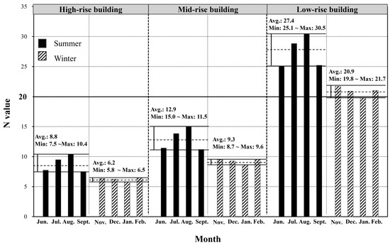
Figure 5.
Comparison of values by season and building height.
The preceding analysis of floor-specific and seasonal values focused on confirming the overall trend of variability in the conversion coefficient assuming a common pressure exponent of 0.6. To verify the distribution of under actual environmental conditions based on the proposed methodology, we analyzed airtightness data obtained from measurements conducted in South Korea. A total of 1175 individual dwelling units across 13 multi-family residential complexes were included in the analysis to derive an objective conversion coefficient representative of real conditions, and the summary of test samples is shown in Table 3.
Table 3.
Summary of Test Samples.
Prior to calculating the values using the representative pressure difference, a data preprocessing procedure was conducted. Figure 6 presents the box plots illustrating the distributions of the measured flow coefficient and the pressure exponent for all 1175 samples. As a result of the outlier removal process, a total of 1106 valid data points were selected from the 1175 initial measurement records. The final dataset exhibited a flow coefficient range of 31 to 167 (m3/(s·Pan)) and a pressure exponent range of 0.54 to 0.69.
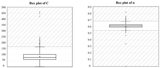
Figure 6.
Distribution of Airflow Coefficients () and Pressure Exponents ().
Figure 7 presents the conversion coefficient, derived from the measured airtightness data, as the Probability Density Function (PDF) for summer and winter conditions in Korea. The representative value, obtained through weighted averaging of the measured data, clearly demonstrates a significant dependence on building height. For low-rise buildings, ranged from 23 to 33 in summer, 21 to 30 in interseason, and 21 to 29 in winter. For mid-rise buildings, the ranges were from 10 to 16 in summer, 10 to 15 in interseason, and 8 to 12 in winter. High-rise buildings exhibited the lowest values, ranging from 7 to 11 in summer, 7 to 10 in interseason, and 5 to 8 in winter. As building height increased, not only did the overall values decrease, but the seasonal variation and range of also became narrower. Therefore, applying a conversion coefficient that appropriately reflects both climatic and height characteristics is essential for accurate energy performance evaluations. This finding supports the use of height-specific values in building energy simulations.
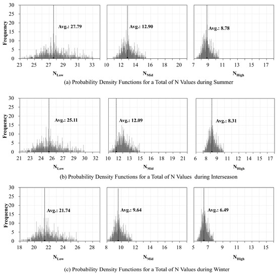
Figure 7.
Probability density function of the N values.
In addition, it should be noted that the values calculated for low-rise buildings were generally consistent with the previously published range of 20–30, as summarized in Table 1. Furthermore, research reports published by NYSERDA and the U.S. Department of Energy [41] indicated that the ratio of / for mid-rise residential buildings with 11–13 stories ranged from 7.9 to 9.25. This result aligns well with the value range (8–15.5) derived for mid-rise buildings in this study. Although the values for high-rise buildings are limited in the existing literature, the overall consistency between the derived values and previously reported results for low- and mid-rise buildings supports the validity and reliability of the proposed model.
5. Discussion and Limitations
This study proposed a methodology for estimating natural infiltration rates in high-rise buildings by accounting for variations in building height and seasonal conditions. The height- and climate-dependent N values derived in this manuscript offer practical applicability to conventional building energy assessment procedures, particularly those adopting monthly or simplified hourly calculation methods. Unlike the commonly applied fixed N value of 20—which is typically used for low-rise buildings and fails to account for height- or climate-related influences—the proposed N values incorporate the effects of building height, season, and climate. As a result, the approach substantially reduces the risk of overestimating or underestimating infiltration in high-rise buildings. By considering the dynamic characteristics of pressure differences driven by wind and stack effects, the method improves the accuracy of infiltration-related inputs in energy performance evaluation tools and enhances the reliability of estimated heating and cooling loads. Furthermore, the proposed methodology can be applied to high-rise buildings in various regions or countries, as long as the relevant meteorological data and airtightness databases are available. The assumed coefficients can also be adjusted based on the characteristics of the target building, enabling more accurate and context-specific evaluations.
However, several limitations should be acknowledged. The methodology is based on steady-state assumptions and simplified rectangular envelope geometries, and the N values were derived from representative meteorological datasets and average pressure distributions. Therefore, the influence of real-time measured pressure data on the distribution of N values could not be fully assessed. Additionally, although the reliability of the proposed N values was examined through comparisons with previously published data for low- and mid-rise buildings, direct comparisons between measured and calculated N values for high-rise buildings were not possible due to the lack of tracer-gas-based measurements for high-rise buildings. Moreover, representing infiltration using a single seasonal ACHn is appropriate for monthly or hourly evaluation procedures but cannot capture the temporal variability of wind and stack effects in dynamic pressure models. Future research should therefore include extensive field-based validation across a wider range of building types, envelope systems, and climate zones, and develop a broader N-value database to improve the generalizability and applicability of the proposed methodology for high-rise buildings.
6. Conclusions
This study developed a methodology for deriving the conversion coefficient (N) required to estimate natural infiltration rates in high-rise buildings. The proposed approach extends the Effective Leakage Area (ELA) method restructures it into a five-step procedure capable of incorporating floor-specific pressure difference variations. The procedure includes determining the driving pressure differences, normalizing relevant meteorological conditions, separating floor-by-floor and whole-building representative pressures, calculating the resulting infiltration rates, and deriving the corresponding N values. Application of the proposed methodology to an assumed high-rise building demonstrated that the variability of N increases markedly with larger indoor–outdoor temperature differences and building heights, even under constant wind speed. This finding confirms that applying a single uniform N value across all floors is inappropriate and may produce substantial floor-specific estimation errors.
Although the proposed method is based on a simplified airflow model and presents limitations for buildings with highly complex geometries, it offers practical advantages for both research and engineering applications. By requiring only fundamental inputs—such as building height, neutral pressure level, and basic meteorological data—it enables the estimation of natural infiltration rates without the need of complex multi-zone simulation process. This capability supports energy performance evaluations across entire high-rise buildings by capturing floor-specific discrepancies in heating and cooling loads. Considering the applied data types, this method can also be applied into various stages during the building lifecycle. During the building design and planning stage, through the application of assumed or experience parameters, the evaluated results can further guide the design and optimization of building energy systems. When integrated with real-time environmental data and actual building information during the building operation stage, it also provides a pathway for monitoring floor-by-floor infiltration behavior, offering potential applications in performance diagnostics and intelligent building management.
Furthermore, the proposed methodology can be extended to high-rise buildings of different heights and climatic regions, requiring only local meteorological data and measured airtightness characteristics. Broader application of the methodology across diverse building types will help refine the fixed parameters and improve its ability to represent real building conditions, thereby enhancing both its accuracy and practical relevance.
Author Contributions
Conceptualization, J.-h.J.; Methodology, S.L. and J.-h.J.; Data curation, S.L.; Writing—original draft preparation, S.L.; Writing—review and editing, S.-j.C. and J.J.; Supervision, J.-h.J. All authors have read and agreed to the published version of the manuscript.
Funding
This work was supported by an INHA UNIVERSITY Research Grant.
Data Availability Statement
The original contributions presented in the study are included in the article, and further inquiries can be directed to the corresponding author.
Conflicts of Interest
The authors declare no conflicts of interest.
References
- Hu, J.; Liu, Z.; Ma, G.; Zhang, G.; Ai, Z. Air Infiltration and Related Building Energy Consumption: A Case Study of Office Buildings in Changsha, China. J. Build. Eng. 2023, 74, 106859. [Google Scholar] [CrossRef]
- Meiss, A.; Feijó-Muñoz, J. The Energy Impact of Infiltration: A Study on Buildings Located in North Central Spain. Energy Effic. 2015, 8, 51–64. [Google Scholar] [CrossRef]
- Yoon, S.; Song, D.; Kim, J.; Lim, H. Stack-Driven Infiltration and Heating Load Differences by Floor in High-Rise Residential Buildings. Build. Environ. 2019, 157, 366–379. [Google Scholar] [CrossRef]
- Ng, L.C.; Emmerich, S.J.; Persily, A.K. An improved method of modeling infiltration in commercial building energy models. In Proceedings of the 2014 ASHRAE/IBPSA-USA Building Simulation Conference, Atlanta, GA, USA, 10–12 September 2014; pp. 308–315. [Google Scholar]
- Bae, Y.; Joe, J.; Lee, S.; Im, P.; Ng, L.C. Evaluation of Existing Infiltration Models Used in Building Energy Simulation. In Proceedings of the 17th IBPSA Conference, Bruges, Belgium, 1–3 September 2021; pp. 1085–1089. [Google Scholar]
- Ng, L.C.; Dols, W.S.; Emmerich, S.J. Evaluating Potential Benefits of Air Barriers in Commercial Buildings Using NIST Infiltration Correlations in EnergyPlus. Build. Environ. 2021, 196, 107783. [Google Scholar] [CrossRef] [PubMed]
- Heibati, S.; Maref, W.; Saber, H.H. Assessing the Energy, Indoor Air Quality, and Moisture Performance for a Three-story Building Using an Integrated Model, Part Three: Development of Integrated Model and Applications. Energies 2021, 14, 5648. [Google Scholar] [CrossRef]
- Burdick, A. Strategy Guideline: Accurate Heating and Cooling Load Calculations. In Building America Building Technologies Program Office of Energy Efficiency and Renewable Energy; U.S. Department of Energy: Washington, WA, USA, 2011; pp. 1–47. [Google Scholar]
- ASHRAE. Chapter 16—Ventilation and Infiltration. In 2017 ASHRAE Handbook—Fundamentals (SI Edition); ASHRAE: Atlanta, GA, USA, 2017. [Google Scholar]
- ISO 9972:2015; Thermal Performance of Buildings-Determination of Air Permeability of Buildings-Fan Pressurization Method. International Organization for Standardization: Geneva, Switzerland, 2015.
- World Health Organization. WHO Guidelines for Indoor Air Quality: Dampness and Mould; World Health Organisation: Copenhagen, Denmark, 2009; ISBN 9789289041683. [Google Scholar]
- Kalamees, T.; Kurnitski, J.; Jokisalo, J.; Eskola, L.; Jokiranta, K.; Vinha, J. Air Pressure Conditions in Finnish Residences. In Proceedings of the Clima 2007 WellBeing Indoors, Helsinki, Finland, 10–14 June 2007. [Google Scholar]
- Jo, J.H.; Lim, J.H.; Song, S.Y.; Yeo, M.S.; Kim, K.W. Characteristics of Pressure Distribution and Solution to the Problems Caused by Stack Effect in High-Rise Residential Buildings. Build. Environ. 2007, 42, 263–277. [Google Scholar] [CrossRef]
- Sherman, M.H. Estimation of Infiltration from Leakage and Climate Indicators. Energy Build. 1987, 10, 81–86. [Google Scholar] [CrossRef]
- Pasos, A.V.; Zheng, X.; Smith, L.; Wood, C. Estimation of the Infiltration Rate of UK Homes with the Divide-by-20 Rule and Its Comparison with Site Measurements. Build. Environ. 2020, 185, 107275. [Google Scholar] [CrossRef]
- Keig, P.; Hyde, T.; McGill, G. A Comparison of the Estimated Natural Ventilation Rates of Four Solid Wall Houses with the Measured Ventilation Rates and the Implications for Low-Energy Retrofits. Indoor Built Environ. 2016, 25, 169–179. [Google Scholar] [CrossRef]
- Pasos, A.V.; Zheng, X.; Gillott, M.; Wood, C.J. Comparison between Infiltration Rate Predictions Using the Divide-by-20 Rule of Thumb and Real Measurements. In Proceedings of the 40th AIVC Conference, Ghent, Belgium, 15–16 October 2019; pp. 420–429. [Google Scholar]
- Roberts, B.M.; Allinson, D.; Lomas, K.J. Evaluating Methods for Estimating Whole House Air Infiltration Rates in Summer: Implications for Overheating and Indoor Air Quality. Int. J. Build. Pathol. Adapt. 2023, 41, 45–72. [Google Scholar] [CrossRef]
- Meier, A. Infiltration: Just Ach 50 Divided by 20? Home Energy 1994, 11, 25–37. [Google Scholar]
- Turner, W.J.N.; Sherman, M.H.; Walker, I.S.; Walker, I.S. Infiltration as Ventilation: Weather-Induced Dilution. HVAC R. Res. 2012, 18, 1122–1135. [Google Scholar] [CrossRef]
- Park, S.Y.; Lee, D.S.; Ji, K.H.; Jo, J.H. Simplified Model for Estimating the Neutral Pressure Level in the Elevator Shaft of a Building. J. Build. Eng. 2023, 79, 107850. [Google Scholar] [CrossRef]
- EnergyPlus. EnergyPlusTM, Version 9.5.0. Documentation: Engineering Reference. US Department of Energy: Washington, DC, USA, 2021.
- Emmerich, S.; Dols, W.; Axley, J. Natural Ventilation Review and Plan for Design and Analysis Tools; US Department of Commerce, Technology Administration, National Institute of Standards and Technology: Gaithersburg, MD, USA, 2001. [Google Scholar]
- Jones, B.; Persily, A.; Sherman, M.H. The Origin and Application of Leakage-Infiltration Ratios. In Proceedings of the ASHRAE and AIVC IAQ, 2016, Alexandria, VA, USA, 12–14 September 2016. [Google Scholar]
- Lai, Y.; Ridley, I.A.; Brimblecombe, P. Air Change in Low and High-Rise Apartments. Urban Sci. 2020, 4, 25. [Google Scholar] [CrossRef]
- Johnston, D.; Stafford, A. Estimating the Background Ventilation Rates in New-Build UK Dwellings-Is N50/20 Appropriate? Indoor Built Environ. 2017, 26, 502–513. [Google Scholar] [CrossRef]
- Almeida, R.M.S.F.; Barreira, E.; Moreira, P. A Discussion Regarding the Measurement of Ventilation Rates Using Tracer Gas and Decay Technique. Infrastructures 2020, 5, 85. [Google Scholar] [CrossRef]
- Walker, I.S.; Wilson, D.J. Evaluating Models for Superposition of Wind and Stack Effect in Air Infiltration. Build. Environ. 1993, 28, 201–210. [Google Scholar] [CrossRef]
- Liddament, M.W. Air Infiltration Calculation Techniques-An Application Guide; Air Infiltration and Ventilation Centre: Berkshire, UK, 1986. [Google Scholar]
- Jarque, C.M.; Bera, A.K. A Test for Normality of Observations and Regression Residuals. Int. Stat. Rev. 1987, 55, 163–172. [Google Scholar] [CrossRef]
- ASHRAE. Chapter 24—Airflow Around Buildings. In 2017 ASHRAE Handbook—Fundamentals (SI Edition); ASHRAE: Atlanta, GA, USA, 2017. [Google Scholar]
- Mélois, A.; Carrié, F.R.; El Mankibi, M.; Moujalled, B. Uncertainty in Building Fan Pressurization Tests: Review and Gaps in Research. J. Build. Eng. 2022, 52, 104455. [Google Scholar] [CrossRef]
- Schwertman, N.C.; Owens, M.A.; Adnan, R. A Simple More General Boxplot Method for Identifying Outliers. Comput. Stat. Data Anal. 2004, 47, 165–174. [Google Scholar] [CrossRef]
- Sherman, M.H.; Grimsrud, D.T. Measurement of Infiltration Using Fan Pressurization and Weather Data. In Proceedings of the First Air Infiltration Centre Conference, Windsor, UK, 6–8 October 1980. [Google Scholar]
- Lozinsky, C.H.; Touchie, M.F. Quantifying Suite-Level Airtightness in Newly Constructed Multi-Unit Residential Buildings Using Guarded Suite-Level Air Leakage Testing. Build. Environ. 2023, 236, 110273. [Google Scholar] [CrossRef]
- Shin, H.K.; Jo, J.H. Air Leakage Characteristics and Leakage Distribution of Dwellings in High-Rise Residential Buildings in Korea. J. Asian Archit. Build. Eng. 2013, 12, 87–92. [Google Scholar] [CrossRef]
- Li, X.; Zhou, W.; Duanmu, L. Research on Air Infiltration Predictive Models for Residential Building at Different Pressure. Build. Simul. 2021, 14, 737–748. [Google Scholar] [CrossRef]
- Ji, K.H.; Choi, S.J.; Jo, J.H. Field Study on Impact of Mechanical Pressurization on Pressure Distribution in High-Rise Buildings. Buildings 2023, 13, 3039. [Google Scholar] [CrossRef]
- Hassina, B.; Samıra, L.E.B. Thermal Comfort Examination of the Staircase as a Transitional Space between the Dwelling and the External Environment. Kocaeli Üniversitesi Mimar. Ve Yaşam Dergisi. 2024, 9, 571–596. [Google Scholar] [CrossRef]
- Liddament, M.W. The Calculation of Wind Effect on Ventilation. ASHRAE Trans. 1988, 94. [Google Scholar]
- Henderson, H.; Harley, B. Infiltration Guidance for Buildings at Design Conditions—For the NYS Clean Heat Program; NYSERDA Report 07-13; New York State Energy Research & Development Authority (NYSERDA): Albany, NY, USA, 2022. [Google Scholar]
Disclaimer/Publisher’s Note: The statements, opinions and data contained in all publications are solely those of the individual author(s) and contributor(s) and not of MDPI and/or the editor(s). MDPI and/or the editor(s) disclaim responsibility for any injury to people or property resulting from any ideas, methods, instructions or products referred to in the content. |
© 2025 by the authors. Licensee MDPI, Basel, Switzerland. This article is an open access article distributed under the terms and conditions of the Creative Commons Attribution (CC BY) license (https://creativecommons.org/licenses/by/4.0/).