Abstract
In this paper we present the development of an energy and power system modelling, simulation, and analysis (ePowerSim.jl) package in Julia programming language. ePowerSim.jl is designed to present a uniform data interface for static, quasi-static, dynamic analysis, as well as network operation optimisation. It provides a co-simulation framework for the further development and experimentation of various types of models of electric power systems components or abstract entities that have mathematical formalism or data representation. ePowerSim.jl makes extensive use of cutting edge packages such as DifferentialEquations.jl, Dataframes.jl, NamedTupleTools.jl, Helics.jl, ForwardDiff.jl, JuMP.jl, and BifurcationKit just to mention a few in the Julia ecosystem. Models of synchronous generator, synchronous condenser, excitation systems, and governors developed in the package were used to model IEEE 9 bus and IEEE 14 bus test networks and subsequently validated by a real-time digital simulator of electric power systems (RTDS). The results obtains for static and dynamic models simulation in ePowerSim.jl show a close match with a simulation of the same system in RTDS. A maximum error of pu and pu were obtained for steady states and transient state respectively. Similarly, a maximum deviation of pu was obtained during validation for voltage magnitude during transient state at buses in the network.
1. Introduction
Static, quasi-static, and dynamic models with an appropriate simulation environment play an important role in having good insight into the planning and operation of electric power systems. In recent times, various open-source applications and packages have been developed by researchers to open up the electric power systems modelling and simulation domain. The electric power systems modelling and simulation space is traditionally dominated by commercial applications such as DigSilent, PSS, ETAP, PSCAD, PowerWorld and MATLAB. In cases where there is a need for validation, the coordination of protection devices, and hardware-in-the-loop, platforms that have real-time simulation capabilities are often platforms of choice. IIRTDS and Opal-RT are popularly used for such purposes. Real-time co-simulation for power system monitoring, control, and protection based on eMEGAsim, MATLAB/Simulink, and the Python programming language was implemented in [1]. Similarly, the simulation of a large-scale power system with distributed generation was conducted using HRTSim and Hypersim in [2,3], respectively.
A review of power system analysis software tools in [4] is skewed toward commercial tools. Most commercial tools do not have once-off payment policy. There are cost implications for upgrades, add-on tools, and product support on license bases which could be yearly or for a specific period of time. In addition, product support is mostly relevant to industrial-based users, not researchers that are usually on the bleeding edge of algorithms and models development. The rationale for open source power system modelling, simulation, and analysis packages is presented in [5]. Consequently, there are a number of toolboxes and packages in traditional programming languages, interpreted programming languages, or domain-specific languages.
Dynamic power grid simulation (GridDyn) [6] is written in C++ with a focus on cross-platform simulation, ease of extension, and coupled with other simulation platforms. MATPOWER [7] and Power System Analysis Toolbox (PSAT) [5] are Matlab or GNU/Octave-based toolboxes. MATPOWER was developed for static analysis such as ordinary power flow, optimal power flow, and continuation power flow. Similarly, PSAT is capable of most of the static analysis that can be performed by MATPOWER with the addition of dynamic simulation and analysis such as small-signal stability analysis, and time-domain simulation. MATLAB is a proprietary simulation platform that requires licensing. This has consequently led to the development of power system modelling, simulation, and analysis packages in other open-source platforms such as Python, Open-Modelica, and Julia. Pandapower [8], PyPSA [9], and ANDES [10,11] are a few of the packages developed in Python for static analysis, quasi-static analysis, optimisation, and time-domain simulations. PyPSA can be used for optimisation in electric power systems over time horizon. Pandapower can also be used for quasi-static multi-time horizon optimisation, simulation, and analysis. It also has features for analysis such as state estimation, topological graph searches, and short-circuit calculations. Unlike PyPSA and Pandapower, ANDES was developed for dynamic analysis, time-domain simulation, and analysis based on a symbolic framework. It is generally used for analysis such as small-signal and transient stability analyses.
The Python programming language provides a platform a substantial range of matured packages in scientific computing, data science, and machine learning, just to mention a few. It can also easily be used for rapid prototyping; however, the speed at which series of simulations can be completed is a major challenge. The Julia programming language is now a serious contender in scientific computing [12,13]. Though it is an interpreted language, its speed is comparable to traditional programming languages like C, C++, FORTRAN and various flavours of Pascal. Consequently, there are now some reincarnations of power systems modelling, simulation, and analysis packages for static, quasi-static, and dynamic simulations, as well as time-domain simulations. These include packages that are developed for ordinary power flow, optimal power flow and continuations power.
There are already a number of packages in Julia that can be used for the representation of electric power systems static data and models for ordinary and optimal power flow. PowerModels.jl [14], PowerSystems.jl [15], and PowerSimulations. jl [16] are examples of such packages. PowerModels.jl provides a framework for implementing diverse ordinary power flow, power flow approximations, and optimal power flow algorithms, while PowerSimulations. jl is a Julia package developed for quasi-static power systems simulations with production cost models which are important for electric power utilities operation simulations. PowerSystems.jl provides data containers for quasi-static and dynamic simulation applications.
Apart from packages for static and quasi-static analysis, there are now packages in Julia that can be used for time-domain simulations and dynamic analysis. These include PowerDynamics.jl [17], RMSPowerSims.jl [18], and PowerSimulationsDynamics.jl [19]. It should be noted that the success of most of these packages in Julia is because of the inherent nature of the Julia language numerical and symbolic computing packages ecosystem. Packages such as DifferentialEnquation.jl [20], ModellingToolkit.jl, Symbolic.jl Diffeqflux.jl [21], Sundials.jl [22,23], BifurcationKit.jl [24], JuMP.jl [25], and a host of other packages are more than what a researcher can wish for in developing emerging tools for electric power systems modelling, simulation, and analysis. The Julia packages ecosystem is already feature rich; nevertheless, it is also important to ensure that packages in Julia can be used in a co-simulation framework with tools developed in other programming languages. HELICS [26] is a co-simulation framework that facilitate co-simulation with federates developed in other languages such as C, C++, and Python.
Energy and power system modelling, simulation, and analysis packages in Julia can roughly be divided into two categories. Static and quasi-static simulation packages, and time-domain dynamic simulation package. Despite the fact that the object under study for most of these packages are electric power systems and its operations, there is still a gap in having a unified data model that can be used for these two categories of packages. ePowerSim.jl is designed to bridge that gap as well as providing a framework for the co-existence of static, quasi-static, dynamic, and time-domain modelling, simulation, and analysis. In addition, it can also be used in a federation of co-simulation. ePowerSim.jl can be used for pedagogy as presented in power engineering textbooks such as [27,28] or research work to extend the frontiers of components models.
The paper is organised as follows: Section 2 presents materials and methods that provide a basis for components models, ordinary differential equations, and differential algebraic equation representations of electric power systems. In Section 3, a snapshot description of the ePowerSim.jl design and subunits in the package are presented. Section 4 presents validation of ePowerSim.jl static and dynamic simulation with a real-time digital simulator (RTDS). In Section 5, the use cases of the package are presented. The conclusion and further enhancement of ePowerSim.jl are presented in Section 6.
2. Materials and Methods
2.1. Components Models
An electric power system consists of dynamic and static components that are linked together by collections of transmission or distribution lines. Consequently, a power system model consists of a set of ordinary differential and algebraic equations which describe various type of devices, such as synchronous machines, automatic voltage regulator, loads, and transmission lines. In most cases, the ordinary differential equations (ODEs) part and algebraic equations (AEs) are nonlinear. The combination of ODE and AE leads to a system of differential algebraic equations (DAEs). A general representation of DAEs for electric power system is given by (1):
where , and . and are ordinary differential equations and algebraic equations parts of the DAE in (1). Equation (1) can also be expressed as a combination of three parts: (i) state equations of all dynamic components, (ii) stator current balance equations of all generators, and (iii) network nodal balance equations (power flow equations). This combination is given by (2):
where , . , and are the stator current balance algebraic equations and network nodal balance algebraic equations, respectively.
2.2. Numerical Solution
The resulting algebraic equations from (3) can subsequently be solved iteratively with and at time until convergence.
If the trapezoidal rule is used to solve (3), the solution can be expressed as
where .
We define mismatch functions for the states function, stator currents balance function, and network nodal balance function between two iterations and k as , and .
The relationship between the system DAE Jacobian , mismatch functions , and differential-algebraic variable deviations , and at iteration k is given by (6)
Equations (6) and (7) can easily be solved by Newton’s method. It should be noted that the Jacobian in (5) and (6) are expensive to compute at each iteration. The very dishonest Newton method (VDHN) can be used to lower the computational burden of computing the Jacobian. The Jacobian is held constant for some time steps, and only reevaluated at any major system change, consequently leading to the acceleration of solutions.
Without reinventing the wheel, DifferentialEquations.jl, Sundial.jl, NonlinearSolve.jl, and NLSolve.jl in the Julia ecosystem provide a substantial number of solvers that can be used to solve (1), (2) or the algebraic subpart of the equations, which is power flow equations. ePowerSim.jl takes advantage of the solvers that already exist in the Julia ecosystem. Nevertheless, since the solvers can easily be swapped, a customised solver developed by a user can easily be used in the package. A few of the solvers that are extensively used in ePowerSim.jl are NewtonRaphson, Rodas4, KINSOL, IDA, and ImplicitMidpoint. More information about the available solvers can be obtained from [20,22,23,29].
In general, DAE can be solved through two sets of approaches: (i) the simultaneous-implicit method (SIM), and (ii) the partitioned-explicit method (PEM). Figure 1 depicts the formulation of DAE for an electric power system. In addition, the figure illustrates subunits that are essential to modelling and solving DAE specifically for an electric power system.
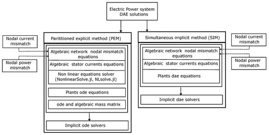
Figure 1.
Differential algebraic solution methods implemented in the package.
2.2.1. Dynamic Equations
The dynamics of synchronous machines can be represented as a combination of ODE equations and AE equations. A set of ODE equations describes the dynamics of the shaft (frequency and angular displacement), and dynamics of the stator fluxes. Two sets of algebraic equations define the relation between stator fluxes, stator current, field voltage, and rotor state variables. Various types of models for magnetic equations such as Sauer–Pai, Marconato, and Anderson–Fouad have been described in the literature. Simplified magnetic models of ODE equations, shaft dynamics ODE equations, and stator currents equations based on the one-d one-q axis are given in (8), (9), and (10), respectively:
2.2.2. Load Models
The representation of loads can take various forms, such as constant power, constant current, and constant impedance or a combination of each of the aforementioned load types. A generalised model of network load is given by (13):
where and represent constant active power and constant reactive power coefficients, respectively, and and denote the coefficients of active and reactive constant current magnitude at a constant power factor, while and represent the active and reactive coefficients of constant impedance. The three types of load models are available in the package.
2.2.3. Network Algebraic Equations
Network algebraic equations relate the nodal power balance or nodal current balance with network branches parameters, nodes voltages, and current injection at nodes and flow through branches. Network algebraic equations (power flow equations) can be represented in a power balance form or a current balance form. The representation of the power balance form for active and reactive power is given by (14) and (15). Similarly, the representation of the current balance form for real and imaginary node current is given by (16) and (17). The two types of representation are implemented in the package. The current balance representation is usually used in transient stability studies:
where , .
where , .
where , .
where , .
3. Description of ePowerSim Package and Subunits
ePowerSim.jl package is available for download at https://github.com/DSI-NRF-PENO/ePowerSim.jl (accessed on 19 September 2025) [30]. The design of the package is divided into eight subunits: (i) variables and parameters indexing; (ii) components parameters aggregation; (iii) models functions and variable symbols; (iv) callbacks generation; (v) results and visualisation; (vi) co-simulation interface; (vii) generic functions; and (viii) system initialisation.
3.1. ePowerSim Components Variables and Parameters Indexing
The indexing subunit is responsible for indexing components, state variables, algebraic variables, components parameters, and control variables. Data in various data format are first converted to json format as shown in Figure 2. The static components and dynamic components data are subsequently separated for the indexing of algebraic variables, components parameters, and state variables.
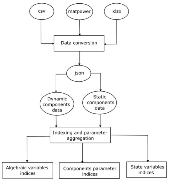
Figure 2.
Formulation of variables and parameters indices from input data.
3.2. Composition of Components, Variables and Functions in ePoweSim
Creation of a dynamic model of device requires, specification of its state variable symbols, components parameter symbols, state function, output function, init function, and in some cases a callback function. Illustration of codes listing for a generic excitation system are provided in Appendix A. The graphical formation of a dynamic model is shown in Figure 3. Similarly, Figure 4 depicts the formation of a model of a static device. A static device model only requires as inputs, algebraic variable symbols, component parameters symbols, and the algebraic equations that govern the behaviour of the device.
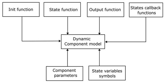
Figure 3.
Dynamic component model.
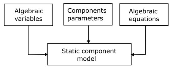
Figure 4.
Static component model.
The symbolic name of a component type and its state variable are first declared. This information is subsequently added to the appropriate lists in the component state symbols library. Dictionaries are created to hold init, dynamic, and output functions. The keys of the dictionaries are symbols of the component names.
Adding a new type of device requires creating an init function, dynamic function (state equations), output function and in some cases callback function. Once these functions are created, they should be added to the appropriate lists in the package.
3.3. Composition of Components Parameters Set in ePowerSim
The parameters aggregation subunit is responsible for extracting appropriate parameters from components that are used in specific models. The parameters are subsequently organised in data structures in conjunction with an indexing subunit. The creation of parameters for a model is shown in Figure 5.

Figure 5.
Parameter aggregation.
3.4. Composition of Callback Set in ePowerSim
Callbacks in Julia provide a reactive infrastructure for dynamic systems. These systems could be represented in different forms of dynamic equations, ordinary differential equations (ODEs), differential algebraic equations (DAEs), the Bounded Value Problem (BVP), stochastic differential algebraic equations (SDAEs), Delay Differential Equation (DDE), stochastic delay differential equation (SDDE), and stochastic differential equation (SDE) just to mention a few. Of interest to the modelling of power and energy systems and the optimisation of networks are differential algebraic equations (DAEs), stochastic differential algebraic equations (SDAEs), and the stochastic delay differential equation (SDDE). A dynamic model of electric power systems that incorporates the dynamics of generators, control devices, and network equations formulated in power flow formalism intrinsically takes the form of differential algebraic equations. Control of the states and algebraic variables of electric power systems necessitate the use of callbacks.
The callback unit in the package is based on the infrastructure of callbacks in DifferentialEquations.jl. Components that have states with callbacks can define the customised callbacks necessary for states. In addition, another set of callbacks can be added externally to the states event list and states affect list.
A typical event callback parameter requires the specification of an event function, the index of the state in which the event will occur in the system states indices, and the value of the state that constitutes an event. Similarly, affect callback parameters require the specification of the affect function, the index of the state that would be affected by the event in the system states indices, a function, or value of the state, post event. It should be noted that in the design of callback unit for the package, an event can affect the state it occurred in or another state. In addition, some events will require a change in the parameter values in addition to a change in state. Such events will require additional information on the set of parameters that would be changed.
3.5. System Initialisation
A snapshot of the processes involved in the system initialisation is shown in Figure 6 and Figure 7. A power flow set point is first calculated based on the operating parameter of a network. The results are then used for dynamic components initialisation as shown in Figure 6. The details of the dynamic components initialisation process are shown in Figure 7. The initialisation of a system starts with a call to the system init function. The system init function subsequently requests each dynamic device to initialise based on each device init function. In cases of components that have dynamic sub-components, the request is passed to sub-components to initialise based on each sub-component init function. The initialisation of each component and the sub-components initialisation state are aggregated by the system init unit for system initialisation.
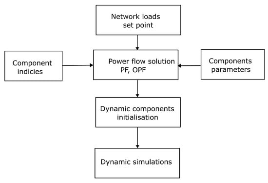
Figure 6.
Initial active power, reactive power, set points, and initialisation of state variables.
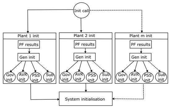
Figure 7.
Initialisation of state variables.
4. Models Validation
A validation process that was used to assess models of an electric power system in the package is presented in this section. The validation of models and output of simulations in the package were performed for both static and dynamic cases. The static performance validation was conducted by comparing the results of the ordinary power flow of IEEE 9 test systems obtained using the package with the result obtained from a real-time digital simulator for electric power systems (RTDS). The dynamic validation was conducted through a sudden increase in active power demand at a node in the IEEE 9 bus and IEEE 14 test systems. The results obtained from RTDS and the package were compared for validation purposes.
RSCAD is a graphical user interface software application that is used for management, configuration, and modelling in RTDS. It has two major interfaces for modelling (Draft) and control (Runtime). Components in the Runtime interface are directly linked to equivalent components in the Draft interface. RSCAD comes with a substantial number of benchmark test systems.
The runtime environment for the IEEE 9 bus and IEEE 16 bus test systems in RSCAD were modified to include a trigger unit to implement a sudden change in load at a bus. The trigger unit is shown in Figure 8. In general, the simulation time step in RTDS is 50 μs for the real-time simulation and integration of hardware-in-the-loop. Since the validation process is not meant to assess the real-time performance but the validity of the models, a few delays were introduced to ease simulation. The push button PB in Figure 8 triggers a close event of a circuit breaker in RSCAD Draft interface. When a push on PB is detected by an edge detect , the output of resets a timer (T). The output of the timer and trigger time serve as input to a comparator. Once the clock time exceeds the trigger time, a signal is sent to a circuit breaker to connect a load to a pre-determined bus. The load stays connected for the duration set in the edge detector with pulse duration . The pulse width of ED2 is set to . The simulation duration is determined by in combination with the output of timer T.
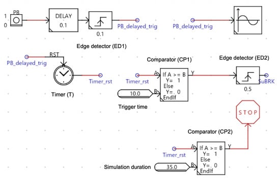
Figure 8.
RSCAD runtime trigger for sudden load change.
A sudden load change simulation in RTDS was conducted first; subsequently, the event time of the load change was determined to be . was then used as the event time for a sudden load change in ePowerSim.jl. The time step of output signals from ePowerSim.jl was set to in order to reduce the amount of output results without appreciably affecting the visualisation of the results. In addition, outputs from RTDS were down sampled to give of in order to align the results obtained in RTDS with the one obtained in ePowerSim.jl. The specification of the RTDS used for validation is provided in Table 1.

Table 1.
Specification of real-time digital simulator for electric power system used for validation.
4.1. Static Model Validation: IEEE 9 Bus Test System
The ordinary power flow results obtained from the package and RSCAD models are presented in Table 2 and Table 3. In addition, the results reported in [31] are also presented in the tables. It is evident from the tables that the results produced by the package for ordinary power flow is in agreement with RTDS and what was reported in [31]. Although the phase angle of the slack bus in RTDS result is −30.00°, this does not introduce any significant discrepancies since the relative phase angles of all buses voltages to the phase angle of the slack bus voltage is the same for the results obtained by the package.
Table 2.
Comparison of power flow results of the package with RTDS and PSS/E for the IEEE 9 bus test system.
Table 3.
Comparison of power flow results of ePowerSim.jl with RTDS and PSS/E voltage magnitude and angles at non-generation nodes for the IEEE 9 bus test system. Note that the ePowerSim.jl nodes numbering are based on MATPOWER data, with the following MATPOWER to RTDS node transformation , , , , .
4.2. Dynamic Model Validation: IEEE 9 Bus Test System
Similarly, dynamic model validation was conducted by a sudden increase and decrease in the active power demand at node 5 by within seconds as shown in Figure 9. The results obtained for the sudden perturbation of active power demand are presented in Figure 10a,b and Figure 11a,b. It can easily be seen that the result obtained from the package is in close agreement with the result obtained from RTDS.
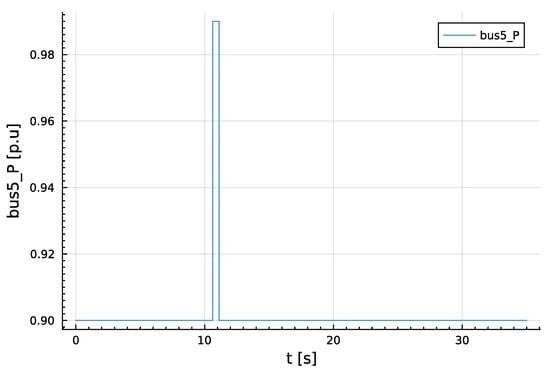
Figure 9.
Sudden load change at bus 5.
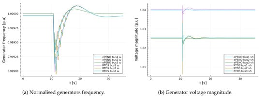
Figure 10.
Validation results for generators frequencies and voltage magnitudes for IEEE 9 bus test system model.
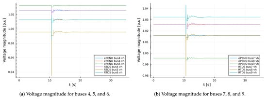
Figure 11.
Validation results for non-generators voltage magnitude for the IEEE 9 bus test system model.
4.3. Dynamic Model Validation: IEEE 14 Bus Test System
A dynamic model validation was also conducted by a sudden increase and decrease in the active power demand at node 10 by within seconds as shown in Figure 12a. The results obtained for the sudden perturbation of active power demand are presented in Figure 12, Figure 13 and Figure 14. An expanded view of change in frequency as a result of perturbation is shown in Figure 12b. It can easily be seen that the deviation in frequency during the steady state and system perpetuation are pu and pu. In addition, the result obtained from the package for voltage magnitude is in close agreement with the result obtained from RTDS, except for the voltage magnitude at bus 14. The difference in the values does not come from the dynamic characteristics of the model but the steady-state values (power flow). The values of the voltage magnitude at bus 14 based on ordinary power flow analysis for ePowerSim and RTDS are pu and pu, respectively.
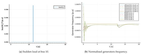
Figure 12.
Validation results for a sudden change in active power at bus 10 and generators frequencies for IEEE 14 bus test system model.
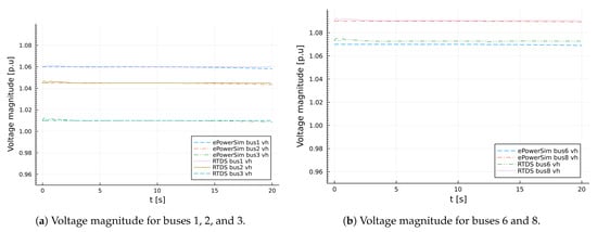
Figure 13.
Validation results for generators voltage magnitude for IEEE 14 bus test system model.
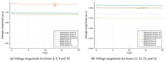
Figure 14.
Validation results for non-generators voltage magnitude for IEEE 14 bus test system model.
5. Use Cases of ePowerSim
The package is developed as a federation of functions for modelling, simulation, and analysis in electric power systems. Some of the modelling and simulation capabilities of the package are shown in Figure 15. In the following subsections, we present some of the use cases of the package, such as distributed slack power flow, optimal power flow, and dynamic load variation through co-simulation.
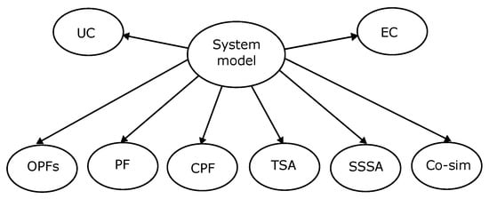
Figure 15.
Electric power system simulations and analysis schemes currently available in the package.
5.1. Distributed Slack
Distributed slack power flow entails the distribution of network losses among a set of generators in a network. Active power injections of generators in a distributed slack set are a combination of the nominal set-point power and a fraction of the total network loss based on the participation factor of individual generators in the set.
Network active power loss is given by (18)
where is the total network loss.
Active power injection by a generator in a distributed slack set is given by (19).
where and are a generator base power and generator loss participation factor, respectively.
Similarly, it is possible to designate a set of generators to pick up deviation in base load based on load deviation pick-up participation factor . The active power injection from a generator in load deviation pick-up set is given by (20)
where is the load deviation pick-up participation factor of a generator.
It is easy to show that the active power injection of a generator in set and is given by
A distributed slack power flow was conducted for the IEEE 14 bus test system. Generator 3, 6, and 8 are synchronous generators; consequently, only generators 1 and 2 are involved in slack distribution. Each of the two generators are allocated a weight of 0.5 each.
The slack value obtained by ePowerSim, PandaPower and [28] are pu, pu, and pu, respectively. Similarly, the reactive power loss result obtained by ePowerSim, PandaPower, and [28] are pu, pu, and pu, respectively. The results obtained for active power and reactive power generation by ePowerSim in comparison with PandaPower and ref. [28] are presented in Table 4. Similarly, the results for network buses voltage magnitude and angle are presented in Table 5. The value of active power generation pu obtained for generator 1 by ePowerSim is lower than the values obtained by PandaPower and [28] which are and , respectively. Conversely, the value of active power generation pu obtained for generator 2 by ePowerSim is higher than the values obtained by PandaPower and [28], which are and , respectively. Nevertheless, the values for reactive power generation obtained for all generators by ePowerSim is lower than the values obtained by PandaPower and [28].
Table 4.
Active power and reactive power generation of distributed slack power flow for IEEE 14 bus test system.
Table 5.
Network buses voltage magnitude and voltage phase angle for distributed slack power flow results for IEEE bus 14 test system.
5.2. Optimal Power Flow
A generic optimal power flow problem can be formulated as the minimisation of a cost function (objective function) in (22) subject to equality constraints in (23) and inequality constraints in (24)
and limits on the optimisation variables are .
The results obtained for optimal power flow by ePowerSim in comparison with PandaPower and the literature [28] are presented in Table 6 and Table 7. The objective values obtained by ePowerSim, PandaPower, and [28] are , , and , respectively.
Table 6.
Optimal power flow power generation for generation nodes.
Table 7.
Optimal power flow.
5.3. Dynamic Load Variation Through Co-Simulation
Co-simulation entails the simultaneous simulation of models of different entities with the coordination of data exchange between the entities through a broker. Helics.jl provides a framework for the co-simulation of models co-located on the same platform or different platforms. An instance of the simulation of a model on an entity is termed a federate. A simulation space of all federates and set of brokers that interact to exchange data is termed a federation. A federate may chose to publish data only (publication federate), subscribe to data only (subscriber federate), or publish and subscribe to some set of data (subscriber–publication federate). Figure 16 depicts federation for the co-simulation of five federates and a Helics broker. In Figure 16, fed 1 and fed k are publication federates; fed 2 is a subscriber federate; fed n and ePENO are publication–subscriber federates.
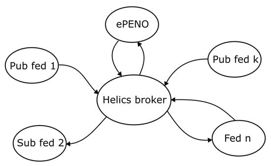
Figure 16.
A co-simulation federation.
Co-simulation of the dynamic model of the IEEE 14 bus test network (sdDynamicsHelicsSim), variable-phase, variable frequency oscillator (diffeqHelicsSim), a data recorder (dataReceiverHelicsSim), and a broker (Helics broker) is shown in Figure 17. diffeqHelicsSim is a publisher federate. It publishes one of its states . diffeqHelicsSim can represent any system or physical phenomenon that is external to an electric power system, but its states can affect the dynamics of an electric power system. It could be a weather pattern or any subject of interest. dataReceiverHelicsSim is a subscriber federate. It keeps a record of the events or data it subscribes to. In the co-simulation, it subscribes to four data from bus 4 of sdDynamicsHelicsSim federate; (i) voltage magnitude , (ii) voltage phase angle , (iii) active power , and (iv) reactive power . sdDynamicsHelicsSim is a publisher and subscriber federate. It subscribes to angular deviation from diffeqHelicsSim. The value of is used to modify the active power at bus 4 in the electric system. It also publishes the voltage magnitude , voltage phase angle , active power , and reactive power at bus 4.
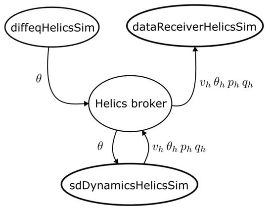
Figure 17.
ePowerSim model co-simulation with independent federates.
The settings with regards to the co-simulation environment are (i) data exchange protocol , (ii) the time difference between data sample instances , (iii) offset time , and (iv) polling (period) time ,
The dynamic model of diffeqHelicsSim is a simple pendulum with an external forcing function given by (25)
where and are the angular frequency and angular deviation, respectively. , , and are the length of the pendulum, acceleration due to gravity, and mass of the pendulum, respectively.
Figure 18a depicts the states of diffeqHelicsSim federate, while Figure 18b depicts the published data from diffeqHelicsSim federate and the subscription data by sdDynamicsHelicsSim. It is evident from Figure 18b that there is no difference between the value of what is published by diffeqHelicsSim and what is received by sdDynamicsHelicsSim.
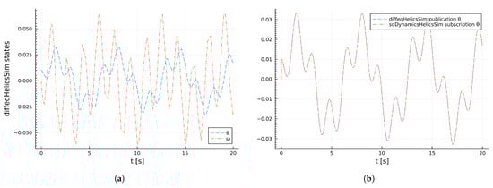
Figure 18.
Fedrates publications and subscriptions. (a) diffeqHelicsSim (Oscilator) states. (b) diffeqHelicsSim publication and sdDynamicsHelicsSim subscription.
Similarly, Figure 19a depicts the data published by sdDynamicsHelicsSim federate: voltage magnitude , voltage phase angle , active power , and reactive power . Figure 19a,b are presented separately, in order to not obscure their details. It can easily be seen in the two figures that there is no difference between the data published by sdDynamicsHelicsSim and the subscription by DataReceiverHelicsSim.
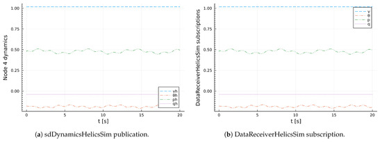
Figure 19.
DataReceiverHelicsSim subscriptions and sdDynamicsHelicsSim publications.
The effect of the state of the diffeqHelicsSim federate on the dynamics of sdDynamicsHelicsSim federates is presented in Figure 20 and Figure 21. Figure 20a,b depict the voltage magnitude and voltage angle at generator buses, respectively. It can easily be seen in the two figures that the impact of variation in the state of diffeqHelicsSim on the generator buses voltage magnitude is not significant, compared to generator bus phase angles. In general, voltages at the generator buses are held relatively constant by automatic voltage regulators; hence, the variation in voltage magnitudes is not substantial.
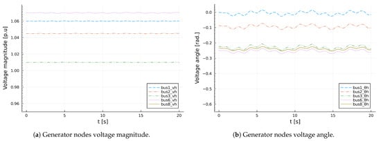
Figure 20.
Generator nodes voltage magnitude and generators voltage angle.
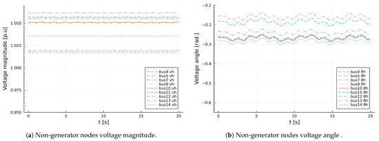
Figure 21.
Non-generator nodes voltage magnitude and Generators voltage angle.
The plot of voltage magnitude and voltage angle for non-generator buses are presented in Figure 21a and Figure 21b respectively. Similar to the observation with regards to generator buses, the variations in voltage magnitude is relatively low compared to the variations voltage phase angle at non-generator buses. Nevertheless, it is generally higher compared to variations in voltage magnitude at generator buses.
6. Conclusions
In this work, ePowerSim.jl, an open-source package in Julia programming language with co-simulation capability, is introduced for electric power system modelling, simulation, and analysis. The package provides a framework for research experimentation and pedagogical engagement. It conceptually factors electric power system model into two independent units: uniform parameter and index interface; and simulation and analysis-specific algorithms. This enables decoupling the modelling of electric power system components and operational entities from algorithms for specific simulation types. It also ensures that solvers for numerical computation can easily be swapped.
The essential features of ePowerSim presented in this paper are as follows:
- A close match between the results obtained in the simulation of an electric power system static and dynamic models in ePowerSim.jl and a real-time digital simulator during validation indicates that the package can be used for experimentation where there is no need for hardware-in-the-loop.
- ePowerSim produces comparatively good results for distributed slack power flow and optimal power flow. The package provides a common interface for the modelling, simulation, and analysis of static and dynamic behaviour of electric power systems.
- ePowerSim provides a framework for the co-simulation of electric power system models with external dynamic systems and events. This implies that an investigation of the impact of an external dynamic system can be conducted with ePowerSim.
The package already has models of synchronous machines, synchronous condensers, governors, power system stabiliser, automatic voltage regulators, and exciters. Nevertheless, in the future, models of inverters, asynchronous machines, rectifier models and energy storage systems would be added to the package.
Author Contributions
Conceptualisation, A.Y.; methodology, A.Y.; software, A.Y.; validation, A.Y. and T.M.; formal analysis, A.Y.; writing—original draft preparation, A.Y.; writing—review and editing, T.M.; visualisation, T.M.; project administration, T.M.; funding acquisition, A.Y. All authors have read and agreed to the published version of the manuscript.
Funding
This research was funded by Department Science Innovation-National Research Foundation South Africa (DSI-NRF) grant number 150573.
Data Availability Statement
The data used in this paper and ePowerSim.jl package are available at https://github.com/DSI-NRF-PENO/ePowerSim.jl (accessed on 19 September 2025).
Conflicts of Interest
The authors declare no conflicts of interest. The funders had no role in the design of the study; in the collection, analyses, or interpretation of data; in the writing of the manuscript; or in the decision to publish the results.
Abbreviations
The following abbreviations are used in this manuscript:
| AE | Algebraic equations |
| AVR | Automatic voltage regulator |
| CPF | Continuation power flow |
| Co-Sim | Co-simulation |
| DAE | Differential-algebraic equations |
| ED | Economic dispatch |
| GUI | Graphic user interface |
| ODE | Ordinary differential equations |
| OPF | Optimal power flow |
| PF | Ordinary power flow |
| RTDS | Real-Time digital simulator |
| SDAE | Stochastic differential algebraic equations |
| SDDAE | Stochastic delay differential algebraic equations |
| SSSA | Small-signal stability analysis |
| TSA | Transient stability analysis |
| UC | Unit commitment |
Appendix A
| Listing A1. Excitation system init function. |
 |
| Listing A2. Excitation system output function. |
 |
| Listing A3. Excitation system state function. |
 |
 |
| Listing A4. Excitation system callback function. |
 |
 |
References
- Rehtanz, C.; Guillaud, X. Real-time and co-simulations for the development of power system monitoring, control and protection. In Proceedings of the 2016 Power Systems Computation Conference (PSCC), Genoa, Italy, 20–24 June 2016; pp. 1–20. [Google Scholar] [CrossRef]
- Suvorov, A.; Gusev, A.; Ruban, N.; Andreev, M.; Askarov, A.; Ufa, R.; Razzhivin, I.; Kievets, A.; Bay, J. Potential Application of HRTSim for Comprehensive Simulation of Large-Scale Power Systems with Distributed Generation. Int. J. Emerg. Electr. Power Syst. 2019, 20, 20190075. [Google Scholar] [CrossRef]
- Gagnon, R.; Turmel, G.; Larose, C.; Brochu, J.; Sybille, G.; Fecteau, M. Large-scale real-time simulation of wind power plants into Hydro-Québec power system. In Proceedings of the 9th International Workshop on Large-Scale Integration of Wind Power into Power Systems as Well as on Transmission Networks for Offshore Wind Power Plants, Hydro, QC, Canada, 18–19 October 2010; pp. 18–19. [Google Scholar]
- Bam, L.; Jewell, W. Review: Power system analysis software tools. In Proceedings of the IEEE Power Engineering Society General Meeting, San Francisco, CA, USA, 16 June 2005; Volume 1, pp. 139–144. [Google Scholar] [CrossRef]
- Milano, F. An open source power system analysis toolbox. IEEE Trans. Power Syst. 2005, 20, 1199–1206. [Google Scholar] [CrossRef]
- Top, P.; Woodward, C.; Smith, S.; Banks, L.; Kelley, B. Dynamic Power Grid Simulation; Technical Report; Lawrence Livermore National Laboratory (LLNL): Livermore, CA, USA, 2015.
- Zimmerman, R.D.; Murillo-Sánchez, C.E.; Thomas, R.J. MATPOWER: Steady-State Operations, Planning, and Analysis Tools for Power Systems Research and Education. IEEE Trans. Power Syst. 2011, 26, 12–19. [Google Scholar] [CrossRef]
- Thurner, L.; Scheidler, A.; Schäfer, F.; Menke, J.H.; Dollichon, J.; Meier, F.; Meinecke, S.; Braun, M. Pandapower—An Open-Source Python Tool for Convenient Modeling, Analysis, and Optimization of Electric Power Systems. IEEE Trans. Power Syst. 2018, 33, 6510–6521. [Google Scholar] [CrossRef]
- Brown, T.; Hörsch, J.; Schlachtberger, D. PyPSA: Python for Power System Analysis. J. Open Res. Softw. 2018, 6, 4. [Google Scholar] [CrossRef]
- Cui, H.; Li, F. ANDES: A Python-Based Cyber-Physical Power System Simulation Tool. In Proceedings of the 2018 North American Power Symposium (NAPS), Fargo, ND, USA, 9–11 September 2018; pp. 1–6. [Google Scholar] [CrossRef]
- Cui, H.; Li, F.; Tomsovic, K. Hybrid Symbolic-Numeric Framework for Power System Modeling and Analysis. IEEE Trans. Power Syst. 2021, 36, 1373–1384. [Google Scholar] [CrossRef]
- Bezanson, J.; Karpinski, S.; Shah, V.B.; Edelman, A. Julia: A fast dynamic language for technical computing. arXiv 2012, arXiv:1209.5145. [Google Scholar] [CrossRef]
- Bezanson, J.; Edelman, A.; Karpinski, S.; Shah, V.B. Julia: A fresh approach to numerical computing. SIAM Rev. 2017, 59, 65–98. [Google Scholar] [CrossRef]
- Coffrin, C.; Bent, R.; Sundar, K.; Ng, Y.; Lubin, M. PowerModels.JL: An Open-Source Framework for Exploring Power Flow Formulations. In Proceedings of the 2018 Power Systems Computation Conference (PSCC), Dublin, Ireland, 11–15 June 2018; pp. 1–8. [Google Scholar] [CrossRef]
- Lara, J.D.; Barrows, C.; Thom, D.; Krishnamurthy, D.; Callaway, D. PowerSystems.jl—A power system data management package for large scale modeling. SoftwareX 2021, 15, 100747. [Google Scholar] [CrossRef]
- Lara, J.D.; Barrows, C.; Thom, D.; Dalvi, S.; Callaway, D.S.; Krishnamurthy, D. PowerSimulations.jl—A Power Systems operations simulation Library. arXiv 2024, arXiv:2404.03074. [Google Scholar]
- Plietzsch, A.; Kogler, R.; Auer, S.; Merino, J.; Gil-de Muro, A.; Liße, J.; Vogel, C.; Hellmann, F. PowerDynamics.jl—An experimentally validated open-source package for the dynamical analysis of power grids. SoftwareX 2022, 17, 100861. [Google Scholar] [CrossRef]
- Philpott, T.; Agalgaonkar, A.P.; Brinsmead, T.; Muttaqi, K.M. An Open-Source Julia Package for RMS Time-Domain Simulations of Power Systems. Energies 2024, 17, 5677. [Google Scholar] [CrossRef]
- Lara, J.D.; Barrows, C.; Thom, D.; Dalvi, S.; Callaway, D.S.; Krishnamurthy, D. PowerSimulationsDynamics.jl—An Open Source Modeling Package for Modern Power Systems with Inverter-Based Resources. arXiv 2024, arXiv:2308.02921. [Google Scholar]
- Rackauckas, C.; Nie, Q. DifferentialEquations.jl—A performant and feature-rich ecosystem for solving differential equations in Julia. J. Open Res. Softw. 2017, 5, 15. [Google Scholar] [CrossRef]
- Rackauckas, C.; Innes, M.; Ma, Y.; Bettencourt, J.; White, L.; Dixit, V. Diffeqflux.jl—A julia library for neural differential equations. arXiv 2019, arXiv:1902.02376. [Google Scholar]
- Hindmarsh, A.C.; Brown, P.N.; Grant, K.E.; Lee, S.L.; Serban, R.; Shumaker, D.E.; Woodward, C.S. SUNDIALS: Suite of nonlinear and differential/algebraic equation solvers. ACM Trans. Math. Softw. (TOMS) 2005, 31, 363–396. [Google Scholar] [CrossRef]
- Gardner, D.J.; Reynolds, D.R.; Woodward, C.S.; Balos, C.J. Enabling new flexibility in the SUNDIALS suite of nonlinear and differential/algebraic equation solvers. ACM Trans. Math. Softw. (TOMS) 2022, 48, 31. [Google Scholar] [CrossRef]
- Veltz, R. BifurcationKit.jl. 2020. Available online: https://hal.archives-ouvertes.fr/hal-02902346 (accessed on 19 September 2025).
- Lubin, M.; Dowson, O.; Garcia, J.D.; Huchette, J.; Legat, B.; Vielma, J.P. JuMP 1.0: Recent improvements to a modeling language for mathematical optimization. Math. Program. Comput. 2023, 15, 581–589. [Google Scholar] [CrossRef]
- Hardy, T.D.; Palmintier, B.; Top, P.L.; Krishnamurthy, D.; Fuller, J.C. HELICS: A co-simulation framework for scalable multi-domain modeling and analysis. IEEE Access 2024, 12, 24325–24347. [Google Scholar] [CrossRef]
- Sauer, P.W.; Pai, M. Power System Dynamics and Stability; Prentice Hall: Hoboken, NJ, USA, 1997. [Google Scholar]
- Milano, F. Power System Modelling and Scripting; Springer Science & Business Media: Berlin/Heidelberg, Germany, 2010. [Google Scholar]
- Pal, A.; Holtorf, F.; Larsson, A.; Loman, T.; Schaefer, F.; Qu, Q.; Edelman, A.; Rackauckas, C. NonlinearSolve. jl: High-Performance and Robust Solvers for Systems of Nonlinear Equations in Julia. arXiv 2024, arXiv:2403.16341. [Google Scholar]
- Yusuff, A.A. ePowerSim.jl: A Framework for Modelling, Simulation and Analysis of Energy and Power Systems. 2025. Available online: https://github.com/DSI-NRF-PENO/ePowerSim.jl (accessed on 19 September 2025).
- RSCAD FX, version 2.3; IIIRTDS Technologies: Winnipeg, MB, Canada, 2024.
Disclaimer/Publisher’s Note: The statements, opinions and data contained in all publications are solely those of the individual author(s) and contributor(s) and not of MDPI and/or the editor(s). MDPI and/or the editor(s) disclaim responsibility for any injury to people or property resulting from any ideas, methods, instructions or products referred to in the content. |
© 2025 by the authors. Licensee MDPI, Basel, Switzerland. This article is an open access article distributed under the terms and conditions of the Creative Commons Attribution (CC BY) license (https://creativecommons.org/licenses/by/4.0/).