Assessing Time Series Foundation Models for Probabilistic Electricity Price Forecasting: Toward a Unified Benchmark

Abstract

Probabilistic electricity price forecasting (PEPF) is a highly complex task with broad economic and operational impact. Recent advances in time series foundation models (TSFMs) offer promising tools to improve PEPF performance. In contrast, PEPF provides a challenging platform for evaluating and accelerating the development of general TSFMs. Despite their potential synergies, TSFMs have received limited attention in the PEPF literature, while the PEPF task remains largely unexplored in the TSFM context. This work aims to bridge these currently parallel research streams, fostering convergence and cross-fertilization to advance both fields. Focusing on Moirai, an open-source probabilistic framework with native covariate support and fine-tuning capabilities, we set up a comprehensive benchmark against specialized neural network-based PEPF methods across multiple market regions characterized by high variability and heterogeneous conditions. Additionally, we systematically explore fine-tuning strategies and model configurations, including context lengths and exogenous variable usage, to assess their impact on probabilistic forecasting accuracy. Experimental results indicate that Moirai provides promising zero-shot predictions, though it still underperforms compared to domain-specific neural networks. Fine-tuning improves calibration, while the architecture does not yet fully leverage exogenous features. Taken together, these observations offer valuable insights to foster future developments. We release our code through an open repository to facilitate collaborative progress within the PEPF and TSFM communities.

1. Introduction

Electricity price forecasting (EPF) is an inherently complex task whose difficulty continues to grow alongside the evolving dynamics of modern power markets [1,2]. As a nonstorable commodity, electricity exhibits price behaviors influenced by multiple factors, including weather conditions, weekdays, and peak versus off-peak hours [3]. Furthermore, the increasing penetration of renewable energy sources [4], combined with the impact of geopolitical events [5], has become a fundamental driver of day-ahead price variability, introducing additional uncertainty into market behavior.

Early research in EPF has primarily focused on point forecasting, predominantly leveraging statistical models such as ARIMA and ETS [6]. More recently, considerable attention has been devoted to deep learning methods, driven by the growing availability of computational power, advanced tools, and large-scale datasets [7].

The significant inherent volatility of electricity markets demands forecasting methods that are not only accurate but also capable of providing reliable uncertainty quantification. Such probabilistic forecasts are essential for robust and informed decision making in power systems [8]. Consequently, probabilistic electricity price forecasting (PEPF) has gained considerable traction, becoming a central focus of current research [9,10]. Improved performance in PEPF directly translates into tangible economic and operational benefits for various stakeholders. Utilities, retailers, aggregators, and large consumers rely on PEPF outputs to optimize trading strategies, schedule resources efficiently, and make optimal commitment decisions under uncertainty by accounting for associated risks [11,12].

Among the various probabilistic forecasting methodologies, neural-network-based models have attracted substantial attention due to their inherent flexibility in extracting latent representations and modeling intricate dependencies embedded within the high-dimensional input conditioning space [8]. In particular, distributional deep neural networks (D-DNNs) and quantile-regression-based techniques have demonstrated strong potential for accurately modeling the complex conditional patterns of electricity price distributions [13,14]. A wide range of architectural forms has been explored for this purpose (see, e.g., [15]). Nevertheless, deep feed-forward networks remain a benchmark that is challenging to outperform [16]. These models are typically classified as local approaches, aimed at effectively capturing dataset-specific features. In contrast, global models are designed to extract shared features from collections of time series, enabling them to generalize across multiple datasets and support forecasting on previously unseen data. Such models leverage the representational capacity of advanced deep learning architectures—including transformers [17]—to capture cross-series dependencies. Notable examples include DeepAR [18], N-BEATS [19], and TiDE [20]. Despite their success in various forecasting domains, the application of global models to electricity price forecasting remains limited. Reference [8] performed an empirical assessment of several global architectures, including DeepAR, DeepTCN, DSANet, and LSTNet. Reference [21] developed the NBEATSx model to enhance interpretability. A global PEPF model trained on multiple day-ahead power markets have been proposed in [22], leveraging a spatio-temporal architecture incorporating graph-based market topology information. Still, the development of generic models that operate under real-world constraints faces critical challenges, including the need to capture market-specific dynamics, comply with diverse regulatory frameworks, and manage heterogeneous data sources. These issues become even more pronounced in rapidly evolving energy systems, such as those undergoing major reforms (e.g., China’s electricity market) [23].

Motivated by the success of large pretrained models in natural language processing (NLP), particularly transformer-based architectures, recent research has begun exploring analogous paradigms for general time series forecasting. First approaches include PromptCast [24], which reformulates time series data as text prompts for existing large language models (LLMs), and LLMTime [25], which represents numerical data as tokenized digit strings for models such as GPT-3 or LLaMA-2, thus demonstrating the feasibility of zero-shot forecasting. Additional efforts, such as GPT4TS [26] and Time-LLM [27], adapt large pretrained LLMs for time series applications through architectural modifications. Nevertheless, the required dataset-specific fine-tuning constitutes a significant barrier that limits broader applicability and generalizability.

To address these challenges, recent research has focused on developing time series foundation models (TSFMs) inherently trained on temporal data. TSFMs are designed to leverage pretrained representations that capture a wide range of temporal patterns and contextual dependencies, enabling accurate forecasting across diverse domains without (or minimal) task-specific fine-tuning requirements. The emergence of large-scale temporal datasets—such as LOTSA [28], Chronos-datasets [29], and GIFT-Eval [30]—has been instrumental in enabling this paradigm shift. Consequently, the family of TSFMs is rapidly expanding and has already demonstrated competitive zero-shot performance on multiple open benchmarks [30,31].

Despite significant advances in the broader machine learning community, the potential of foundation models to address emerging challenges in PEPF remains largely underexplored. Given the intrinsic complexity and volatility of electricity markets [32], PEPF represents a particularly demanding real-world application—beyond those previously studied with time series foundation models—that provides a valuable context to evaluate model performance, identify existing limitations, and explore avenues for future development.

Contributions and Organization of the Paper

Building upon seminal prior works, the primary contribution of this study is to advance the understanding of TSFMs’ potential in addressing challenging tasks such as probabilistic electricity price forecasting (PEPF) in day-ahead markets, an area traditionally dominated by specialized models and neural network architectures. Specifically, we focus on the Moirai foundation models [28], a general-purpose TSFM offering an open-source probabilistic framework with support for covariates and fine-tuning. This enables coherent and reproducible comparisons with state-of-the-art PEPF approaches based on local distributional neural networks. To this end, we establish a rigorous benchmark leveraging the growing open data source provided by the ENTSO-E transparency platform [33], and adopt an experimental protocol aligned with best practices in the PEPF domain (see, e.g., [16]). First, we assess Moirai’s zero-shot performance against specialized forecasting techniques across multiple European markets under realistic, high-variability conditions. Next, we systematically explore the TSFM configuration space—varying context lengths, stationary conditions, and the inclusion of exogenous variables—to derive actionable insights into adapting general-purpose models to domain-specific challenges. Finally, we propose PEPF as a valuable testbed for TSFM development due to its economic relevance and modeling complexity, and release our full experimental framework in a public repository (link: https://github.com/MarchesiGabriele/PEPF_bench, release v1.0, 27 October 2025) to foster reproducibility and collaborative progress within both communities.

The rest of this paper is organized as follows. Section 2 introduces the probabilistic electricity price forecasting problem, followed by a description of the specialized distributional neural network models used as baselines for comparison. The section also reviews relevant foundation models proposed in the literature and discusses the rationale for selecting the Moirai architecture as the first TSFM candidate in our experimental framework. Subsequent sections deepen the deployed PEPF benchmarks and the explored model configurations, as well as the evaluation metrics deployed in the analysis. Then, Section 3 reports and discusses the experimental findings. Finally, Section 5 concludes the paper and outlines potential avenues for future research.

2. Materials and Methods

2.1. Specialized Distributional Deep Neural Networks for PEPF

Probabilistic electricity price forecasting (PEPF) is a specialized task within the broader domain of probabilistic time series forecasting. Its primary objective is to predict future electricity prices while reliably quantifying the associated uncertainty. This uncertainty can be represented at different levels of detail, ranging from distributional summaries (e.g., quantiles or prediction intervals) to full predictive distributions. In this work, we focus on the latter, providing a comprehensive characterization of the predictive distribution.

Given historical observations and relevant exogenous variables (such as power demand, renewable generation, and fuel prices), the goal is to estimate the conditional distribution of future prices $p(y_{t+1},\dots ,y_{t+h}\mid {\mathcal{X}}_t)$ across forecast horizons $h=1,\dots ,H$, where ${\mathcal{X}}_t$ denotes the information set available at time t. From distributional forecasts, key probabilistic summaries can be derived, including prediction intervals and quantiles, as well as scenario trajectories, which are essential for risk-aware decision making in electricity markets.

In recent years, neural networks have emerged as powerful tools for this purpose, offering the flexibility to capture complex nonlinear dependencies and temporal patterns. These are commonly referred to as distributional deep neural networks (D-DNNs) in the PEPF context. Formally, this can be expressed as the functional mapping:

$$\widehat{p}(y_{t+1},\dots ,y_{t+h}\mid {\mathcal{X}}_t)=f_{\mathsf{\Theta }}\left({\mathcal{X}}_t\right),$$

(1)

where $f_{\mathsf{\Theta }}$ is a neural network parameterized by $\mathsf{\Theta }$, and $\widehat{p}(·)$ denotes the predicted approximate conditional distribution of future prices $y_{t+1},\dots ,y_{t+h}$. The input ${\mathcal{X}}_t$ encodes both historical prices and exogenous features (see, e.g., [14]).

Hence, D-DNNs extend classical neural-network-based point prediction in EPF by introducing an output layer providing the parameters of the conditional distribution. In this study, we adopt the architecture of the state-of-the-art D-DNN proposed by [13] for PEPF, which is based on feed-forward mappings. Exploration of alternative architectural designs, such as transformer-based models or hybrid ensembles, is deferred to future work. Considering two hidden layers with $n_{h_1},n_{h_2}\in {\mathbb{Z}}^{+}$ units to lighten notation, this is mathematically expressed as follows:

$$\begin{array}{cc}\hfill {\ell }_1& =g({\mathcal{X}}_t{W}_1+b_1),\hfill \\ \hfill {\ell }_2& =g({\ell }_1{W}_2+b_2)W_3+b_3,\hfill \end{array}$$

(2)

where $W_1\in {\mathbb{R}}^{n_i\times n_{h_1}}$, $W_2\in {\mathbb{R}}^{n_{h_1}\times n_{h_2}}$, $W_3\in {\mathbb{R}}^{n_{h_2}\times n_p}$, and $b_1\in {\mathbb{R}}^{n_{h_1}}$, $b_2\in {\mathbb{R}}^{n_{h_2}}$, $b_3\in {\mathbb{R}}^{n_p}$ represent the weight and bias parameters. Here, $g(·)$ is a nonlinear activation function (e.g., ReLU), and $n_p\in {\mathbb{Z}}^{+}$ denotes the number of distribution parameters.

Several output density forms have been explored in the literature (see, e.g., [14] and references therein). In this study, we focus on the flexible Johnson’s SU (JSU) distribution to implement the specialized PEPF baseline. This choice is primarily driven by its widespread adoption in recent deep distributional neural network studies for PEPF, where JSU has become a de facto standard due to its enhanced flexibility and competitive performance. Alternative parameterizations, such as the standard normal, have also been considered in prior work; however, JSU offers a richer characterization of location, scale, skewness, and tailweight, which are crucial for capturing the heavy tails and asymmetry often occurring in electricity price time series. While this study focuses on JSU, the exploration of alternative output distributions is left to future work.

Formally, the Johnson’s SU probability density function is defined for each step in the forecasting horizon $h=1,\dots ,H$ as follows:

$$f^h\left(\chi \right)={\displaystyle \frac{{\xi }_t^h}{{\sigma }_t^h\sqrt{2\pi }}}{\displaystyle \frac{1}{\sqrt{1+{\left(\frac{\chi -{\mu }_t^h}{{\sigma }_t^h}\right)}^2}}}\exp \left[-{\displaystyle \frac{1}{2}}{\left({\zeta }_t^h+{\xi }_t^h{\sinh }^{-1}\left({\displaystyle \frac{\chi -{\mu }_t^h}{{\sigma }_t^h}}\right)\right)}^2\right],$$

(3)

where the parameters are obtained from the last hidden layer ${\ell }_2$ as

$$\begin{array}{cc}\hfill {\mu }_t^h& ={\ell }_2^{\left[h\right]},\hfill \end{array}$$

(4)

$$\begin{array}{cc}\hfill {\sigma }_t^h& =ϵ+\gamma \mathrm{Softplus}\left({\ell }_2^{[H+h]}\right),\hfill \end{array}$$

(5)

$$\begin{array}{cc}\hfill {\xi }_t^h& =1+\gamma \mathrm{Softplus}\left({\ell }_2^{[2H+h]}\right),\hfill \end{array}$$

(6)

$$\begin{array}{cc}\hfill {\zeta }_t^h& ={\ell }_2^{[3H+h]},\hfill \end{array}$$

(7)

$$\begin{array}{cc}\hfill \mathrm{Softplus}\left(x\right)& =\log (1+e^x),\hfill \end{array}$$

(8)

with $ϵ,\gamma >0$ as small positive constants for numerical stability and scaling. Here, ${\mu }_t^h$, ${\sigma }_t^h$, ${\xi }_t^h$, and ${\zeta }_t^h$ represent location, scale, tailweight, and skewness parameters of the Johnson’s SU distribution, respectively. The overall network is trained end-to-end by minimizing the negative log-likelihood over datasets constructed from available observations using moving windows with a fixed-length context. Within the distributional learning framework, the model outputs the parameters of the Johnson’s SU distribution conditioned on the input features. These parameters are generated by a dedicated distributional output layer, which is directly fed by the final hidden layer of the backbone neural network. The entire architecture, including both the feature extraction and distributional components, is jointly optimized via gradient-based training. Typically, D-DNNs are developed in a dataset-specific fashion (e.g., separately for each regional market), representing instances of local models.

2.2. Investigated Time Series Foundation Model

As introduced in Section 1, recent years have witnessed the emergence of numerous foundation models for time series forecasting, featuring novel architectural innovations, pretraining methodologies, and benchmark datasets. Lag-Llama [34], among the earliest proposed architectures, has paved the way for significant developments in the TSFM field. Subsequently, several models have emerged, demonstrating superior empirical performance. Chronos [29], based on the T5 encoder–decoder architecture [35], employs token quantization to discretize time series into a fixed vocabulary. TimesFM [36] adopts a decoder-only architecture that segments series into patches and leverages patch masking to enhance training efficiency. Moirai [28] utilizes a masked encoder design, enabling the joint processing of multivariate series by flattening the data. Toto [37] is a decoder-only model augmented with specialized modules to improve representation of multivariate observability. Other notable contributions include TTM [38], TabPFN-ts [39], MOMENT [40], and TimeGPT [41].

To establish the initial version of the benchmark, we selected the Moirai TSFM. Beyond its competitive performance on open benchmarks, this choice was motivated by the need to create a consistent experimental setup aligned with the D-DNN framework, thereby enabling fair and coherent comparisons. Moirai’s inherent support for covariates, fine-tuning capabilities, and availability within an open-source probabilistic framework rendered it particularly suitable. These features, summarized in Table 1, justify the preference for Moirai (marked in Green color) over alternative solutions available at the time of our experimental setup development. It is important to note that this study focuses on a general-purpose TSFM (i.e., not specifically trained on PEPF data), with the exploration of global and foundation models tailored for PEPF tasks left to future research. As introduced in Section 1, the objective of this work is not to conduct an exhaustive analysis of all recent TSFM innovations—interested readers are referred to the recent survey by [42]—but, rather, to establish a first common benchmark with potential for future extension. Given the rapid evolution of the TSFM literature, our study constitutes an initial step toward exploring the broad spectrum of TSFM developments. To this end, our experimental framework—provided as an open-source repository—is designed to facilitate the investigation of future models and advancements.

Table 1. Comparison of foundation models with different capabilities. ✓: supported, ✗: not supported.

Model	Probabilistic	Native Covariates Support	Finetune Support	Open-Source
ttm	✗	✓	✓	✓
tabpfn-ts	✓	✓	✗	✓
timesfm	✓	✗	✓	✓
chronos	✓	✗	✓	✓
moment	✗	✓	✓	✓
toto	✓	✓	✗	✓
timegpt	✓	✓	✓	✗
moirai	✓	✓	✓	✓

The Moirai architecture is briefly summarized in the following section to outline its principal features, thereby rendering the discussion self-contained. For comprehensive details, the reader is referred to the original publication [28].

2.2.1. Deployed Moirai Architectures

Moirai is built as a masked-encoder transformer specifically designed for time series forecasting across diverse frequencies, covariate structures, and data distributions. All covariates are concatenated into a single input sequence, subsequently partitioned into nonoverlapping patches and projected into a vector representation. The model accommodates variable patch dimensions, allowing flexible adaptation to time series with differing temporal resolutions. The masking mechanism employs learnable embeddings that span the forecast horizon, effectively covering the corresponding patches.

The model produces output tokens that parameterize a mixture distribution with c components, whose probability density function is expressed as follows:

$$p(y_{t+1},\dots ,y_{t+h}|\widehat{\mathsf{\Phi }})=\sum _{i=1}^c{w}_i{p}_i(y_{t+1},\dots ,y_{t+h}|{\widehat{\mathsf{\Phi }}}_i),$$

(9)

where $\widehat{\mathsf{\Phi }}=\{w_1,{\widehat{\mathsf{\Phi }}}_1,\dots ,w_c,{\widehat{\mathsf{\Phi }}}_c\}$, and $p_i$ denotes the probability density function of the i-th component.

Each component $p_i$ corresponds to a distinct probability distribution designed to capture different statistical behaviors observed in time series data. Specifically, Moirai employs a mixture of the following four distributions:

Student’s t-Distribution

$$p(x;\nu ,\mu ,\tau )={\displaystyle \frac{\mathsf{\Gamma }\left(\frac{\nu +1}{2}\right)}{\mathsf{\Gamma }\left(\frac{\nu }{2}\right)\sqrt{\pi \nu }\tau }}{\left(1+{\displaystyle \frac{1}{\nu }}{\left({\displaystyle \frac{x-\mu }{\tau }}\right)}^2\right)}^{-{\displaystyle \frac{\nu +1}{2}}},$$

(10)

with parameters $\nu >0$, $\mu \in \mathbb{R}$, and $\tau >0$ corresponding to the degrees-of-freedom, location, and scale, respectively. $\mathsf{\Gamma }(·)$ denotes the gamma function.

Log-Normal Distribution

$$p(x;\mu ,\sigma )={\displaystyle \frac{1}{x\sigma \sqrt{2\pi }}}\exp \left[-{\displaystyle \frac{{(\ln x-\mu )}^2}{2{\sigma }^2}}\right],$$

(11)

where $\mu \in \mathbb{R}$ and $\sigma >0$.

Negative Binomial Distribution

$$p(x;r,p)\propto {\displaystyle \frac{\mathsf{\Gamma }(x+r)}{\mathsf{\Gamma }(x+1)\mathsf{\Gamma }\left(r\right)}}{(1-p)}^x{p}^r,$$

(12)

given parameters $r>0$ and $p\in [0,1]$, with $\mathsf{\Gamma }(·)$ again denoting the gamma function.

Low-Variance Normal Distribution

$$p(x;\mu ,\sigma )={\displaystyle \frac{1}{\sigma \sqrt{2\pi }}}\exp \left[-{\displaystyle \frac{{(x-\mu )}^2}{2{\sigma }^2}}\right],$$

(13)

where $\mu \in \mathbb{R}$ and $\sigma >0$. For consistency, all distribution equations are presented in accordance with the formulation introduced in the Moirai paper [28].

The model was pretrained on the LOTSA dataset, which contains over 27 billion observations from time series spanning multiple domains, frequencies, and covariate configurations. Notably, no electricity price data were included during pretraining, making it suitable for zero-shot forecasting evaluation in our study. We employ the publicly available moirai-1.1-R model (at the time of writing, this represents the most recent Moirai release supporting distributional forecasting. Moirai2 has been excluded, as it produces only quantile forecasts (from 0.1 to 0.9); however, it remains under consideration for future investigation) in its small, base, and large configurations, comprising 13.8 M, 91.4 M, and 311 M parameters, respectively, and accessible via the Hugging Face repository. The architectural specifications of each configuration are reported in Table 2, where Layers denote the number of transformer blocks, $d_{\mathrm{model}}$ corresponds to the embedding dimensionality, $d_{\mathrm{ffn}}$ indicates the hidden dimensionality of the feed-forward network, and Heads represents the number of attention heads.

Table 2. Details of Moirai model sizes.

Model	Layers	${\mathit{d}}_{\mathbf{model}}$	${\mathit{d}}_{\mathbf{ffn}}$	Heads	Parameters
moirai-small	6	384	1536	6	14 M
moirai-base	12	768	3072	12	91 M
moirai-large	24	1024	4096	16	311 M

Further details on the explored configurations are presented in Section 2.4, subsequent to the introduction of the target PEPF benchmarks.

2.3. PEPF Benchmarks

As introduced in Section 1, PEPF represents a challenging real-world task for evaluating novel forecasting techniques such as TSFMs, due to the complex latent patterns embedded in the data. Moreover, the availability of continuously updated datasets through the ENTSO-E Transparency Platform [33] supports replication and benchmarking, facilitating progress within the research community.

Leveraging this growing open data resource, we designed the benchmark using exclusively publicly available samples, focusing on the market regions of Belgium (BE), Germany (DE), Spain (ES), and Sweden (Stockholm region, SE_3). This selection allows for a comprehensive evaluation of model capabilities across heterogeneous market conditions. Table 3 summarizes key statistics for each region, while Figure 1 illustrates examples of price profiles on the Belgian market over multiple years. Notably, the SE_3 region exhibits lower average price levels compared to other market areas, reflecting its distinctive generation mix and demand profile. To address localized dynamics, we conducted fine-tuning experiments (detailed in subsequent sections) under a region-specific training regime, where models are trained independently for each market zone. This setup enables the architectures to learn structural heterogeneity across regions by conditioning on localized data distributions and price behaviors, thereby effectively modeling unique characteristics, such as those observed in SE_3.

Table 3. Summary statistics by year of electricity prices data for each considered region (EUR/MWh).

BE					DE
Year	Mean	Std	Min	Max	Year	Mean	Std	Min	Max
2019	39.80	13.61	−31.62	121.46	2019	37.67	15.51	−90.01	121.46
2020	31.88	16.54	−115.31	200.04	2020	30.47	17.50	−83.94	200.04
2021	104.12	79.45	−70.00	620.00	2021	96.85	73.68	−69.00	620.00
2022	244.55	134.65	−100.00	871.00	2022	235.46	142.80	−19.04	871.00
2023	97.28	45.86	−120.00	330.36	2023	95.32	45.78	−132.79	289.43
2024	70.32	43.05	−140.00	565.46	2024	78.17	49.88	−110.53	808.87
ES					SE_3
Year	Mean	Std	Min	Max	Year	Mean	Std	Min	Max
2019	47.68	10.88	0.03	74.74	2019	38.36	10.38	0.12	109.45
2020	33.96	11.41	1.02	68.90	2020	21.19	19.29	−1.73	254.44
2021	111.93	74.72	0.01	409.00	2021	66.00	59.41	−1.97	626.06
2022	167.54	69.44	0.00	700.00	2022	129.21	127.89	−2.08	799.97
2023	87.10	41.35	0.00	220.00	2023	51.70	45.33	−60.04	332.00
2024	63.03	45.93	−2.00	193.00	2024	35.78	39.92	−59.96	707.52

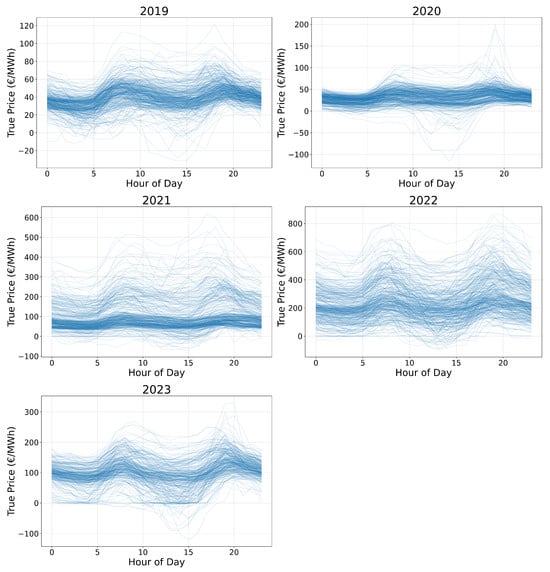
Figure 1. BE electricity price profiles across different years.

Our experimental protocol follows the best practices proposed by [16], which is widely recognized for evaluating forecasting methods in the PEPF domain.

We emphasize that although this benchmark framework is employed here to assess the Moirai model against the D-DNN baseline, it is designed to be extensible. Future work may incorporate additional recent data, exogenous features from ENTSO-E, and other market regions available on the platform, as well as alternative forecasting methodologies.

To construct the datasets, we started from the structured samples provided by [43], covering observations from 2019 to mid-2023. These were further extended by including data from ENTSO-E up to 30 September 2024, thereby matching the temporal span utilized in recent studies investigating D-DNNs under evolving market dynamics (e.g., [44]). The current setup involves hourly day-ahead electricity prices, beyond additional exogenous variables, such as load forecasts and wind/solar generation forecasts. Temporal features, including hour of day and day of week, are encoded using cyclical sine–cosine transformations to accurately capture periodic patterns. All time series have been preprocessed to remove daylight saving time effects. In the SE region, the solar feature has been excluded in previous studies due to unavailability before 2022. Missing single-hour data points were imputed using standard linear interpolation, while daily samples with completely missing features were removed.

For each market, the out-of-sample test period spans a full year, from 1 October 2023 to 30 September 2024, thereby capturing diverse seasonal intervals with distinct characteristics. This evaluation period was selected to provide a clean and forward-looking test set, avoiding overlap with the training data. Notably, the training set encompasses periods of significant market volatility (particularly in 2022 and 2023) driven by geopolitical disruptions such as the Ukrainian conflict, which led to extreme gas price fluctuations and sharp increases in electricity prices, as reflected in Table 3. Incorporating such heterogeneous time periods into the training pipeline aligns with best practices in the recent PEPF literature, where models are evaluated under evolving market dynamics to assess their robustness and adaptability (see, e.g., reference [44] and references therein). This design enables the model to learn from a wide range of price regimes, including both stable and volatile conditions, thereby improving its ability to generalize to future scenarios. While performance metrics for 2022 and 2023 are not reported due to their inclusion in the training data, their presence contributes to the model’s capacity to handle sharp price variations, as demonstrated in its performance on the 2024 test set (see next section). Furthermore, this experimental framework moves beyond previous benchmarks—such as those in [16], which focused on more stable market periods. By evaluating foundation models under current, high-volatility conditions, we provide a more realistic assessment of their operational robustness. Future work will extend this setup to include additional datasets covering broader volatility regimes, supported by the provided open codebase. Moreover, we included the dataset from the original D-DNN paper (see [13,44]), covering the German electricity market over the period 1 January 2015–31 December 2020, with an out-of-sample period spanning from 27 June 2019 to 31 December 2020 (labeled DE20). This enables zero-shot performance comparisons under conditions that are more stable than those of the other datasets. Beyond load and renewable generation forecasts, it involves additional covariates such as EU emission allowance and fossil fuel prices (coal, oil, and natural gas).

The baseline JSU-DNN predictions were obtained following the results reported in [14,45] for the more volatile datasets and DE20, respectively. Predictions for each test set are included in the version v1.0 of the GitHub repository accompanying this work. Additional details regarding accessibility and experiment reproducibility are provided in Appendix A.

2.4. Explored Moirai Configurations

As introduced in Section 1, we first explored the zero-shot Moirai capabilities on the PEPF benchmarks. To this end, the models perform multi-hour inference on a daily basis across the entire test set, incrementally incorporating the previous day’s data into the input context to exploit the most recent information, as in the D-DNN conditioning scheme. During inference for the next day, only hourly information available in the present day (e.g., past price values and day-ahead generation/load forecasts) is provided to avoid data leakage. To form the related input/output batches from the input time series, we adopted a common sliding window approach with a shift of 24 (i.e., 24 hourly) steps.

Zero-shot experiments are initially conducted with a conventional context length of 2048, as ref. [28] reports that performance improvements beyond this threshold are negligible. Subsequently, additional evaluations are performed with context lengths of $\{256,512,1024,2048,4096\}$ to assess the impact of varying historical information on model performance. The patch size is fixed to 32, following the recommendations of [28] for hourly forecasting tasks. Next, the contribution of exogenous variables is examined by excluding them in the zero-shot experiments. Given the well-documented dependence of electricity prices on exogenous features such as load and generation forecasts, this analysis aims to determine whether Moirai leverages these variables to enhance predictive performance. We then assess the zero-shot capabilities on the more stable DE20 task.

Fine-tuning experiments are conducted on the small and base Moirai configurations. The large setup is excluded from the present analysis due to its substantial computational cost and similar zero-shot performance to the base variant, leaving it for future work. Following the D-DNN baseline, this process adopts a recalibration procedure common in the PEPF context, where models are retrained on a weekly basis. Specifically, a rolling window approach is used, where the training data window shifts daily according to the day-ahead forecasting framework. At each recalibration iteration, the models are trained on all available data up to the current day. Then, forecasts are produced for the following week by shifting the context window daily. The recalibration is repeated weekly by advancing the training window accordingly.

Across both settings, training is performed for a maximum of 100 epochs with early stopping (patience = 10), a batch size of 32, and a fixed learning rate of 1 × 10⁻⁴. Other hyperparameters are kept at their default values. Final results, similarly to the D-DNN baseline, are obtained by ensembling five runs with distinct random seeds analyzing both quantile-level and probabilistic aggregation strategies. Output quantiles are derived from 1000 samples generated from the predicted distributions.

All experiments are performed on a workstation equipped with a 12-core Intel Xeon 2265 CPU, 126 GB RAM, and an NVIDIA RTX A5000 GPU.

2.5. Evaluation Metrics

To evaluate the probabilistic performance of the models on the out-of-sample sets, we adopt standard metrics widely used in the PEPF literature [9]. Targeting the general goal of probabilistic forecasting [46]—maximizing sharpness under calibration constraints—we first analyze model calibration by computing the prediction interval coverage probability (PICP) across different coverage levels. Moreover, visual insights into model strengths and weaknesses are provided by calibration plots derived from prediction intervals at fine percentile levels. These plots (presented in Section 3) are organized in a dataset- and model-specific manner to enhance readability and effectively illustrate model calibration across various conditions. Then, we adopt the continuous ranked probability score (CRPS), approximated by the average quantile loss across 99 percentiles, as a proper scoring rule jointly assessing calibration and sharpness of the predictive distribution. The integration of further metrics into the benchmark codebase is planned as part of future extensions, with the goal of providing additional insights. In particular, the Winkler score structures complementary components that reward sharpness and penalize instances where test observations lie outside the predicted interval. Point prediction accuracy is quantified using the mean absolute error (MAE), computed on the 0.5 quantile (median) of the predictive distribution.

To assess the statistical significance of forecast accuracy differences, we employ the model-free Diebold–Mariano (DM) test, which is widely adopted in the PEPF literature (see, e.g., [14,47] and references therein). Complementing conventional metrics that average prediction scores over the dataset, the DM test is based on the pairwise score differentials between forecasts ${\widehat{y}}_d^{M_i}$ and ${\widehat{y}}_d^{M_j}$ generated by competing models $M_i$ and $M_j$ over test days $d=[1,\dots ,N_d]$, followed by an asymptotic z-test assessing the null hypothesis that the expected value of the differential series is zero. The multivariate DM test is performed under a multi-hour forecast framework. Moreover, it facilitates more intuitive visualization of the results via heat maps. Formally, the forecast-score differentials are computed as follows:

$${\mathsf{\Delta }}_d^{M_i,M_j}=\mathcal{L}\left({\epsilon }_d^{M_i}\right)-\mathcal{L}\left({\epsilon }_d^{M_j}\right),\mathrm{with}\mathcal{L}\left({\epsilon }_d^{M_i}\right)={\left(\sum _{h=1}^{24}{\left|{\epsilon }_{d,h}^{M_i}\right|}^n\right)}^{1/n}$$

(14)

where ${\epsilon }_{d,h}^{M_i}=y_{d,h}-{\widehat{y}}_{d,h}^{M_i}\in \mathbb{R}$ is the forecast error at day d and hour h, and $\mathcal{L}$ represents a general n-norm loss function. The DM statistic is then defined as follows:

$${\mathrm{DM}}^{M_i,M_j}=\sqrt{N_d}{\displaystyle \frac{{\widehat{\mu }}^{M_i,M_j}}{{\widehat{\sigma }}^{M_i,M_j}}}$$

(15)

where ${\widehat{\mu }}^{M_i,M_j}$ and ${\widehat{\sigma }}^{M_i,M_j}$ are the sample mean and standard deviation of the differential series ${\mathsf{\Delta }}_d^{M_i,M_j}$ computed over the test period of length $N_d$. In practice, two one-sided tests are conducted, testing the null hypothesis ${\mathrm{H}}_0:\mathbb{E}\left[{\mathsf{\Delta }}_d^{M_i,M_j}\right]\le 0$ against the alternative ${\mathrm{H}}_1:\mathbb{E}\left[{\mathsf{\Delta }}_d^{M_i,M_j}\right]>0$. Rejection of ${\mathrm{H}}_0$ at the conventional 5% significance level indicates that model $M_i$ significantly outperforms model $M_j$.

3. Results Analysis

The upper panels of Figure 2, Figure 3, Figure 4 and Figure 5 report the calibration plots across various nominal coverage levels for the BE, DE, ES, and SE datasets, respectively, using different Moirai architectures with the conventional context length of 2048. In the figure legends, “ZS” denotes zero-shot inference, while “S”, “B”, and “L” correspond to the small, base, and large model architectures. The label “JSU-DNN” refers to the state-of-the-art distributional neural network parameterizing the Johnson’s SU density. Among the zero-shot models, moirai-small exhibits underconfident predictions across the regions, whereas moirai-base and moirai-large display mild overconfidence.

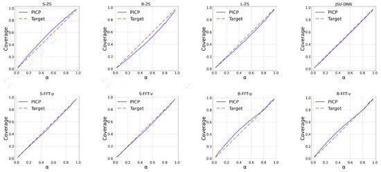
Figure 2. Calibration plots across percentiles for BE region.

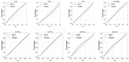
Figure 3. Calibration plots across percentiles for DE region.

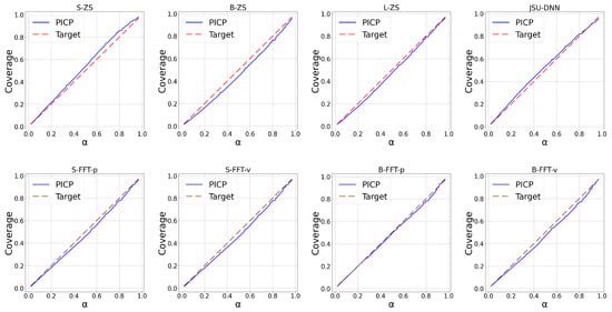
Figure 4. Calibration plots across percentiles for ES region.

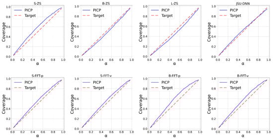
Figure 5. Calibration plots across percentiles for SE_3 region.

Table 4 complements the PICP analysis by reporting mean absolute error (MAE) and continuous ranked probability score (CRPS) performance. Moreover, the PICP values at the conventional coverage level of 1-$\alpha$ = 90% are included, as is common in PEPF studies. Overall, zero-shot forecasts generated by the different Moirai architectures are consistently outperformed by JSU-DNN for both MAE and CRPS metrics. This gap is most pronounced in the DE dataset, while for BE and SE datasets the difference decreases to approximately 15–20%. Within the Moirai configurations, moirai-small exhibits significantly lower accuracy and calibration compared to the moirai-base and moirai-large models, which deliver comparable performance. The statistical significance of the performance difference between the JSU-DNN and Moirai variants, in terms of MAE and CRPS, is confirmed by the results of the Diebold–Mariano (DM) test (see Section 2.5), which are presented in Figure 6. Conversely, no statistically significant difference is observed between the base and large model variants.

Table 4. Out-of-sample results of each model over the 4 regions during 2024.

	BE			DE
Model Name	PICP90%	MAE	CRPS	PICP90%	MAE	CRPS
JSU-DNNp	89.9	13.430	4.846	92.3	10.500	3.808
moirai-small	93.4	18.625	6.875	92.3	19.637	7.293
moirai-base	86.9	16.646	6.106	85.0	17.115	6.323
moirai-large	89.5	16.757	6.159	88.2	16.785	6.205
moirai-small-fftp	92.8	18.391	6.705	92.5	19.284	7.087
moirai-small-fftv	91.9	18.355	6.691	91.9	19.289	7.090
moirai-base-fftp	89.7	19.329	7.091	91.1	20.938	7.794
moirai-base-fftv	84.7	19.317	7.132	86.4	20.899	7.768
	ES			SE_3
Model Name	PICP90%	MAE	CRPS	PICP90%	MAE	CRPS
JSU-DNNp	90.3	11.525	4.252	88.9	11.183	4.151
moirai-small	93.7	16.205	5.953	94.8	15.272	5.728
moirai-base	87.5	14.993	5.482	88.9	13.931	5.225
moirai-large	89.8	14.840	5.443	88.1	13.514	5.090
moirai-small-fftp	92.4	16.504	5.972	92.7	15.165	5.598
moirai-small-fftv	91.6	16.537	5.973	91.9	15.164	5.597
moirai-base-fftp	89.0	18.490	6.647	90.7	16.820	6.309
moirai-base-fftv	79.7	18.668	6.789	86.2	16.846	6.312

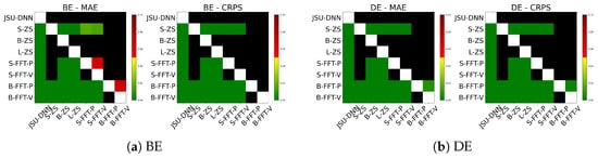
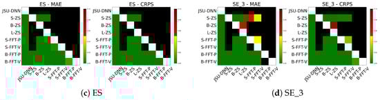
Figure 6. DM test on MAE and CRPS for each market region.

Table 5 and Table 6 present the test metrics for the winter period (December 2023–February 2024) and the summer period (June 2024–August 2024), highlighting performance sensitivity across seasonal variations and heterogeneous regional market conditions characterized by specific volatility levels. Notably, in the SE_3 market (characterized by lower average price values as reported in Section 2.3), all models perform better during summer, while in the other regions, the models show higher scores overall. The discrepancies between the specialized model and Moirai remain comparable to those reported in the full-year evaluation in Table 4. Regarding PICP, the JSU-DNN is close to the target values in both periods, while the Moirai models—especially the small variant—exhibit reduced calibration compared to the full-year results. These observations are motivated by region-specific changes in price settlement across different bidding zones (e.g., the cold winter in Sweden affecting power demand). Still, more profound sensitivity analyses, such as examining additional time horizons and market regimes, represent valuable directions for future works.

Table 5. Out-of-sample results of each model over the 4 regions during winter 2024.

	BE			DE
ModelName	PICP90%	MAE	CRPS	PICP90%	MAE	CRPS
JSU-DNNp	90.1	8.709	3.120	92.3	7.092	2.612
moirai-small	98.4	12.251	4.595	97.8	13.173	4.899
moirai-base	94.0	10.921	3.883	93.3	11.418	4.076
moirai-large	90.0	10.302	3.750	88.9	11.100	4.018
moirai-small-fftp	97.6	11.183	4.017	98.6	11.919	4.411
moirai-small-fftv	97.3	11.204	4.010	98.5	11.928	4.397
moirai-base-fftp	96.9	12.811	4.695	97.4	13.523	4.853
moirai-base-fftv	92.4	12.834	4.619	91.9	13.814	4.865
	ES			SE_3
Model Name	PICP90%	MAE	CRPS	PICP90%	MAE	CRPS
JSU-DNNp	89.8	9.920	3.641	86.7	14.908	5.591
moirai-small	94.1	13.285	4.917	96.0	18.776	7.085
moirai-base	88.1	13.813	4.932	89.3	16.696	6.336
moirai-large	89.2	13.840	4.997	85.3	16.925	6.479
moirai-small-fftp	94.4	13.412	4.883	94.0	17.337	6.558
moirai-small-fftv	93.7	13.417	4.874	92.4	17.277	6.537
moirai-base-fftp	88.8	18.055	6.517	95.4	21.366	7.798
moirai-base-fftv	75.3	17.667	6.563	91.5	21.141	7.726

Table 6. Out-of-sample results of each model over the 4 regions during summer 2024.

	BE			DE
Model Name	PICP90%	MAE	CRPS	PICP90%	MAE	CRPS
JSU-DNNp	91.5	14.674	5.277	92.8	11.492	4.162
moirai-small	92.3	20.405	7.439	90.3	21.450	8.030
moirai-base	86.8	17.845	6.459	83.0	17.863	6.563
moirai-large	93.5	17.465	6.363	92.8	17.762	6.420
moirai-small-fftp	93.7	19.918	7.177	92.1	20.510	7.580
moirai-small-fftv	93.2	19.891	7.171	90.8	20.500	7.595
moirai-base-fftp	90.6	20.745	7.465	91.4	20.012	7.376
moirai-base-fftv	84.1	20.602	7.545	86.8	20.361	7.460
	ES			SE_3
Model Name	PICP90%	MAE	CRPS	PICP90%	MAE	CRPS
JSU-DNNp	94.2	11.671	4.345	90.6	6.313	2.324
moirai-small	93.4	17.592	6.576	96.6	8.036	3.042
moirai-base	87.2	16.349	5.948	89.7	7.393	2.770
moirai-large	92.0	14.992	5.467	90.7	7.110	2.675
moirai-small-fftp	93.6	17.909	6.431	93.0	7.914	2.986
moirai-small-fftv	93.0	17.935	6.428	92.5	7.914	2.981
moirai-base-fftp	87.9	18.459	6.713	95.5	8.908	3.319
moirai-base-fftv	78.0	18.925	6.907	92.5	8.707	3.207

Table 7 presents the results across different context lengths. The analysis shows that no single configuration uniformly optimizes performance; rather, the optimal window size varies depending on both the dataset and the model scale. In our experiments, smaller models such as moirai-small achieve the best MAE and CRPS with shorter windows around 512, while larger models, moirai-base and moirai-large, benefit from progressively longer context lengths of 1024 and 2048 or greater, respectively. Similar trends are observed in calibration metrics. Specifically, moirai-small achieves better PICP values with shorter context lengths (256 and 512), while moirai-base and moirai-large achieve improved calibration at longer windows (2048 and 4096). Figure 7 and Figure 8 display the respective Diebold–Mariano test results. For moirai-small, context lengths of 256, 512, and 1024 significantly outperform longer windows (2048 and 4096), with no significant differences among these shorter intervals. In contrast, for moirai-base and moirai-large, windows exceeding 256 provide significantly better predictive performance, while no significant difference is found between 2048 and 4096.

Table 7. Out-of-sample zero-shot results across all regions for different context lengths.

		BE			DE
Model Name	Context Size	PICP90%	MAE	CRPS	PICP90%	MAE	CRPS
moirai-small	256	90.3	18.760	6.860	89.4	19.750	7.261
moirai-small	512	91.0	18.602	6.804	90.3	19.514	7.188
moirai-small	1024	92.0	18.606	6.833	91.2	19.513	7.213
moirai-small	2048	93.4	18.625	6.875	92.3	19.637	7.293
moirai-small	4096	95.1	19.151	7.116	94.2	20.213	7.531
moirai-base	256	85.0	17.889	6.561	82.3	18.736	6.939
moirai-base	512	86.2	16.782	6.156	83.9	17.503	6.435
moirai-base	1024	86.5	16.582	6.086	84.4	17.107	6.306
moirai-base	2048	86.9	16.646	6.106	85.0	17.115	6.323
moirai-base	4096	87.7	16.661	6.104	86.5	17.222	6.347
moirai-large	256	89.2	17.497	6.456	87.8	17.757	6.626
moirai-large	512	89.8	16.836	6.216	88.1	16.931	6.299
moirai-large	1024	89.4	16.772	6.181	88.2	16.727	6.203
moirai-large	2048	89.5	16.757	6.159	88.2	16.785	6.205
moirai-large	4096	89.6	16.855	6.189	88.5	17.060	6.279
		ES			SE_3
Model Name	Context Size	PICP90%	MAE	CRPS	PICP90%	MAE	CRPS
moirai-small	256	90.0	15.763	5.835	91.1	14.492	5.456
moirai-small	512	91.5	15.687	5.765	92.7	14.611	5.504
moirai-small	1024	92.6	15.868	5.845	93.9	14.831	5.575
moirai-small	2048	93.7	16.205	5.953	94.8	15.272	5.728
moirai-small	4096	94.4	16.663	6.112	96.2	16.102	5.999
moirai-base	256	84.2	15.247	5.672	81.8	13.965	5.316
moirai-base	512	85.7	14.704	5.444	84.3	13.598	5.114
moirai-base	1024	86.8	14.586	5.359	86.9	13.754	5.153
moirai-base	2048	87.5	14.993	5.482	88.9	13.931	5.225
moirai-base	4096	87.4	15.067	5.524	91.4	13.877	5.225
moirai-large	256	87.6	15.314	5.659	83.8	13.994	5.318
moirai-large	512	88.8	14.838	5.459	85.7	13.665	5.163
moirai-large	1024	89.9	14.794	5.425	87.4	13.612	5.106
moirai-large	2048	89.8	14.840	5.443	88.1	13.514	5.090
moirai-large	4096	89.9	14.906	5.464	89.2	13.604	5.130

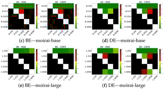
Figure 7. DM test on MAE and CRPS for various context lengths in BE and DE regions.

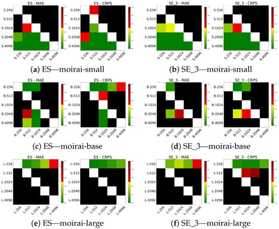
Figure 8. DM test on MAE and CRPS for various context lengths in ES and SE_3 regions.

Table 8 presents zero-shot forecast performance when excluding exogenous variables, i.e., conditioning only on hourly price values within the context. Notably, for the BE, ES, and SE markets, both moirai-small and moirai-large exhibit improved MAE and CRPS relative to their covariate-informed counterparts, while moirai-base shows a performance decline. In the DE market, improvements from excluding exogenous inputs are observed only for moirai-large. Surprisingly, dropping exogenous variables leads all Moirai architectures to achieve coverage probabilities closer to the nominal level across the different regions. Diebold–Mariano (DM) tests results are reported in Figure 9, showing that moirai-small without covariates significantly outperforms its covariate-enabled version only in the SE market. Conversely, moirai-base deteriorates markedly, underperforming even moirai-small. In contrast, moirai-large consistently yields statistically significant improvements over its covariate-enabled configuration across all regions for both MAE and CRPS.

Table 8. Out-of-sample zero-shot results excluding both past and future exogenous variables.

Model Name	Market	Covariates	PICP90%	MAE	CRPS
moirai-small	BE	Yes	93.4	18.625	6.875
moirai-small	BE	No	91.8	18.760	6.839
moirai-base	BE	Yes	86.9	16.646	6.106
moirai-base	BE	No	88.2	19.514	7.196
moirai-large	BE	Yes	89.5	16.757	6.159
moirai-large	BE	No	90.2	16.106	5.866
moirai-small	DE	Yes	92.3	19.637	7.293
moirai-small	DE	No	90.8	20.260	7.416
moirai-base	DE	Yes	85.0	17.115	6.323
moirai-base	DE	No	90.6	20.155	7.432
moirai-large	DE	Yes	88.2	16.785	6.205
moirai-large	DE	No	88.3	16.266	5.980
moirai-small	ES	Yes	93.7	16.205	5.953
moirai-small	ES	No	90.8	15.889	5.843
moirai-base	ES	Yes	87.5	14.993	5.482
moirai-base	ES	No	88.6	16.839	6.155
moirai-large	ES	Yes	89.8	14.840	5.443
moirai-large	ES	No	89.6	13.985	5.131
moirai-small	SE_3	Yes	94.8	15.272	5.728
moirai-small	SE_3	No	92.8	14.755	5.561
moirai-base	SE_3	Yes	88.9	13.931	5.225
moirai-base	SE_3	No	92.9	14.541	5.428
moirai-large	SE_3	Yes	88.1	13.514	5.090
moirai-large	SE_3	No	88.2	13.063	4.925

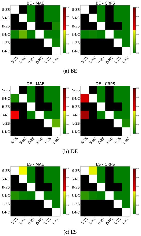
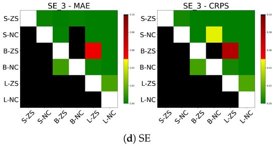
Figure 9. DM test on MAE and CRPS for the results excluding both past and future exogenous variables.

Table 9 reports results on the DE20 dataset, which features more stationary market conditions, aimed to assess whether reduced volatility impacts model behavior. The relative performance gap between Moirai zero-shot forecasts and JSU-DNN predictions exhibits a magnitude comparable to that observed in previously reported, more volatile, DE experiments. Additional insights are obtained by inspecting Table 10, reporting PICP values across different confidence levels. moirai-small maintain underconfident outputs, while the larger Moirai models demonstrate slightly better calibration than JSU-DNN. Figure 10 further supports these observations by the Diebold–Mariano test results, where JSU-DNN significantly outperforms all Moirai zero-shot variants on DE20. Performance scaling with model size persists, with larger Moirai models consistently outperforming smaller architectures.

Table 9. Out-of-sample results of JSU-DNN and zero-shot models over the stationary DE20 dataset.

Model Name	PICP80%	MAE	CRPS
JSU-DNN	73.3	3.724	1.467
moirai-small	85.2	7.432	3.003
moirai-base	77.6	6.223	2.522
moirai-large	77.2	5.895	2.392

Table 10. PICP results in % for different confidence levels $\left(\alpha \right)$ over the stationary DE20 dataset.

	Moirai-Small	Moirai-Base	Moirai-Large	JSU-DNN
PICP (α = 0.2)	24.5	18.4	18.4	17.2
PICP (α = 0.4)	47.4	36.8	37.2	35.3
PICP (α = 0.6)	67.8	56.7	56.7	53.8
PICP (α = 0.8)	85.2	77.6	77.2	73.7

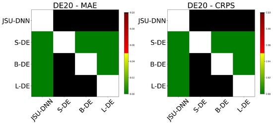
Figure 10. DM test on MAE and CRPS over the stationary DE20 dataset.

The results of the fine-tuning experiments are reported in the tables and figures with the label “FFT” standing for “Full Fine Tuning”. Labels p and v indicate the alternative ensemble strategies applied on the generated prediction samples, based on probability aggregation and quantile averaging (also known as Vincentization [48]), respectively. Notably, the fine-tuned moirai-small architectures show sensibly improved calibration, approaching target coverage across multiple degrees. In contrast, moirai-base transitions from overconfidence to underconfidence after fine-tuning, suggesting potential overfitting given the model’s relatively large capacity and the limited size of the fine-tuning datasets. By comparison, the JSU-DNN ensemble achieves well-calibrated predictive intervals across all market regions. The two aggregation strategies do not exhibit a consistent pattern of improvement; gains in favor of one approach depend on the specific dataset. For moirai-small, fine-tuning followed by ensemble aggregation yields modest improvements over the zero-shot baseline, while for moirai-base, performance deteriorates relative to its zero-shot counterpart. The Diebold–Mariano tests confirm the statistical significance of the performance improvement observed for fine-tuned moirai-small and the performance degradation for fine-tuned moirai-base. Still, exploration of alternative fine-tuning strategies constitutes a compelling direction for future work.

To provide additional insights into the models’ behavior beyond average performance metrics, Figure 11a–d present zero-shot predictions on test samples across different model sizes. Specifically, the 99 output quantiles over a seven-day horizon, corresponding to a randomly selected week from Monday through Sunday, are shown. Prediction intervals vary in sharpness, with moirai-small exhibiting the widest average bands, while the two larger models display comparable behavior. Furthermore, Figure 12a–d compare the best-performing zero-shot moirai-large configuration with the JSU-DNN baseline. The forecasts produced by Moirai show a high degree of coherence with those of the domain-specific model, indicating a sensible capacity to capture the intrinsic temporal dynamics of the price series. However, notable deviations occur during pronounced daily peaks and transitions to lower regimes, where Moirai presents substantially broader confidence intervals and struggles to capture steep daily price fluctuations.

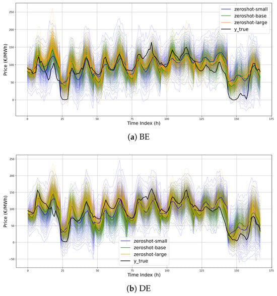
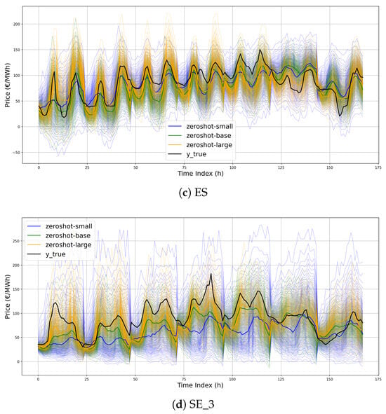
Figure 11. Illustration of the 99 forecast quantiles for the zero-shot models over the entire week starting from Monday 12 November 2023.

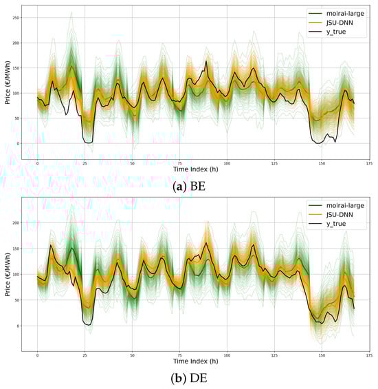
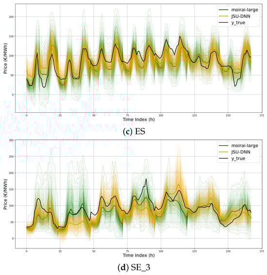
Figure 12. Illustration of the 99 forecast quantiles for JSU-DNN and moirai-large over the entire week starting from Monday 12 November 2023.

4. Discussion

Despite the reported gap in performance metrics relative to the specialized JSU-DNN model for PEPF, the zero-shot capabilities of Moirai remain highly promising, warranting further exploration of TSFM in this context. Isolated large forecast errors, such as the anomalous price spike predicted by Moirai at the end of the first day of DE market in Figure 12 (zoomed in Figure 13), may sensibly impact average test set performance metrics. Conversely, on some days, it appears to provide even better predictions (see, e.g., the second day in the SE_3 market in Figure 12, zoomed in Figure 14). Improved handling of exogenous information could be crucial in this context. While the specialized D-DNN baseline has been shown to effectively exploit relationships between auxiliary covariates and the target series (see, e.g., [8,44]), the experimented Moirai configurations appear not to benefit from their integration. Both the D-DNN baseline and the Moirai architecture were provided with consistent conditioning features and lag coverage from past series. Internally, Moirai applies instance normalization [49] to inputs/outputs, aligning with the current standard practice for deep forecasting models [28]. The D-DNN applies the same procedure. However, a more detailed assessment of the impact of specific feature selection, lag structuring, and different normalization techniques (e.g., methods for handling extreme values in the input series) deserves further investigation in future studies. Moreover, Moirai’s relatively lower performance compared to specialized D-DNNs may be attributed to several interrelated factors. Firstly, its architecture, designed for broad generalization across diverse time series domains, employs flexible mechanisms rather than fixed inductive biases for capturing specific seasonal patterns or abrupt regime shifts, which may limit its ability to exploit domain-specific features fully. Secondly, although Moirai is pretrained on an extensive corpus, this data may not comprehensively encompass the volatility patterns and structural complexities unique to power markets. Additionally, prevailing fine-tuning protocols for TSFMs emphasize parameter efficiency; while computationally advantageous, this may constrain the degree of domain-specific adaptation achieved.

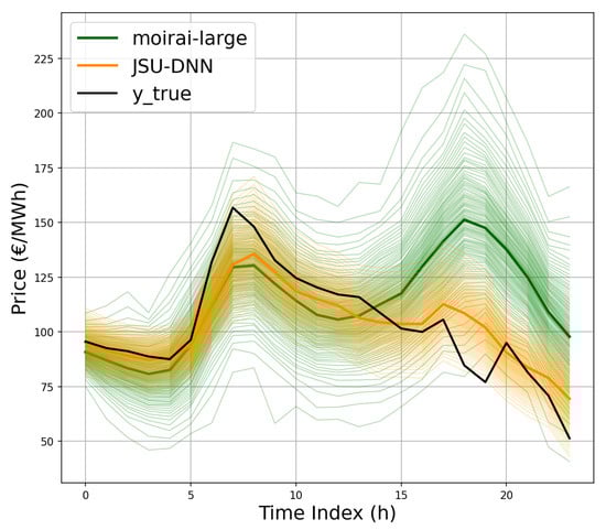
Figure 13. Example of isolated large forecast error by Moirai, at the end of the first day of the week (DE market).

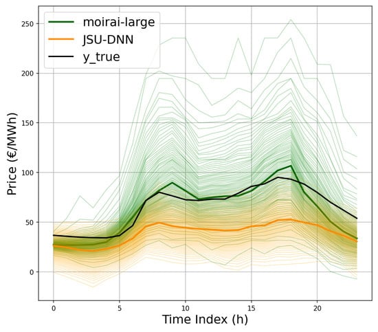
Figure 14. Example of accurate prediction by Moirai during the second day of the week (SE_3 market).

To summarize, Table 11 highlights the main strengths and limitations observed in the deployed specialized D-DNNs and Moirai TSFM, which pose challenges for future developments.

Table 11. Overall comparison between specialized D-DNNs and Moirai.

	D-DNN	Moirai
Performance	Better probabilistic scores with proper calibration.	Worse performance with mild miscalibration.
Cross-task (e.g., markets)	Limited; requires full retraining.	High; supports zero/few-shot forecasting.
Feature control	Full design control.	TSFM model dependent.
Tackle steep fluctuations	High, due to dataset specific learning.	Limited under pronounced transitions.
Training costs	Low–moderate.	Very high (only pretrain).
Data Requirements	Targeted, labeled datasets.	Massive pretraining corpora.
Inference	Fast and low-cost.	Slower and more expansive at scale.

Promising directions for improvement include architectural enhancements integrating domain-specific priors, the creation of large-scale and synthetic datasets tailored to electricity markets, and fine-tuning strategies that better balance efficiency with deeper adaptation. Advances in these areas are expected to narrow the performance gap and enable foundation models to compete more effectively with specialized architectures in PEPF.

5. Conclusions

The main scope of this work was to contribute to the further understanding of time series foundation models (TSFMs) applied to challenging probabilistic electricity price forecasting (PEPF) tasks. We focused on the Moirai model, providing an open-source probabilistic framework with native covariate support and fine-tuning capabilities, enabling a rigorous comparison against state-of-the-art specialized neural networks. We established a comprehensive open benchmark using data from the ENTSO-E transparency platform across multiple regions to capture heterogeneous market conditions. Our experimental protocol adhered to best practices in PEPF evaluation, analyzing probabilistic forecast accuracy with the CRPS proper scoring rule and calibration via PICP reliability analysis across various coverage levels. This analysis is essential, as the primary objective of probabilistic forecasting is to achieve maximum sharpness while guaranteeing proper calibration. Additionally, we used the model-free Diebold–Mariano test to assess the statistical significance of forecast differences. As a specialized baseline, we implemented a distributional neural network (D-DNN) parameterizing a flexible Johnson’s SU density. A systematic analysis of Moirai architectures was performed under zero-shot and fine-tuning scenarios.

Our results show that although Moirai currently underperforms specialized D-DNNs on probabilistic metrics, it effectively captures intrinsic temporal dynamics in price series. Prediction challenges remain during sharp daily peaks and regime shifts, where Moirai struggles with steep fluctuations. Despite its principled ability to leverage exogenous inputs, we observed limited—and in some cases even detrimental—impacts on forecasting performance resulting from their integration. Addressing these issues represents a significant avenue for future research.

In conclusion, we acknowledge that this study is not exhaustive, as numerous practical aspects remain to be explored. First, we aim to broaden the empirical scope of the benchmark by incorporating additional datasets that capture a wider range of volatility regimes and market conditions. This includes integrating exogenous features from sources such as ENTSO-E and extending the analysis to other market regions. We also plan to refine data preprocessing and transformation pipelines, paying particular attention to input conditioning and lag structures. Next, we will conduct a more in-depth sensitivity analysis, incorporating additional metrics, to assess model robustness across various forecast horizons (including intraday and long-term forecasts) under changing regimes. Subsequently, we intend to explore alternative architectural designs, such as transformer-based models, hybrid ensembles, and different output parameterizations (e.g., distributional forecasting versus quantile regression). Finally, we envision the exploration of novel TSFM architectures, advanced fine-tuning strategies, and global models specifically tailored for PEPF tasks. Addressing these challenges exceeds the scope of a single study and requires a coordinated effort from the research community. Our analysis represents only one step in this ongoing process, and we hope that the benchmark we have established, along with future extensions, will help foster progress in this direction.

Ultimately, TSFMs should be viewed not as replacements for specialized forecasting models but as complementary tools within a broader forecasting toolkit. The choice of forecasting methods depends on both technical and economic factors, including the availability of specialized personnel and the economic value tied to the specific time series. Moreover, AI-driven forecasting in energy markets amplifies existing ethical challenges related to transparency, fairness, and data privacy. This study relies exclusively on publicly available data from ENTSO-E, ensuring transparency and avoiding privacy issues. However, models that incorporate proprietary or internal operational data face heightened privacy and fairness concerns. Explainability and accountability must be prioritized throughout model development and deployment. Addressing these issues calls for robust frameworks, continuing research, and systematic fairness audits. Responsible AI adoption in energy forecasting hinges on aligning technological innovation with societal values and regulatory standards, supporting a sustainable energy future. Given the substantial impact of energy price forecasts on large companies within the value chain, the continued use of highly specialized models is expected. Nevertheless, TSFMs may provide valuable benchmarking capabilities for achievable performance levels, guiding further model development and potential integration within ensemble approaches. Moreover, PEPF offers a compelling testbed for evaluating the evolving capabilities of TSFMs, providing an informative environment for their deployment in contexts where economic and technical factors support the adoption of these innovative zero- and few-shot learning tools.

References

- Arroyo, J.M.; Conejo, A.J. Optimal response of a thermal unit to an electricity spot market. IEEE Trans. Power Syst. 2002, 15, 1098–1104. [Google Scholar] [CrossRef]
- Fleten, S.E.; Kristoffersen, T.K. Stochastic programming for optimizing bidding strategies of a Nordic hydropower producer. Eur. J. Oper. Res. 2007, 181, 916–928. [Google Scholar] [CrossRef]
- Weron, R. Electricity price forecasting: A review of the state-of-the-art with a look into the future. Int. J. Forecast. 2014, 30, 1030–1081. [Google Scholar] [CrossRef]
- Prokhorov, O.; Dreisbach, D. The impact of renewables on the incidents of negative prices in the energy spot markets. Energy Policy 2022, 167, 113073. [Google Scholar] [CrossRef]
- Zakeri, B.; Staffell, I.; Dodds, P.E.; Grubb, M.; Ekins, P.; Jääskeläinen, J.; Cross, S.; Helin, K.; Gissey, G.C. The role of natural gas in setting electricity prices in Europe. Energy Rep. 2023, 10, 2778–2792. [Google Scholar] [CrossRef]
- Hyndman, R.; Koehler, A.B.; Ord, J.K.; Snyder, R.D. Forecasting with Exponential Smoothing: The State Space Approach; Springer Science & Business Media: Berlin/Heidelberg, Germany, 2008. [Google Scholar]
- Aggarwal, S.K.; Saini, L.M.; Kumar, A. Electricity price forecasting in deregulated markets: A review and evaluation. Int. J. Electr. Power Energy Syst. 2009, 31, 13–22. [Google Scholar] [CrossRef]
- Mashlakov, A.; Kuronen, T.; Lensu, L.; Kaarna, A.; Honkapuro, S. Assessing the performance of deep learning models for multivariate probabilistic energy forecasting. Appl. Energy 2021, 285, 116405. [Google Scholar] [CrossRef]
- Nowotarski, J.; Weron, R. Recent advances in electricity price forecasting: A review of probabilistic forecasting. Renew. Sustain. Energy Rev. 2018, 81, 1548–1568. [Google Scholar] [CrossRef]
- Brusaferri, A.; Matteucci, M.; Portolani, P.; Vitali, A. Bayesian deep learning based method for probabilistic forecast of day-ahead electricity prices. Appl. Energy 2019, 250, 1158–1175. [Google Scholar] [CrossRef]
- Wagner, A.; Ramentol, E.; Schirra, F.; Michaeli, H. Short- and long-term forecasting of electricity prices using embedding of calendar information in neural networks. J. Commod. Mark. 2022, 28, 100246. [Google Scholar] [CrossRef]
- Ramin, D.; Spinelli, S.; Brusaferri, A. Demand-side management via optimal production scheduling in power-intensive industries: The case of metal casting process. Appl. Energy 2018, 225, 622–636. [Google Scholar] [CrossRef]
- Marcjasz, G.; Narajewski, M.; Weron, R.; Ziel, F. Distributional neural networks for electricity price forecasting. Energy Econ. 2023, 125, 106843. [Google Scholar] [CrossRef]
- Brusaferri, A.; Ballarino, A.; Grossi, L.; Laurini, F. On-line conformalized neural networks ensembles for probabilistic forecasting of day-ahead electricity prices. Appl. Energy 2025, 398, 126412. [Google Scholar] [CrossRef]
- Lago, J.; De Ridder, F.; De Schutter, B. Forecasting spot electricity prices: Deep learning approaches and empirical comparison of traditional algorithms. Appl. Energy 2018, 221, 386–405. [Google Scholar] [CrossRef]
- Lago, J.; Marcjasz, G.; De Schutter, B.; Weron, R. Forecasting day-ahead electricity prices: A review of state-of-the-art algorithms, best practices and an open-access benchmark. Appl. Energy 2021, 293, 116983. [Google Scholar] [CrossRef]
- Vaswani, A.; Shazeer, N.; Parmar, N.; Uszkoreit, J.; Jones, L.; Gomez, A.N.; Kaiser, Ł.; Polosukhin, I. Attention is all you need. Adv. Neural Inf. Process. Syst. 2017, 30, 6000–6010. [Google Scholar]
- Salinas, D.; Flunkert, V.; Gasthaus, J.; Januschowski, T. DeepAR: Probabilistic forecasting with autoregressive recurrent networks. Int. J. Forecast. 2020, 36, 1181–1191. [Google Scholar] [CrossRef]
- Oreshkin, B.N.; Carpov, D.; Chapados, N.; Bengio, Y. N-BEATS: Neural basis expansion analysis for interpretable time series forecasting. arXiv 2019, arXiv:1905.10437. [Google Scholar]
- Das, A.; Kong, W.; Leach, A.; Mathur, S.; Sen, R.; Yu, R. Long-term forecasting with tide: Time-series dense encoder. arXiv 2023, arXiv:2304.08424. [Google Scholar]
- Olivares, K.G.; Challu, C.; Marcjasz, G.; Weron, R.; Dubrawski, A. Neural basis expansion analysis with exogenous variables: Forecasting electricity prices with NBEATSx. Int. J. Forecast. 2023, 39, 884–900. [Google Scholar] [CrossRef]
- Yu, R.; Gu, C.; Stiasny, J.; Wen, Q.; Dilov, W.S.; Qi, L.; Cremer, J.L. Pricefm: Foundation model for probabilistic electricity price forecasting. arXiv 2025, arXiv:2508.04875. [Google Scholar] [CrossRef]
- Lei, X.; Yu, H.; Yu, B.; Shao, Z.; Jian, L. Bridging electricity market and carbon emission market through electric vehicles: Optimal bidding strategy for distribution system operators to explore economic feasibility in China’s low-carbon transitions. Sustain. Cities Soc. 2023, 94, 104557. [Google Scholar] [CrossRef]
- Xue, H.; Salim, F.D. Promptcast: A new prompt-based learning paradigm for time series forecasting. IEEE Trans. Knowl. Data Eng. 2023, 36, 6851–6864. [Google Scholar] [CrossRef]
- Gruver, N.; Finzi, M.; Qiu, S.; Wilson, A.G. Large language models are zero-shot time series forecasters. Adv. Neural Inf. Process. Syst. 2023, 36, 19622–19635. [Google Scholar]
- Zhou, T.; Niu, P.; Sun, L.; Jin, R. One fits all: Power general time series analysis by pretrained lm. Adv. Neural Inf. Process. Syst. 2023, 36, 43322–43355. [Google Scholar]
- Jin, M.; Wang, S.; Ma, L.; Chu, Z.; Zhang, J.Y.; Shi, X.; Chen, P.Y.; Liang, Y.; Li, Y.F.; Pan, S.; et al. Time-LLM: Time series forecasting by reprogramming large language models. In Proceedings of the International Conference on Learning Representations (ICLR), Vienna, Austria, 7–11 May 2024. [Google Scholar]
- Woo, G.; Liu, C.; Kumar, A.; Xiong, C.; Savarese, S.; Sahoo, D. Unified training of universal time series forecasting transformers. In Proceedings of the 41st International Conference on Machine Learning, PMLR, Vienna, Austria, 21–27 August 2024. [Google Scholar]
- Ansari, A.F.; Stella, L.; Turkmen, C.; Zhang, X.; Mercado, P.; Shen, H.; Shchur, O.; Rangapuram, S.S.; Arango, S.P.; Kapoor, S.; et al. Chronos: Learning the language of time series. arXiv 2024, arXiv:2403.07815. [Google Scholar] [CrossRef]
- Aksu, T.; Woo, G.; Liu, J.; Liu, X.; Liu, C.; Savarese, S.; Xiong, C.; Sahoo, D. GIFT-Eval: A Benchmark for General Time Series Forecasting Model Evaluation. In Proceedings of the NeurIPS Workshop on Time Series in the Age of Large Models, Vancouver, BC, Canada, 15 December 2024. [Google Scholar]
- Shchur, O.; Ansari, A.F.; Turkmen, C.; Stella, L.; Erickson, N.; Guerron, P.; Bohlke-Schneider, M.; Wang, Y. fev-bench: A Realistic Benchmark for Time Series Forecasting. arXiv 2025, arXiv:2509.26468. [Google Scholar] [CrossRef]
- Wang, Y.; Wu, H.; Dong, J.; Qin, G.; Zhang, H.; Liu, Y.; Qiu, Y.; Wang, J.; Long, M. Timexer: Empowering transformers for time series forecasting with exogenous variables. Adv. Neural Inf. Process. Syst. 2024, 37, 469–498. [Google Scholar]
- ENTSO-E Transparency Platform. 2025. Available online: https://transparency.entsoe.eu/ (accessed on 24 October 2025).
- Rasul, K.; Ashok, A.; Williams, A.R.; Ghonia, H.; Bhagwatkar, R.; Khorasani, A.; Bayazi, M.J.D.; Adamopoulos, G.; Riachi, R.; Hassen, N.; et al. Lag-Llama: Towards Foundation Models for Probabilistic Time Series Forecasting. arXiv 2024, arXiv:2310.08278. [Google Scholar] [CrossRef]
- Raffel, C.; Shazeer, N.; Roberts, A.; Lee, K.; Narang, S.; Matena, M.; Zhou, Y.; Li, W.; Liu, P.J. Exploring the limits of transfer learning with a unified text-to-text transformer. J. Mach. Learn. Res. 2020, 21, 5485–5551. [Google Scholar]
- Das, A.; Kong, W.; Sen, R.; Zhou, Y. A decoder-only foundation model for time-series forecasting. In Proceedings of the Forty-First International Conference on Machine Learning, Vienna, Austria, 21–27 July 2024. [Google Scholar]
- Cohen, B.; Khwaja, E.; Doubli, Y.; Lemaachi, S.; Lettieri, C.; Masson, C.; Miccinilli, H.; Ramé, E.; Ren, Q.; Rostamizadeh, A.; et al. This Time is Different: An Observability Perspective on Time Series Foundation Models. arXiv 2025, arXiv:2505.14766. [Google Scholar] [CrossRef]
- Ekambaram, V.; Jati, A.; Dayama, P.; Mukherjee, S.; Nguyen, N.H.; Gifford, W.M.; Reddy, C.; Kalagnanam, J. Tiny Time Mixers (TTMs): Fast Pre-trained Models for Enhanced Zero/Few-Shot Forecasting of Multivariate Time Series. In Proceedings of the Advances in Neural Information Processing Systems (NeurIPS 2024), Vancouver, BC, Canada, 10–15 December 2024. [Google Scholar]
- Hoo, S.B.; Müller, S.; Salinas, D.; Hutter, F. The tabular foundation model TabPFN outperforms specialized time series forecasting models based on simple features. In Proceedings of the NeurIPS Workshop on Time Series in the Age of Large Models, Vancouver, BC, Canada, 15 December 2024. [Google Scholar]
- Goswami, M.; Szafer, K.; Choudhry, A.; Cai, Y.; Li, S.; Dubrawski, A. Moment: A family of open time-series foundation models. arXiv 2024, arXiv:2402.03885. [Google Scholar] [CrossRef]
- Garza, A.; Mergenthaler-Canseco, M. TimeGPT-1. arXiv 2023, arXiv:2310.03589. [Google Scholar] [CrossRef]
- Kottapalli, S.R.K.; Hubli, K.; Chandrashekhara, S.; Jain, G.; Hubli, S.; Botla, G.; Doddaiah, R. Foundation Models for Time Series: A Survey. arXiv 2025, arXiv:2504.04011. [Google Scholar] [CrossRef]
- Aliyon, K.; Ritvanen, J. Deep learning-based electricity price forecasting: Findings on price predictability and European electricity markets. Energy 2024, 308, 132877. [Google Scholar] [CrossRef]
- Brusaferri, A.; Ramin, D.; Ballarino, A. From Distributional to Quantile Neural Basis Models: The case of Electricity Price Forecasting. arXiv 2025, arXiv:2509.14113. [Google Scholar] [CrossRef]
- Brusaferri, A.; Ramin, D.; Ballarino, A. NBMLSS: Probabilistic forecasting of electricity prices via Neural Basis Models for Location Scale and Shape. arXiv 2024, arXiv:2411.13921. [Google Scholar] [CrossRef]
- Gneiting, T.; Raftery, A.E. Strictly Proper Scoring Rules, Prediction, and Estimation. J. Am. Stat. Assoc. 2007, 102, 359–378. [Google Scholar] [CrossRef]
- Tschora, L.; Pierre, E.; Plantevit, M.; Robardet, C. Electricity price forecasting on the day-ahead market using machine learning. Appl. Energy 2022, 313, 118752. [Google Scholar] [CrossRef]
- Lichtendahl, K.C.; Grushka-Cockayne, Y.; Winkler, R.L. Is It Better to Average Probabilities or Quantiles? Manag. Sci. 2013, 59, 1594–1611. [Google Scholar] [CrossRef]
- Kim, T.; Kim, J.; Tae, Y.; Park, C.; Choi, J.H.; Choo, J. Reversible Instance Normalization for Accurate Time-Series Forecasting against Distribution Shift. In Proceedings of the International Conference on Learning Representations, Virtual, 3–7 May 2021. [Google Scholar]
Disclaimer/Publisher’s Note: The statements, opinions and data contained in all publications are solely those of the individual author(s) and contributor(s) and not of MDPI and/or the editor(s). MDPI and/or the editor(s) disclaim responsibility for any injury to people or property resulting from any ideas, methods, instructions or products referred to in the content. |
© 2025 by the authors. Licensee MDPI, Basel, Switzerland. This article is an open access article distributed under the terms and conditions of the Creative Commons Attribution (CC BY) license (https://creativecommons.org/licenses/by/4.0/).