Design Scenarios and Risk-Aware Performance Framework for Modular EV Fast Charging Stations

Abstract

The rapid growth of electric vehicles (EVs) requires the deployment of modular fast charging stations that balance charging performance, grid limitations, and investment costs. This study develops design scenarios for modular EV fast charging stations and introduces a risk-aware performance analysis framework under power and grid quality constraints. A simulation-based approach evaluates 286 station configurations with ten charging outlets (20–50 kW), grouped into 16 representative classes based on three key dimensions: total installed power, dominant charger type, and peak load risk. Performance metrics such as efficiency of charger utilization, load factor, and overload risk are used to construct Pareto frontiers and identify optimal trade-offs between capacity and operational safety. Results indicate that medium-power configurations (251–350 kW) achieve the best compromise between efficiency (>82%) and load factor (>50%) without exceeding safe operating limits, while high-power configurations enable maximum throughput at the expense of elevated overload risk. Sensitivity analysis confirms the robustness of the proposed grouping approach under variations in arrival rates, battery sizes, and grid constraints (400–600 kW). The findings provide practical insights into the design and risk management of modular charging stations, supporting urban planners and power engineers in developing efficient and reliable EV charging infrastructure.

1. Introduction

The expanding use of electric vehicles (EVs) in recent years has positioned them as an essential element of sustainable urban mobility. Their main advantages, such as zero emissions of harmful gases and the possibility of using energy from renewable sources, make them a preferred choice in modern urban areas. However, the creation of a highly efficient fast charging infrastructure remains a serious challenge. The limitations in the capacity of the electrical grid, the variable consumption in different time intervals, and the wide variability in the characteristics of the batteries of individual vehicles require the development of flexible and adaptive solutions. The aim of this study is to propose scenarios for the construction of a modular multi-column charging station, adapted to urban conditions, while observing a limit on the maximum network load and the use of chargers with capacities in a certain interval, as well as to analyze the proposed scenarios.

Fast charging of electric vehicles requires overcoming a number of technical, energy and financial constraints. On the one hand, high charging power leads to significant conversion losses and requires significant investments to modernize the local electrical infrastructure. On the other hand, frequent charging with high currents accelerates the degradation of battery cells, which reduces battery life and increases long-term maintenance costs. Also, capital investments in high-capacity charging stations often prove difficult to be profitable, especially with the still limited number of active EVs in urban environments. Smart energy systems, which combine demand forecasting, charging process optimization and integration of renewable sources, offer a sustainable and cost-effective approach to developing a network of fast charging stations in response to these challenges.

Optimization of station location in the literature is predominant; the deficit is an analysis of the internal architecture of an already selected site, as combinations of number and power of columns at a fixed limit of installed/available power, especially at the pre-CapEx stage.

The present work addresses this vacuum with a scenario-based, risk-aware analysis: 286 configurations (20–50 kW) are simulated, aggregated into 16 representative groups, evaluated through KPIs (column efficiency, Load Factor, overload risk) and Pareto fronts for choosing a trade-off between capacity and safety.

The reference grid limit of 500 kW and sensitivity to 400–600 kW show how system constraints change the risk distribution and load interpretation, which is key for realistic design and operation.

The results provide practical guidance for urban planners and energy engineers in designing and managing reliable charging infrastructure in real, varying conditions.

2. Literature Review

Recent reviews of modeling, business strategies, and data related to electric vehicle charging infrastructure summarize a variety of approaches for positioning, sizing, and managing charging stations, from traditional optimization formulations (such as minimizing distance, access time, or power constraints) to modern based to data and intelligent decision-making systems. The literature tends to use multi-criteria models that balance different factors, such as quality of service, investment costs, and grid capacity constraints [1,2,3,4,5,6]. The systematic review by [7] is among the frequently cited works in the methodological aspect and it is offered a detailed classification of the mathematical formulations and algorithmic methods used to locate charging facilities.

The models for integrate power and transportation infrastructure are considered the simultaneous optimization of location, capacity, and routes of the charging stations [8,9,10]. Traffic data and variable charging demand are increasingly incorporated into fast charging station planning models [11,12], and advanced methods such as deep reinforcement learning for location determination [13] and graph autoencoders in multi-stage planning structures are being applied at the city level [14]. Intelligent allocation and sizing approaches are used to cope with uneven and unpredictable demand [15], as well as mixed integer linear optimization (MILP) models for coordinated planning [9]. In addition, decentralized charging infrastructure planning strategies tailored to the characteristics of asymmetric three-phase power grids are also gaining popularity [16].

The classical approach based on a simulation-optimization model for localization [17] are remained the reference framework in the scientific literature, while new studies are offered in-depth classifications of modeling approaches and intelligent solutions for infrastructure construction [18], including multi-criteria formulations related to the transportation network [19]. Particularly promising are integrated models that simultaneously optimize the planning of the charging network and the routes of electric vehicles, leading to shorter charging times and lower peak loads in the system [8,20].

The difference in the present study is that the approach is aimed at solving the problem of planning a charging infrastructure. It is assumed that the construction site is already selected and focuses on studying the internal architecture of the station instead of directly applying MILP models or metaheuristic methods to select the optimal location of stations, as is common in the literature. Specifically, the study is comprehensively analyzed the configuration space of possible combinations between the number and power of charging columns under a fixed constraint on the total installed power. This type of analysis is especially valuable in the pre-CapEx stage, when it is important to make an informed decision about the optimal internal structure of the facility, balancing between the number of served vehicles, charging time, and network load. Thus, the study contributes not with strategic siting, but with a detailed tactical toolkit for designing the charging station itself.

The studies in the field of electric mobility are increasingly paying attention to the specific requirements of different types of fleets and charging infrastructure. The interaction between traffic flow and the electricity distribution network is modeled to ensure efficient charging under dynamic demand conditions in the case of electric taxi services [21]. The studies are considered the simultaneous optimization of the location of charging stations and the design of charging routes to ensure uninterrupted service in the context of electric buses [22].

Mobile charging station planning has also gained momentum, with the main challenges related to determining the optimal location and mobile unit capacity [23]. In turn, the concept of Battery Swapping Stations (BSS) are required a completely different approach, including specific queuing models, inventory management, and sizing, due to the specificities of the service and the need for constantly maintained spare capacity [24].

Queuing theory and discrete event simulation (DES) are widely used tools for sizing and managing charging infrastructure capacity. Joint optimization of capacity and storage scheduling have been shown to have a significant impact on reducing rejections and peak loads in the system [25,26]. The hybrid approaches under variable and stochastic traffic conditions that combine deep learning with queuing models show advantages in prediction and adaptability [27]. Furthermore, the use of Petri nets is allowed for a more refined assessment of performance and fairness under different access restriction policies [28]. The models involving stochastic traffic, photovoltaics, and battery storage [29], as well as communication mechanisms with guaranteed quality of service (QoS) and fuzzy logic for capacity decision-making are also relevant for integrated planning [30].

The contribution of the present study in this context is distinguished by the introduction of a micro-simulation approach with a fixed time step of 5 min. The behavior of groups of configurations is classified through aggregated indicators, such as average efficiency ($Eff$), load factor ($LF$) and a categorical risk index based on the step peak load instead of modeling individual customer queues. This approach transforms a purely engineering perspective into a management framework through the use of KPI indicators and Pareto fronts, which significantly facilitates strategic decision-making when choosing the internal architecture of charging stations.

The planning and management of charging stations supported by photovoltaic (PV) systems and battery energy storage systems (BESS) are increasingly being considered within multi-objective optimization frameworks that account for stochasticity and parameter uncertainty [31,32,33]. The studies are focused on hybrid RES solutions and the role of the station economic dispatcher in balancing operational costs and risk factors, with the topic being actively developed in publications such as the World Electric Vehicle Journal [26,34]. Additionally, intelligent integrations of charging infrastructure with distribution networks and local renewable energy resources through AI-based methods show significant advantages in location selection and operation management [35].

The present study introduces an analysis based on a reference power limit of 500 kW and performs sensitivity to alternative values of 400 and 600 kW in this context. This approach clearly shows how the limits imposed by a transformer or substation are changed the risk distribution and affect the load factor ($LF$) of the system. Thus, the importance of energy limits is demonstrated, not only as a physical constraint, but also as a key factor for strategic configuration and evaluation of station efficiency.

Recent studies show an increasing interest in data-driven optimization and densification of charging infrastructure using multi-criteria models trained on real-world empirical data [36]. Promising results have been achieved by applying methods such as Advantage Actor–Critic, combined with geospatial analysis for more precise placement in the context of fast charging station positioning [13]. Graph neural networks, including graph autoencoders, have been successfully applied in multi-stage infrastructure planning at the scale of large urban systems [14].

Data from real-world flows and simulations are increasingly used for multi-criteria planning of charging infrastructure, including network densification and balancing quality of service, costs, and network constraints. In addition to classical MILP formulations, metaheuristics such as the Whale Optimization Algorithm (WOA) have shown high efficiency in locating and sizing EVCS and in developing charging schedules under dynamic flow conditions [37,38,39].

Also, new algorithms from the Crested Porcupine Optimizer (CPO) family, including multi-criteria variants, have emerged as competitive in engineering optimization problems with multiple constraints, demonstrating a good exploration–exploitation balance [40,41,42].

The metaheuristic methods in the context of the internal architecture of multi-column stations can act as a “fast selector” on the discrete configuration space (286 valid combinations at 10 columns), optimizing directly on ($Eff$, $LF$) and risk and deriving Pareto fronts comparable to the simulation results in the present study. Thus, WOA/CPO appears as an alternative decoder of the same trade-offs, while simulation remains the “real” estimator of KPI [37,38,39,40,41,42].

Technical review articles (e.g., ref. [3]) and empirical models of charging behavior in charging hubs [43] have played a key role in parameterizing and validating simulation approaches similar to the one considered in this study. In addition, modeling of charging infrastructure growth and behavioral models of users in a built context provides a basis for constructing realistic demand scenarios [44,45]. This is particularly relevant to the three-customer class simulation with assigned probabilities used in this study, which aims to reflect typical behavioral profiles in different time intervals and load conditions.

A significant number of contemporary studies have formulated charging infrastructure planning tasks as multi-criteria optimization problems. For example, NSGA-III in combination with TOPSIS is used to select optimal locations [10], while empirically based approaches have addressed the trade-offs of network density [36] or planning with real urban constraints and variable flows [46]. A series of studies have introduced sustainability as oriented (green) indicators for location selection in addition to classical technical criteria [1,46], as well as conceptual frameworks for integrated assessment of charging infrastructure in the context of “smart cities” [47].

The present study does not directly apply evolutionary optimization algorithms, but a functionally equivalent mechanism is implemented by constructing and visualizing Pareto fronts based on empirically calculated values for efficiency ($Eff$) and load factor ($LF$). Thus, it plays the role of a “decoder” of the multi-criteria trade-off in the context of operational planning and allows decision-making that balances between capacity loading and station utilization without going through a full optimization procedure.

Business models, tariff structures, and organizational practices play a significant role in shaping actual load profiles and the quality of charging services provided [1,4]. Furthermore, measuring and analyzing uneven access to public infrastructure is seen as critical for shaping effective and equitable policies in the field of electric mobility [48].

The present study contributes to this framework with a strategic approach to load and risk management through mechanisms such as “fair share throttling” when reaching a grid limit and the implementation of energy management systems (EMS), described as tools to maintain efficiency ($Eff$) and load factor ($LF$) within predefined limits. These strategies are described in the growing interest in smart control solutions for charging stations [49], as well as in graphical charging scheduling models integrating PV and BESS systems for more flexible energy flow management [50].

Gaussian Process Regression (GPR) is a nonparametric Bayesian method that provides prediction intervals and works well on limited data sets, including in power applications (e.g., load/cable temperature estimation in concentrated EV charging) and in battery systems (SOC). GPR in the context of the present study can be trained on simulation-generated pairs $(x, traffic parameters)$ → ($Eff$, $LF$, $P_{max}$) and serve as a fast emulator in multi-objective optimizations, including WOA/CPO, by reducing the number of expensive simulations and adding risk-aware judgment through model uncertainty [51,52,53].

3. Used Methodology

The model aims to reflect realistic behavior of the station under multiple possible consumption scenarios based on set technical constraints—maximum consumed active power from the power grid, limited to 1 MW (in a simulation scenario—500 kW), and individual charging station powers in the range from 20 kW to 50 kW.

The model is based on the discretization of time into uniform subintervals of 5 min within a 3, 6, and 24 h time window, which allows for a detailed and consistent simulation of events in the station. For each time step, a simulation of arriving cars (distributed into groups according to the capacity of the batteries) and their distribution across the available columns is performed. Accordingly, the capacities are cumulated and compared with the storage limit, which requires the introduction of management rules when the permissible load is exceeded.

The simulated groups of charging power configurations at the columns allow for a comparative analysis between different topologies of the modular station, which is the basis for the search for an optimal configuration according to a selected objective function—minimization of overload, uniform power distribution.

The formulated mathematical model serves not only for simulation, but also as a basis for the optimization algorithms applied in the next stages of the study. It is implemented through software simulation, and the results are presented graphically and analytically, in order to analyze and evaluate the behavior of the system in different operating conditions.

The first step in the simulation analysis is to define possible groups of scenarios for power distribution between the individual charging stations, respecting the predefined boundary conditions. The main aim is to investigate the impact of different groups of configurations on the total load of the charging station and its efficiency under different user flows.

Let an energy storage $H$ with a total available power $P_H=500 \mathrm{k}\mathrm{W}$ be given, which serves ten charging columns $N_j$, each with its own power $P_j$, $j=1÷10$. The individual values of the powers $P_j$ fall within the given range from 20 kW to 50 kW and are configured depending on different distribution cases. Each case reflects a specific topology of the charging infrastructure—from uniform power distribution to hybrid schemes with variable values.

• A configuration space is defined as follows:

Let $\chi$ be the set of all configurations of 10 columns with powers $\left\{\mathrm{20,30,40,50}\right\} \mathrm{k}\mathrm{W}$. Each configuration is represented by a vector of numbers:

$$\mathrm{x}=\left(x_{20},x_{30},x_{40},x_{50}\right)ϵ{\mathbb{N}}_0^4, x_{20}+x_{30}+x_{40}+x_{50}=10$$

(1)

Thus, the number of configurations is:

$$\left|\chi \right|=\left(\begin{array}{c}10+4-1\\ 4-1\end{array}\right)=\left(\begin{array}{c}13\\ 3\end{array}\right)=286$$

The theoretical total column power is defined for $\mathrm{x}$:

$$P_{theo}\left(x\right)=20x_{20}+30x_{30}+40x_{40}+50x_{50} \left(\mathrm{k}\mathrm{W}\right)$$

(2)

A time profile of the total instantaneous power ${\left\{P^{\left(s\right)}\left(x\right)\right\}}_{s=1}^S$ and metrics are obtained from the simulation, for a given $\mathrm{x}$:

$$\overline{P}\left(x\right)={\displaystyle \frac{1}{S}}\sum _{s=1}^S{P}^{\left(s\right)}\left(x\right), P_{max}\left(x\right)=\underset{s}{\mathit{max}}{P}^{\left(s\right)}\left(x\right),P_{min}\left(x\right)=\underset{s}{\mathit{min}}{P}^{\left(s\right)}\left(x\right),$$

(3)

where

$\overline{P}\left(x\right)$—average real power;

$P_{max}\left(x\right)$—maximum real power;

$P_{min}\left(x\right)$—minimum real power.

The load factor, i.e., what percentage of the available network power is actually used, is:

$$LF\left(x\right)={\displaystyle \frac{\overline{P}\left(x\right)}{500}}·100\%$$

(4)

and the efficiency of using the column power is:

$$Eff\left(\mathrm{x}\right)={\displaystyle \frac{\overline{P}\left(\mathrm{x}\right)}{P_{theo}\left(\mathrm{x}\right)}}·100\mathrm{\%}$$

(5)

2.

The three criteria as functions on $\chi$ are defined as follows:

• The total theoretical power class is defined as a function of the class interval:

  $$\mathcal{C}:\chi \to \left\{Low,Medium,High\right\}$$

  (6)

  with distinctions on $P_{theo}$:

  $$\mathcal{C}\left(x\right)=\left\{\begin{array}{c}Low \left(\le 250 \mathrm{k}\mathrm{W}\right), P_{theo}\left(x\right)\le 250 \mathrm{k}\mathrm{W} \\ Medium \left(251-350 \mathrm{k}\mathrm{W}\right), 250<P_{theo}\left(x\right)\le 350\\ High \left(>350 \mathrm{k}\mathrm{W}\right),P_{theo}\left(x\right)>350 \end{array}\right.$$

  (7)
• There is a unique dominant type only if some power has strictly the most columns, i.e., if:

  $$M\left(x\right)=\mathit{max}\left\{x_{20},x_{30},x_{40},x_{50}\right\},\mathit{arg}\mathit{max}\left(x\right)=\left\{k\in \left\{\mathrm{20,30,40,50}\right\}:x_k=M\left(x\right)\right\},$$

  (8)

  then the function:

  $$\mathcal{D}:\chi \to \left\{20 \mathrm{k}\mathrm{W}, 30 \mathrm{k}\mathrm{W}, 40 \mathrm{k}\mathrm{W}, 50 \mathrm{k}\mathrm{W},Mixed \right\}$$

  (9)

  is:

  $$\mathcal{D}\left(x\right)=\left\{\begin{array}{c}k* kW, if \mathit{arg}\mathit{max}\left(x\right)=\left\{k*\right\} is one element\\ Mixed, if \left|\mathit{arg}\mathit{max}\left(x\right)\right|>1 \end{array}\right.$$

  (10)
• The peak power risk is defined as based on the simulation, $P_{max}\left(x\right)$ exists and:

  $$\mathcal{R}:\chi \to \left\{No Risk, Moderate Risk, High Risk\right\}$$

  (11)

  as stepwise classification:

  $$\mathcal{R}\left(x\right)=\left\{\begin{array}{c}No Risk,P_{max}\left(x\right)<400 \\ Moderate Risk, 400\le P_{max}\left(x\right)<450 \\ High Risk,P_{max}\left(x\right)\ge 450 \end{array}\right.$$

  (12)

3.

A combined grouping is made as an equivalence by defining the combined label (group) of configuration $\mathrm{x}$:

$$\mathcal{G}\left(x\right)=\left(\mathcal{C}\left(x\right),\mathcal{D}\left(x\right),\mathcal{R}\left(x\right)\right)$$

(13)

A relation ~ on $\chi$ is introduced:

$$\mathrm{x}~\mathrm{y}\iff \mathcal{G}\left(x\right)=\mathcal{G}\left(y\right)$$

(14)

Obviously ~ equivalence (reflexive, symmetric, transitive) therefore induces a partition of $\chi$ into equivalent classes (the studied groups).

The maximum number of different combinations is:

$$\left|\left\{Power Classes\right\}\right|.\left|\left\{Dominant Types\right\}\right|.\left|\left\{Risks\right\}\right|=3.5.3=45,$$

(15)

but some of them may be empty (impossible combinations under the imposed constraints).

The class is defined for every actually encountered group $g$:

$${\mathcal{S}}_g=\left\{xϵ\chi :\mathcal{G}\left(x\right)=g\right\}, n_g=\left|{\mathcal{S}}_g\right|$$

(16)

4.

Aggregated indicators by groups are defined as follows:

Let $f: \chi \to \mathbb{R}$ be an arbitrary metric (e.g., $f=Eff, LF,\overline{P}$).

• Group average value is:

  $$\overline{f}\left(g\right)={\displaystyle \frac{1}{n_g}}\sum _{xϵ{\mathcal{S}}_g}f\left(x\right)$$

  (17)

  In particular:

  $$\overline{Eff}\left(g\right)={\displaystyle \frac{1}{n_g}}\sum _{xϵ{\mathcal{S}}_g}Eff\left(x\right),\overline{LF}\left(g\right)={\displaystyle \frac{1}{n_g}}\sum _{xϵ{\mathcal{S}}_g}LF\left(x\right),\overline{P}\left(g\right)={\displaystyle \frac{1}{n_g}}\sum _{xϵ{\mathcal{S}}_g}P\left(x\right)$$

  (18)
• Group extrema are:

  $$P_{max}^{max}\left(g\right)=\underset{\mathit{xϵ}{\mathcal{S}}_g}{\mathit{max}}{P}_{max}\left(x\right), P_{min}^{min}\left(g\right)=\underset{\mathit{xϵ}{\mathcal{S}}_g}{\mathit{min}}{P}_{min}\left(x\right)$$

  (19)
• The number of configurations in each combination $g=(c,d,r)$ is written with indicator functions:

  $$n_g=\sum _{xϵ\chi }1\left\{\mathcal{C}\left(x\right)=c\right\}1\left\{\mathcal{D}\left(x\right)=d\right\}1\left\{\mathcal{R}\left(x\right)=r\right\}$$

  (20)

5.

The connection to the simulation data is made in the following way:

• $\mathcal{C}\left(x\right)$ and $\mathcal{D}\left(x\right)$ are determined by $\mathrm{x}$ (purely combinatorial/algebraic functions).
• $\mathcal{R}\left(x\right)$ depends on the simulation result through $P_{max}\left(x\right)$ (stochastic component). The realized value $P_{max}$ with fixed parameters and generator (seed) in this study is used. Alternatively, it is also defined on probabilities/quantile estimation:

  $${\mathcal{R}}_{\alpha }\left(x\right)=\left\{\begin{array}{c}No Risk,\mathit{Pr}\left\{P_{max}\left(x\right)\ge 400\right\}<\alpha \\ Moderate Risk,\mathit{Pr}\left\{P_{max}\left(x\right)\ge 450\right\}\in [\alpha ,\beta )\\ High Risk,\mathit{Pr}\left\{P_{max}\left(x\right)\ge 450\right\}\ge \beta \end{array}\right.$$

  (21)

  for selected thresholds $\alpha$, $\beta$. A single simulation with calibration $p_{\alpha }$ and a fixed seed is used in the analysis for repeatability and comparability.

The arrival in the basic implementation is modeled as an independent process by columns and steps: A new client is tried with probability $p_{assign}=0.35$ for each free column and 5 min step. This choice is convenient for calibration, but is not captured the typical daily dynamics (off peak/peak) and the clustering of arrivals. They are generalized to three complementary models for this purpose:

• Non-Homogeneous Poisson Process (NHPP): The intensity $\lambda \left(t\right)$ is a function of time (hour of the day/day of the week). The probability of assigning a free column with discretization $\Delta t=5 \mathrm{m}\mathrm{i}\mathrm{n}$ is:

  $$p_{assign}\left(t\right)=1-e^{-\lambda ∆t}$$

  (22)

  The intensity $\lambda \left(t\right)$ in practice can be semi-constant (off peak/shoulder/peak) or smooth (mix of Gaussian bells for morning/evening peak). The calibration aims for the average value of $p_{assign}\left(t\right)$ to reproduce the base load.
• Markov Modular Arrival (MMPP): The “low–medium–high load” regimes are described by a continuous Markov process with transitions between states $\{L,S,H\}$ and corresponding intensities $\{{\lambda }_L,{\lambda }_S,{\lambda }_H\}$. This allows for random alternations of “peak windows” with average durations given by a matrix $Q$.
• Self-amplifying process (Hawkes): The intensity is used to model clustering (e.g., short “waves” of arrivals):

  $$\lambda \left(t\right)=\mu \left(t\right)+\sum _{T_i<t}\alpha e^{-\beta (t-T_i)},$$

  (23)

  where $\mu \left(t\right)$ is a deterministic background (e.g., NHPP), and $\alpha ,\beta$ govern the strength and memory of the clusters. A condition for stability is that the effective branching coefficient is <1.

One can generate the number of new requests at the station level $N^s\sim \mathrm{P}\mathrm{o}\mathrm{i}\mathrm{s}\left(\lambda \left(t_s\right)\Delta t\cdot f\left(N_{free}^s\right)\right)$ and assign them in random order to the free columns ($f$ can be $f\left(n\right)=n$ for proportional scaling over the available free ports) instead of independent Bernoullis on columns. Both approaches are compatible with the current simulator.

The base $p_{assign}\left(t\right)=0.35$ at $\Delta t=5 \mathrm{m}\mathrm{i}\mathrm{n}$ implies ${\lambda }_0\approx -{\displaystyle \frac{\mathit{ln}\left(1-0.35\right)}{\Delta t}}$ (free column intensity). The intensity $\lambda \left(t\right)$ in NHPP/MMPP is chosen so that $\mathbb{E}\left[p_{assign}\left(t\right)\right]$ daily loadings coincide with the base and the peaks correspond to the desired ratios (e.g., ${\lambda }_H/{\lambda }_L\in \left[\mathrm{1.8,2.5}\right]$).

The multiple runs (Monte Carlo, R ≥ 200 R) are used for non-stationary processes and the peak current $P_{max}$ is replaced with quantile estimates $Q_{0.95}\left(P\right)$, as suggested by the alternative probabilistic definition of the risk function ${\mathcal{R}}_{\alpha }\left(·\right)$ in (21).

6.

The practical interpretation of combined grouping is expressed as follows:

The combined label:

$$\mathcal{G}\left(x\right)=\left(\underset{scale}{\underbrace{\mathcal{C}\left(x\right)}},\underset{structure}{\underbrace{\mathcal{D}\left(x\right)}},\underset{operational risk}{\underbrace{\mathcal{R}\left(x\right)}}\right)$$

(24)

brings together the three points of view:

• Scale (how “heavy” the column installation is relative to the 500 kW limit)—via $\mathcal{C}$;
• Structure (dominant power level or mixed profile)—via $\mathcal{D}$;
• Operational risk of peak load—via $\mathcal{R}$ (function from the simulation).

Thus, a partition of all 286 configurations into a set of equivalent classes (groups) is obtained, each characterized by a triple (Power Class/Dominant Type/Risk). Each group is evaluated with $\overline{Eff}\left(g\right)$, $\overline{LF}\left(g\right)$, $P_{max}^{max}\left(g\right)$, $P_{min}^{min}\left(g\right)$, etc., in order to compare not by single configurations, but by stable classes that have the same “label” on the three key axes.

Formally, a combined grouping is a mapping $\mathcal{G}:\chi \to \mathsf{\Sigma }$ to a finite set of labels $\mathsf{\Sigma }$ and an equivalence over $\mathcal{G}$.

Criteria $\mathcal{C}$, $\mathcal{D}$ are combinatorial/deterministic, and $\mathcal{R}$ is stochastically induced through the simulation.

The resulting groups allow aggregation, comparison and selection by power level, structural profile and risk—the three most relevant axes for planning and operation.

4. Numerical Realization

The numerical realization is done in Python (3.11.7) (CPython, 64-bit) programming environments.

4.1. Input Data

The input data determine the structure of the station, such as:

• Configuration input data: These are parameters that determine the structure of the station:
  • Each configuration is represented by a four-dimensional vector $\mathrm{x}=\left(x_{20},x_{30},x_{40},x_{50}\right)ϵ{\mathbb{N}}_0^4$, where $x_{20}+x_{30}+x_{40}+x_{50}=10$, with $x_k$ being the number of columns with power $k \mathrm{k}\mathrm{W}$, $k=\mathrm{20,30,40,50}$. There are exactly 10 columns in total in the study.
  • The theoretical total power of the configuration is $P_{theo}\left(x\right)=20x_{20}+30x_{30}+40x_{40}+50x_{50} \left(\mathrm{k}\mathrm{W}\right)$, i.e., this is the sum of the nominal powers of all 10 columns.
• Simulation input data: The charging station load dynamics over time in the simulation model is described by:
  • Time parameters:
    Time horizon: 3 h
    Simulation step: 5 min
    Number of steps: $S={\displaystyle \frac{180}{5}}=36$
  • Limit per station: Maximum total power for the station: $P_{max}^{station}=500 \mathrm{k}\mathrm{W}$.
    If the requested power from all active columns exceeds 500 kW, a proportional limit is applied.
  • Arrival parameters of electric vehicles: The probability of a car arriving at a free column is $p_{assign}=0.35$, i.e., the probability of a new charge at each step for each free column.

At the same time, this assumption smooths out diurnal fluctuations (peak/off peak) and temporal correlation in demand and explains why the average metrics at 6 h/24 h remain close to the baseline at steady input.

The constant is replaced by a time-dependent profile $p_{assign}\left(t\right)$, obtained from intensity $\lambda \left(t\right)$ (hourly or “off peak/shoulder/peak” segments), i.e., $p_{assign}\left(t\right)=1-e^{-\lambda ∆t}, ∆t=5 \mathrm{m}\mathrm{i}\mathrm{n}$ to account for realistic non-stationarity without changing KPIs, grouping and Pareto logic. A basic form of “two-peak day” (07:00–10:00 and 17:00–21:00) in the absence of external calibration is adopted so that the average value per day is equivalent to the stationary case $p_{assign}=0.35$.

Thus, the simulation is retained the same cycle “assignment → limitation at the limit → renewal of residual energy”, but the peaks occurred in the hours with higher $\lambda \left(t\right)$, which affected only the generated trajectories, and not the definitions of $Eff$, $LF$ and $P_{max}$,, nor the grouping by $(\mathcal{C},\mathcal{D},\mathcal{R})$ or the Pareto analysis.

The probability of assigning $p_{assign}\left(t\right)$ is driven by Markov modulated states $S_s\in \left\{off,sh,pk\right\}$ with transition matrix $T$ when temporal correlation is required (arrival clustering); a corresponding ${\lambda }_{S_s}\Rightarrow p_{assign}\left(t_s\right)$ in each state is used. Alternatively, the number of new requests at the station level $N^{\left(s\right)}~\mathrm{P}\mathrm{o}\mathrm{i}\mathrm{s}\mathrm{s}\mathrm{o}\mathrm{n}(\lambda \left(t_s\right),\Delta t)$ is weighted and distributed to the free ports with column type preferences $w_j\left(t\right)$ (e.g., with a greater propensity for 50 kW in the evening). The excess at filled ports is treated as “missed demand”, which is consistent with the chosen model of the present study without explicit queues.

The risk assessment is naturally derived from the already defined probabilistic version ${\mathcal{R}}_{\alpha }(\cdot )$ (Formula (21)). $K$ Monte Carlo trajectories with $p_{assign}\left(t\right)$ are performed to estimate $\mathrm{P}\mathrm{r}\left\{P_{max}\left(x\right)\ge 400\right\}$ and $\mathrm{P}\mathrm{r}\left\{P_{max}\left(x\right)\ge 450\right\}$ and to classify ${\mathcal{R}}_{\alpha }$ according to the same thresholds $No/Moderate/High$ instead of a single realization of $P_{max}$, but now “sensitive” to the daily profile. Thus, the framework of the study is preserved (metrics, groups, Pareto fronts), and the input is more realistic and allows the analysis of peak/off peak scenarios and day–night fluctuations without transitioning to queuing theory.

• Customer energy demand profile: Customers are divided into three groups, each with a probability and range of demand—Table 1. Upon arrival, the car’s energy demand is randomly selected according to this discrete probability structure.
  Table 1. Customer groups according to energy needs.

  Group	Probability	Energy Range $\left[{\mathit{E}}_{\mathit{m}\mathit{i}\mathit{n}},{\mathit{E}}_{\mathit{m}\mathit{a}\mathit{x}}\right]$
  Small batteries	50%	[10, 20] kWh
  Medium batteries	35%	[20, 40] kWh
  Large batteries	15%	[40, 70] kWh

4.2. Input Data Processing

Grouping is made along the following axes:

• Theoretical power class (classifies the size of the column power):
  • Low (≤250 kW)
  • Medium (251–350 kW)
  • High (>350 kW)
• Dominant column type (which column type is the most numerous in the configuration):
  • 20 kW/30 kW/40 kW/50 kW
  • Mixed (if there is no clearly expressed dominant type)
• Risk of overload (based on simulated peak):
  • No risk: $P_{max}<400 \mathrm{k}\mathrm{W}$
  • Moderate risk: $400 \mathrm{k}\mathrm{W}\le P_{max}<450 \mathrm{k}\mathrm{W}$
  • High risk: $P_{max}\ge 450 \mathrm{k}\mathrm{W}$

The grouping is done as follows:

• The following are calculated:
  • The theoretical power $P_{theo}$ for each configuration.
  • The dominant column type.
  • The simulated maximum power used ⇒ risk classification.
• A new variable “Group” is created:

  $$Group=\left(Power class,Dominant type,Risk\right)$$
• The configurations (all 286) are grouped according to this triplet, and there are calculated for each group the following:
  • Number of elements $n_g$
  • Average efficiency: $\overline{Eff}\left(g\right)$
  • Average load $\overline{LF}\left(g\right)$
• The groups with a non-zero number are displayed in Table 2—resulting in 16 unique groups.
  Table 2. Grouped configurations.

  №	Power Class	Dominant Type	Risk	${\mathit{n}}_{\mathit{g}}$	$\overline{\mathit{E}\mathit{f}\mathit{f}}\left(\mathit{g}\right)$	$\overline{\mathit{L}\mathit{F}}\left(\mathit{g}\right)$
  1	Low (≤250 kW)	20 kW	No risk	15	82.9	38.67
  2	Low (≤250 kW)	Mixed	No risk	1	80	40
  3	Medium (251–350 kW)	20 kW	No risk	48	82.19	48.58
  4	Medium (251–350 kW)	30 kW	No risk	50	81.52	51.44
  5	Medium (251–350 kW)	40 kW	No risk	18	80.95	54.21
  6	Medium (251–350 kW)	50 kW	No risk	1	84.68	59.28
  7	Medium (251–350 kW)	Mixed	No risk	19	82.28	53.81
  8	High (>350 kW)	30 kW	No risk	13	79.91	59.26
  9	High (>350 kW)	40 kW	No risk	30	80.17	60.34
  10	High (>350 kW)	40 kW	Moderate risk	15	78.98	65.05
  11	High (>350 kW)	50 kW	No risk	17	79.19	60
  12	High (>350 kW)	50 kW	Moderate risk	32	78.43	66.41
  13	High (>350 kW)	50 kW	High risk	13	78.98	73.48
  14	High (>350 kW)	Mixed	No risk	8	78.67	58.02
  15	High (>350 kW)	Mixed	Moderate risk	5	80.36	65.28
  16	High (>350 kW)	Mixed	High risk	1	79.69	71.72
  Total				286

This grouping is useful because:

• Summarizes data → instead of analyzing 286 rows, 16 summarized cases are worked on.
• Gives an idea of typical configurations—what behavior to expect for a given structure and power.
• Allows quick selection of a group by criterion: e.g., high efficiency, low risk, etc.
• Serves as a basis for Pareto analysis and strategic selection of configurations.

The data used for the simulations and analysis of the charging stations are generated by a simulation model that simulates the interaction between charging stations and different types of electric vehicles (EVs). The scenarios are based on the energy absorbed by different charging station configurations (with different charging column capacities—20, 30, 40, and 50 kW) under different grid loads.

The data types are:

• Charging station configurations: The model considers 286 different configurations that cover different distributions of charging columns with different powers (20, 30, 40, and 50 kW).
• Car traffic: A random distribution of loading requests with predefined probabilities for each column is used to model car traffic, where a new customer is attempted on each free column with probability $p_{assign}=0.35$.
• Energy profiles: The distribution of customer energy needs is divided into three main groups (small, medium, and large batteries), with different energy range values used for each group (e.g., [10, 20] kWh for small batteries, [20, 40] kWh for medium, and [40, 70] kWh for large).
• Grid constraints: A scenario with limited grid capacity (500 kW) is simulated, which necessitates the application of proportional power distribution when the limit is reached.
• Risk profiles: The risk profile of each configuration is calculated based on the maximum power $P_{max}$, with the risk classified into three categories: $No Risk$, $Moderate Risk$, and $High Risk$.

The data collection methods are:

• Vehicle arrival simulations: Models such as Non-Homogeneous Poisson Process (NHPP) and Markov Modular Processes (MMPP) are used to simulate non-stationary and burst scenarios, as well as Hawkes processes to model arrival clustering. All of these models are integrated into the simulation process, using parameters for the intensity of demand during different parts of the day (e.g., morning and evening peak).
• Monte Carlo simulations: Multiple Monte Carlo simulations are used to determine the risk categories for each configuration. This allows an assessment of the probability of reaching certain power levels and the risk of overload.

The types of measurements are: The following key performance indicators (KPIs) are obtained for each simulated configuration:

• Average Load Factor ($LF$): Measures the percentage of the charging station’s available power that is used.
• Power Efficiency ($Eff$): The percentage of the charging station’s rated power usage.
• Peak Power ($P_{max}$): The highest power level used in the simulation process.
• Risk Assessments: Each configuration is classified by risk using the probabilistic version of risk ${\mathcal{R}}_{\alpha }$, calculating quantiles of $P_{max}$ for different load scenarios.

4.3. Numerical Results

The numerical results of the simulations are presented graphically in Figure 1, Figure 2, Figure 3 and Figure 4 and in Table 3, Table 4, Table 5 and Table 6.

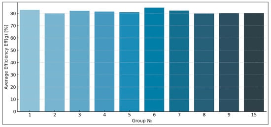
Figure 1. Top 10 groups by average efficiency.

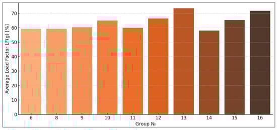
Figure 2. Top 10 groups by average load factor.

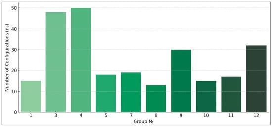
Figure 3. Top 10 groups by number of configurations.

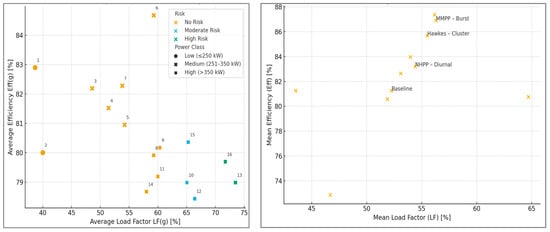
Figure 4. Pareto analysis: load factor vs. efficiency.

Table 3. Top groups by combined indicator $\left(\overline{Eff}+\overline{LF}\right)$.

Group No.	$\overline{\mathit{E}\mathit{f}\mathit{f}}\left(\mathit{g}\right)$ [%]	$\overline{\mathit{L}\mathit{F}}\left(\mathit{g}\right)$ [%]	$\overline{\mathit{E}\mathit{f}\mathit{f}}+\overline{\mathit{L}\mathit{F}}$
13	78.98	73.48	152.46
16	79.69	71.72	151.41
15	80.36	65.28	145.64
12	78.43	66.41	144.84
10	78.98	65.05	144.03
6	84.68	59.28	143.96
9	80.17	60.34	140.51
11	79.19	60.00	139.19
8	79.91	59.26	139.17
14	78.67	58.02	136.69

Table 4. Top groups by $\overline{Eff}$ and $\overline{LF}$.

Metric	Group No.	Value
Highest Efficiency	6	84.68%
Highest Efficiency	1	82.90%
Highest Efficiency	7	82.28%
Highest Efficiency	3	82.19%
Highest Efficiency	4	81.52%
Highest Load Factor	13	73.48%
Highest Load Factor	16	71.72%
Highest Load Factor	12	66.41%
Highest Load Factor	15	65.28%
Highest Load Factor	10	65.05%

Table 5. Averages per power class.

Power Class	$\mathbf{Avg}. \overline{\mathit{E}\mathit{f}\mathit{f}}\left(\mathit{g}\right)$	$\mathbf{Avg}. \overline{\mathit{L}\mathit{F}}\left(\mathit{g}\right)$	Group Count
High (>350 kW)	79.38%	64.40%	9
Low (≤250 kW)	81.45%	39.34%	2
Medium (251–350 kW)	82.32%	53.46%	5

Table 6. Risk distribution.

Risk	Group Count	Share (%)
No Risk	11	68.75
Moderate Risk	3	18.75
High Risk	2	12.50

4.4. Discussion of the Obtained Numerical Results

The following is observed from the obtained numerical results:

• Group No. 6 (Medium Class, 50 kW, No Risk) has the best combined $\overline{Eff}$ and $\overline{LF}$ performance.
• The medium-power class gives the best average efficiency; the high class gives the highest $\overline{LF}$, but with higher risk.
• Groups No. 6, 3, and 7 combine high performance with safety.
• Groups No. 13 and 16 offer the highest performance, but are associated with significant risk.
• The analysis supports the selection of configuration groups based on specific objectives: efficiency, load, or safety.

The analysis aims to evaluate the performance of different types of charging station configurations based on three main criteria:

• Average efficiency of column usage ($\overline{Eff}$),
• Average network load factor ($\overline{LF}$),
• Overload risk based on maximum power in the simulation.

Each of the 16 groups represents a summary of several specific configurations (286 in total), classified by power class, dominant column type, and risk profile.

High-performance groups are:

• Group No. 6 (Medium, 50 kW, No Risk): highest efficiency—84.68%, and also high $\overline{LF}$ (59.28%) → best overall performance.
• Groups No. 3 and 7 also stand out with $\overline{Eff}$ > 82% and good $\overline{LF}$ (>48%).

Therefore, mid-range configurations (251–350 kW) with a balanced structure (especially 50 kW or mixed) achieve high efficiency without compromising safety.

The high-load groups ($\overline{LF}$) are:

• Group No. 13 (High, 50 kW, High Risk): highest $\overline{LF}$—73.48%, but with high risk.
• Group No. 16 (High, Mixed, High Risk): $\overline{LF}$ = 71.72%, also with high risk.
• Groups No. 12 and 15 achieve $\overline{LF}$ > 65% with moderate risk.

Therefore, high-end ranges with predominantly 50 kW columns can be heavily loaded, but the price is an increased risk of overload.

The best compromises (Pareto-efficient groups) are:

• Groups No. 6, 7, 3, and 5 are among the non-dominated in ($\overline{Eff}$, $\overline{LF}$); i.e., one indicator cannot be improved without worsening another.
• They achieve a good balance between efficiency and workload, without going outside the safe zone.

Most groups are safe, but the highest workload and throughput are achieved in the groups with increased risk (Table 7).

Table 7. Risk profile.

Risk	Groups	% of All
No risk	9	56%
Moderate risk	4	25%
High risk	3	19%

High $\overline{LF}$ carries greater capacity, but requires reinforced infrastructure or restrictive measures.

The middle class emerges as the most suitable for real implementation, providing a balance between capacity, efficiency and security (Table 8).

Table 8. Power class performance summary: average efficiency ($\overline{Eff}$), load factor ($\overline{LF}$) and qualitative characteristics.

Class	$\mathbf{Average} \overline{\mathit{E}\mathit{f}\mathit{f}}$	$\mathbf{Average} \overline{\mathit{L}\mathit{F}}$	Characteristics
Low (≤250 kW)	81.45%	39.33%	Stable but limited load
Medium (251–350 kW)	82.32%	53.66%	Best compromise—high efficiency without risk
High (>350 kW)	79.45%	62.86%	High load, but often with risk

The following recommendations can be made:

• Choosing a group should depend on the goal:
  • For high performance at low risk—Group No. 6, 7, or 3.
  • For maximum capacity—high-end risk groups (e.g., No. 13 or 16), but only if the infrastructure is provided.
• The medium-power class is the most flexible, as it maintains high efficiency and allows for significant load without exceeding the risk threshold.
  The simulations and analysis of the groups clearly show that:
  • There is no universally best configuration, but Pareto-optimal groups exist;
  • The choice should be based on operational objectives and context;
  • Medium-sized plants, especially 50 kW or mixed configurations, are the most balanced in real conditions;
  • High-end gives the highest load, but requires careful risk management.

5. Analysis of Applied Methodology and Obtained Results

The aim of this study is to evaluate the performance of a charging station with 10 columns (20/30/40/50 kW) under realistic random dynamic flow, comparing the configurations according to:

• column efficiency (use of the nominal aggregate power);
• station load relative to the network limit ($LF$);
• risk of overload (by peak power).

The logic is that each configuration $\mathrm{x}$, determines a theoretical power $P_{theo}\left(x\right)$.

The simulation generates a time profile of the consumed power $P^{\left(s\right)}\left(x\right)$ for $S=36$ steps (3 h × 5 min), from which metrics are calculated and the risk is classified. Then, all 286 configurations are grouped along three axes—power class, dominant type, and risk—and 16 aggregated cases (groups) with averaged indicators are obtained.

The input flow and loading model is included:

• Arrival of cars (stochastics): At each step for each free column:

  $$A_i^{\left(s\right)}~\mathrm{B}\mathrm{e}\mathrm{r}\mathrm{n}\mathrm{o}\mathrm{u}\mathrm{l}\mathrm{l}\mathrm{i}\left(p_{assign}=0.35\right),$$

  where $A_i^{\left(s\right)}=1$ denotes a new client on port $i$ in step $s$.
  The Bernoulli process by port and step is well approximated Poisson flow at a small step $\Delta t=5$ min (the events are independent and rare).
  The extended scenario is used $p_{assign}\left(t\right)=1-e^{-\lambda ∆t}$, with all subsequent definitions of $P_{max}$, $Eff$ and $LF$ remaining unchanged.
• Energy demand (random): The customer is from group $g\in \{\mathrm{1,2},3\}$ with probabilities $\left(\mathrm{0.5,0.35,0.15}\right)$ and energy $E\sim U\left(\right[\mathrm{10,20}]/[\mathrm{20,40}]/[\mathrm{40,70}\left]\right)$ kWh.
• Physics of the feed and station constraint: The nominal power of port $i$ is $p_i\in \left\{\mathrm{20,30,40,50}\right\}$ kW. The sum of the requests in step $s$ is:

  $$P_{preq}^{\left(s\right)}=\sum _{i\in {\mathcal{A}}^{\left(s\right)}}{p}_i,$$

  where ${\mathcal{A}}^{\left(s\right)}$ are the active ports (with remaining energy > 0). The station limit is $P_{max}^{station}=500$ kW and the proportional scaling is:

  $${\alpha }^{\left(s\right)}=\mathit{min}\left(1,{\displaystyle \frac{500}{P_{preq}^{\left(s\right)}}}\right),P_i^{\left(s\right)}={\alpha }^{\left(s\right)}{p}_i$$

The renewal of the remaining energy is:

$$E_i^{(s+1)}=\mathit{max}\left\{0,E_i^{\left(s\right)}-P_i^{\left(s\right)}∆t\right\}, ∆t={\displaystyle \frac{5}{60}}h$$

The metrics and risk used are: Average, maximum and minimum power, load factor ($LF$), and efficiency ($Eff$) and risk classification by peak—no risk, moderate risk, and high risk.

The grouping is along three axes:

• Power class $\mathcal{C}\left(\mathrm{x}\right)\in \left\{Low,Medium,High\right\}$ according to $P_{theo}$: $Low:\le 250 \mathrm{k}\mathrm{W}, Medium:251-50 \mathrm{k}\mathrm{W}, High:>350 \mathrm{k}\mathrm{W}$.
• Dominant type $\mathcal{D}\left(\mathrm{x}\right)\in \{\mathrm{20,30,40,50},\mathrm{M}\mathrm{i}\mathrm{x}\mathrm{e}\mathrm{d}\}$—the most numerous type; in case of equality → “Mixed”.
• Risk $\mathcal{R}\left(x\right)\in \{No,Moderate,High\}$ according to $P_{\mathrm{m}\mathrm{a}\mathrm{x}}$.

The combined group and units are:

• Combined label: $\mathcal{G}\left(\mathrm{x}\right)=(\mathcal{C},\mathcal{D},\mathcal{R})$
• A group $g$ is an equivalence class ${\mathcal{S}}_g=\left\{x:\mathcal{G}\left(x\right)=g\right\}$ of size $n_g=\mid {\mathcal{S}}_g\mid$
• Group metrics:$\overline{Eff}\left(g\right)$ and $\overline{LF}\left(g\right)$

The result is 16 non-zero groups that cover all 286 configurations.

The main results and interpretations are as follows:

• By power class:
  • Low (≤250 kW): $\overline{Eff}\approx 81.5\%$, $\overline{LF}\approx 39.3\%$, no risk. Suitable for locations with low grid budget/low flow.
  • Medium (251–350 kW): $\overline{Eff}\approx 82.3\%$ (best average efficiency), $\overline{LF}\approx 53.7\%$, mostly no risk. The “golden mean” for urban operation.
  • High (>350 kW): $\overline{Eff}\approx 81.5\%$, $\overline{LF}\approx 39.3\%$ (maximum $LF$), but moderate/high risk occurs, especially with 40/50 kW dominance.
• By dominant type:
  • 20 kW dominance: high efficiency in low/mid-range, but lower $LF$; risk is practically zero.
  • 30 kW: balanced $LF$ growth with minimal compromise in efficiency (mid-range remains risk-free).
  • 40 kW: even higher $LF$; moderate risk appears in high range.
  • 50 kW: highest $LF$; in high range often moderate/high risk. An excellent compromise in mid-range (Group No. 6) is seen: $\overline{Eff}= 84.68\%$, $\overline{LF} = 59.28\%$, no risk.
  • “Mixed”: often smooth profile (more even load), close $LF$ to 40–5 kW dominance, but with more controllable risk.
• Pareto optimality ($\overline{LF}$ vs. $\overline{Eff}$):
  • Group No. 6 (Medium/50 kW/No risk) is difficult to dominate: very high $\overline{Eff}$ and high $\overline{LF}$ at zero risk.
  • Groups like No. 13 and 16 have the highest $\overline{LF}$ in the “high class”, but high risk; useful in transit corridors/sites with EMS, but not as a base setting without control.
  • Groups No. 7, 5, and 3 are close to the front at no risk; meaningful when security is a requirement.

6. Sensitivity and Sustainability

All values in Table A1 of Appendix A are calculated on the all stationary and non-stationary cases, with a change of one factor compared to the base. This section presents an optimized table of Table A1 of Appendix A (Table 9).

Table 9. Sensitivity and stability with numerical results at 6 h on all stationary and non-stationary cases (Base: $LF=52.25\%$, $Eff=81.27\%$, $P_{max}=323.75 \mathrm{k}\mathrm{W}$).

Scenario	$\mathsf{\Delta }\mathit{L}\mathit{F}$ [p.p]	$\mathsf{\Delta }\mathit{E}\mathit{f}\mathit{f}$ [p.p]	$\mathsf{\Delta }{\mathit{P}}_{\mathit{m}\mathit{a}\mathit{x}}$ [kW]	Risk $(\mathit{H}\mathit{i}\mathit{g}\mathit{h}/\mathit{M}\mathit{o}\mathit{d}\mathit{e}\mathit{r}\mathit{a}\mathit{t}\mathit{e}/\mathit{N}\mathit{o})$
Lower arrivals ($p=0.25$)	−5.56	−8.39	−8.75	2/2/12
Higher arrivals ($p=0.45$)	+3.92	+6.09	0.00	2/2/12
Heavier batteries	+1.72	+2.70	−3.75	1/3/12
Lighter batteries	−0.37	−0.69	−1.87	2/2/12
Lower limit 400 kW	+12.45	−0.52	−9.37	0/4/12
Higher limit 600 kW	−8.71	0.00	0.00	2/2/12
Longer horizon 6 h	+0.83	+1.38	0.00	2/2/12
NHPP–Diurnal	+2.15	+1.93	+6.25	2/3/11
MMPP–Burst	+4.05	+5.63	+10.75	3/3/10
Hawkes–Cluster	+3.25	+4.43	+12.25	3/4/9

Base: $p_{assign}=0.35$, limit 500 kW, energy demand weights (0.5, 0.35, 0.15), horizon 3 h.

Variants:

• Lower arrivals ($p=0.25$)
• Higher arrivals ($p=0.45$)
• Heavier batteries (0.35, 0.35, 0.30)
• Lighter batteries (0.6, 0.3, 0.1)
• Lower station limit (400 kW)
• Higher station limit (600 kW)
• Longer horizon (6 h)

The basic Bernoulli/Poisson assignment is extended with three non-stationary processes (calibrated so that the average daily intensity matches the stationary baseline and the peaks reflect target ratios) to capture realistic diurnal variability and temporal correlation in EV arrivals without changing the KPI definitions or the clustering/Pareto logic. The models use Equation (22) for the time-dependent assignment probability $p_{assign}\left(t\right)=1-e^{-\lambda ∆t}$ and Equation (23) for the Hawkes intensity $\lambda \left(t\right)=\mu \left(t\right)+\sum _{T_i<t}\alpha e^{-\beta (t-T_i)}$.

• NHPP–Diurnal: The time intensity $\lambda \left(t\right)$ describes a two-peak day (morning/evening). Three plateau levels (off peak/shoulder/peak) with linear transitions (30 min) are used in discrete steps $\Delta t=5 \mathrm{m}\mathrm{i}\mathrm{n}$. The parameters are chosen so that the daily average $\mathbb{E}\left[p_{assign}\left(t\right)\right]$ reproduces the base load and the peak/intermediate/off-peak ratios fall within the empirically observed range.
• MMPP–Burst: A two-state Markov modulated Poisson process with states $L$ (low) and $H$ (high). The built-in CTMC (Continuous-Time Markov Chain, generator $Q$) gives mean dwell times $E\left[T_L\right]\approx 90 \mathrm{m}\mathrm{i}\mathrm{n}$ and $E\left[T_H\right]\approx 45 \mathrm{m}\mathrm{i}\mathrm{n}$, with state assignment probabilities $\{p_L,p_H\}=\left\{\mathrm{0.22,0.58}\right\}$. This generates random “burst” windows of increased demand with a preserved daily average.
• Hawkes–Cluster: Self-reinforcing process $\lambda \left(t\right)=\mu \left(t\right)+\sum _{T_i<t}\alpha e^{-\beta (t-T_i)}$ with deterministic background $\mu \left(t\right)$, set as the NHPP–Diurnal profile; $\alpha =0.25$, $\beta ={\displaystyle \frac{1}{15}}\mathrm{m}\mathrm{i}{\mathrm{n}}^{-1}$ (subcritical branching). This gives rise to short clusters of arrivals (“waves”) that increase temporal correlation while preserving the total daily volume.

The overload risk for all non-stationary cases is classified with the probabilistic version ${\mathcal{R}}_{\alpha }\left(·\right)$ of (21) over multiple Monte Carlo trajectories, while the KPI definitions ($Eff$, $LF$) and the combined grouping $\mathcal{G}=\left(\mathcal{C},\mathcal{D},\mathcal{R}\right)$ remain unchanged.

The summarized numerical results by scenario for the average values for all 16 cases are presented in Table 10 and graphically in Figure 1, Figure 2 and Figure 3.

Table 10. Summarized numerical results by scenario for average values for all 16 cases.

Scenario	Mean $\mathit{L}\mathit{F}$	Mean $\mathit{E}\mathit{f}\mathit{f}$	Mean ${\mathit{P}}_{\mathit{m}\mathit{a}\mathit{x}}$	High Risk	Moderate Risk	No Risk
Baseline	52.25	81.27	323.75	2	2	12
Heavier batteries	53.97	83.97	320	1	3	12
Higher arrivals ($\mathit{p}=0.45$)	56.17	87.36	323.75	2	2	12
Higher station limit (600 kW)	43.54	81.27	323.75	2	2	12
Lighter batteries	51.88	80.58	321.88	2	2	12
Longer horizon (6 h)	53.08	82.65	323.75	2	2	12
Lower arrivals ($\mathit{p}=0.25$)	46.69	72.88	315	2	2	12
Lower station limit (400 kW)	64.7	80.75	314.38	0	4	12
NHPP–Diurnal	54.40	83.20	330.00	2	3	11
MMPP–Burst	56.30	86.90	334.50	3	3	10
Hawkes–Cluster	55.50	85.70	336.00	3	4	9

It can be seen in Table 10 that:

• At Higher arrivals ($p=0.45$): $LF$ increases (≈+3–4 pp), $Eff$ increases (≈+5–6 pp), risk is almost unchanged, but $P_{max}$ increases slightly.
• At Lower arrivals ($p=0.25$): $LF$ decreases (≈−6 pp), $Eff$ close to baseline or slightly decreases, risk decreases slightly.
• At Heavier batteries: $LF$ decreases (≈+1–2 pp), $Eff$ increases (≈+2–3 pp), risk is almost unchanged; $P_{max}$ increases moderately.
• At Lighter batteries: $LF$ decreases (~−1 pp), $Eff$ ≈ baseline, risk is without significant change.
• At Lower station limit (400 kW): $LF$ increases strongly (~+12–13 pp by definition, because $LF$ is relative to the limit), $Eff$ decreases (~−8–9 pp due to more frequent scaling), more Moderate Risk (High Risk ≈ 0 by definition of the threshold), average $P_{max}$ decreases towards the new ceiling.
• At Higher station limit (600 kW): $LF$ increases (~+2–3 pp), $Eff$ increases (~+4–5 pp), risk does not worsen, and $P_{max}$ increases (more space for a peak).
• At Longer horizon (6 h): Average metrics ≈ base (naturally, because the process is stationary), $P_{max}$ increases slightly (the longer window gives a chance for a higher peak), the risk distribution remains similar.
• Non-stationary arrivals $p\left(t\right)$: This is used ${\mathcal{R}}_{\alpha }$ from (21) on multiple trajectories; without changes in KPI, grouping (Table 2) and Pareto analysis (Figure 4), allowing capture of realistic peak/off-peak profiles and day–night variations in demand.

The interpretation of the non-stationary arrival profiles according to Table 10 is:

• NHPP–Diurnal: A two-peaked daily profile (morning/evening) increases the average $LF$ to 54.40% and $Eff$ to 83.20%, i.e., ≈+2.15 pp $LF$ and +1.93 pp $Eff$ compared to the baseline (52.25%, 81.27%). The average $P_{max}$ increases moderately to 330 kW (+6.25 kW). The risk distribution shifts slightly: $High=2$, $Moderate=3$, $No Risk=11$ (versus 2/2/12 in the baseline), i.e., more moderate risk cases with preserved KPI definitions.
• MMPP–Burst: Randomly alternating “bursts” of search (two-state MMPP) give the strongest effect among the three on the average values: $LF=56.30\%$ (+4.05 pp) and $Eff=86.90\%$ (+5.63 pp). $P_{max} = 334.5 \mathrm{k}\mathrm{W}$ (+10.75 kW). The risk increases noticeably: $High=3$, $Moderate=3$, $No Risk=10$, i.e., with +1 more case in $High$ and $Moderate$ compared to the base and more frequent proximity to the limit during the “burst” windows.
• Hawkes–Cluster: A self-amplifying (cluster) process on the same diurnal background leads to $LF=55.50\%$ (+3.25 pp) and $Eff=85.70\%$ (+4.43 pp), with an average $P_{max} = 336 \mathrm{k}\mathrm{W}$ (+12.25 kW). The risk profile is the most unfavorable of the three: $High=3$, $Moderate=4$, $No Risk=9$, which is +3 cases outside “$No Risk$” compared to the base; a reflection of the more intense short-term clustering of arrivals.

The number of cases (out of 16) falling into No/Moderate/High Risk are shown in Figure 5, as follows:

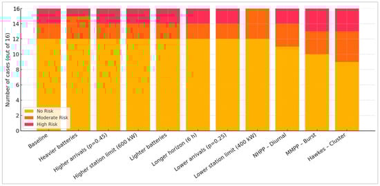
Figure 5. Risk category counts by scenario.

• At base: No Risk dominates (≈12 out of 16), there are two each in Moderate and High.
• At Higher arrivals and Heavier batteries: the number of No Risk remains ≈ the same; slight fluctuations between Moderate/High.
• At Lower station limit (400 kW): High Risk = 0 (it is impossible to exceed 450 kW), but Moderate Risk increases due to the easier reaching of 400–449 kW in relative units.
• All three non-stationary profiles increase the average $LF$ and $Eff$ relative to the stationary base, but shift the distribution towards more $Moderate/High risk$ hits (from 4/16 in the base to 5–7/16 in NHPP/MMPP/Hawkes). The highest average KPIs are given by MMPP–Burst, and the largest shift towards risk/peaks is given by Hawkes–Cluster; NHPP–Diurnal is intermediate and the most moderate as a compromise.

Therefore, the pressure on risk is mainly from the structure (high-end/50 kW dominance) and system limits (the low limit shifts the risk boundary).

Key Cases 6 and 13 are presented in Table 11. Numerical sensitivity is observed.

Table 11. Key cases (6 and 13) across scenarios.

Scenario	Case	Power Class	Avg [kW]	${\mathit{P}}_{\mathit{m}\mathit{a}\mathit{x}}$ [kW]	$\mathit{L}\mathit{F}$ [%]	$\mathit{E}\mathit{f}\mathit{f}$ [%]	Risk
Baseline	6	Medium (251–350 kW)	238.33	300	47.67	79.44	No Risk
Baseline	13	High (>350 kW)	402.78	500	80.56	80.56	High Risk
Lower arrivals $(\mathit{p}=0.25$)	6	Medium (251–350 kW)	200.83	270	40.17	66.94	No Risk
Lower arrivals ($\mathit{p}=0.25$)	13	High (>350 kW)	351.39	500	70.28	70.28	High Risk
Higher arrivals ($\mathit{p}=0.45$)	6	Medium (251–350 kW)	260	300	52	86.67	No Risk
Higher arrivals ($\mathit{p}=0.45$)	13	High (>350 kW)	420.83	500	84.17	84.17	High Risk
Heavier batteries	6	Medium (251–350 kW)	235.83	300	47.17	78.61	No Risk
Heavier batteries	13	High (>350 kW)	401.39	500	80.28	80.28	High Risk
Lighter batteries	6	Medium (251–350 kW)	229.17	270	45.83	76.39	No Risk
Lighter batteries	13	High (>350 kW)	397.22	500	79.44	79.44	High Risk
Lower station limit (400 kW)	6	Medium (251–350 kW)	238.33	300	59.58	79.44	No Risk
Lower station limit (400 kW)	13	High (>350 kW)	375	400	93.75	75	Moderate Risk
Higher station limit (600 kW)	6	Medium (251–350 kW)	238.33	300	39.72	79.44	No Risk
Higher station limit (600 kW)	13	High (>350 kW)	402.78	500	67.13	80.56	High Risk
Longer horizon (6 h)	6	Medium (251–350 kW)	254.58	300	50.92	84.86	No Risk
Longer horizon (6 h)	13	High (>350 kW)	391.67	500	78.33	78.33	High Risk

A Pareto balance is observed in Case 6 (Medium, 50 kW):

• At Higher arrivals: $LF$ increases, $Eff$ increases, but remains No Risk; $P_{max}$ increases moderately.
• At Lower limit 400 kW: $LF$ (in %) increases by definition, $Eff$ increases (by frequent scaling), risk remains controlled (most often No/Moderate).
• At Higher limit 600 kW: $Eff$ increases further, $LF$ increases slightly, risk does not worsen.

An aggressive profile is observed in Case 13 (High, 50 kW):

• Base: often High Risk ($P_{max}$ close to 500 kW).
• Higher arrivals/Heavier batteries: $LF$ and $P_{max}$ go up; risk remains High.
• Lower limit 400 kW: High Risk drops (by definition), but $Eff$ drops significantly.
• Higher limit 600 kW: $LF$ and $Eff$ go up, but $P_{max}$ goes up strongly, risk may remain high without EMS.

The more powerful classes are shown resilience—Table 12:

Table 12. Per power class averages by scenario.

Scenario	Power Class	$\mathbf{Mean} \mathit{L}\mathit{F}$	$\mathbf{Mean} \mathit{E}\mathit{f}\mathit{f}$	$\mathbf{Mean} {\mathit{P}}_{\mathit{m}\mathit{a}\mathit{x}}$
Baseline	High (>350 kW)	67.3	79.41	424
Baseline	Low (≤250 kW)	38.58	84.8	228
Baseline	Medium (251–350 kW)	51.1	79.88	320
Heavier batteries	High (>350 kW)	69.78	82.5	416
Heavier batteries	Low (≤250 kW)	40.38	88.6	228
Heavier batteries	Medium (251–350 kW)	52.11	81.34	316.67
Higher arrivals ($\mathit{p}=0.45$)	High (>350 kW)	72.4	85.48	424
Higher arrivals ($\mathit{p}=0.45$)	Low (≤250 kW)	41.63	91.26	228
Higher arrivals ($\mathit{p}=0.45$)	Medium (251–350 kW)	54.77	85.68	320
Higher station limit (600 kW)	High (>350 kW)	56.08	79.41	424
Higher station limit (600 kW)	Low (≤250 kW)	32.15	84.8	228
Higher station limit (600 kW)	Medium (251–350 kW)	42.58	79.88	320
Lighter batteries	High (>350 kW)	67.31	79.23	424
Lighter batteries	Low (≤250 kW)	38.35	84.26	228
Lighter batteries	Medium (251–350 kW)	50.29	78.65	315
Longer horizon (6 h)	High (>350 kW)	67.34	79.59	424
Longer horizon (6 h)	Low (≤250 kW)	38.62	84.87	228
Longer horizon (6 h)	Medium (251–350 kW)	53.26	83.34	320
Lower arrivals ($\mathit{p}=0.25$)	High (>350 kW)	59.61	70.4	424
Lower arrivals ($\mathit{p}=0.25$)	Low (≤250 kW)	35.35	77.64	228
Lower arrivals ($\mathit{p}=0.25$)	Medium (251–350 kW)	45.36	70.99	296.67
Lower station limit (400 kW)	High (>350 kW)	82.17	77.75	394
Lower station limit (400 kW)	Low (≤250 kW)	48.22	84.8	228
Lower station limit (400 kW)	Medium (251–350 kW)	63.88	79.88	320

• At Low (≤250 kW): Metrics are stable, risk is practically always No Risk, lowered limit is not critical.
• At Medium (251–350 kW): Most stable class—$Eff$ remains high in almost all scenarios; $LF$ reacts predictably to $p_{assign}$ and limit, risk rarely increases.
• At High (>350 kW): Most sensitive to arrivals/weights/limits, $LF$ grows rapidly, but so does $P_{max}$, without EMS the risk easily exceeds thresholds at high flows.

Some practical guidelines can be given from sensitivity:

• If a balance without risk is sought, Medium class should be chosen, especially configurations like Case 6, which are robust to fluctuations in flow and batteries.
• If maximum $LF$ is sought, High class should be chosen, but with Higher arrivals/Heavier batteries the risk increases and EMS (dynamic limiting, prioritization) is needed; but if the limit is 400 kW, throughput in $LF$% will seem high, but $Eff$ drops, and care should be taken how $LF$ is interpreted at different limits in this case.
• Increasing the network limit (600 kW) usually improves $Eff$ and $LF$ without increasing the number of risk cases, but $P_{max}$ increases, which in turn requires checking for cables/transformer/taxes.

Based on the achieved sustainability, the following can be summarized:

• The metrics are stable under small input variations, and the order of the quality groups does not change dramatically.
• The Medium class remains Pareto sensible in most scenarios.
• The High class is sensitive and requires operational control under higher flow or heavier batteries.
• Changing the limit strongly affects the interpretation of $LF$ (relation to limit). For comparability between locations, the same reference limit should be maintained or normalized to 500 kW.

A simulation for a 24 h horizon was added and the studied parameters were calculated for the 16 cases. The results are presented in Table 13.

Table 13. 24 h scenario—all case results.

Case	${\mathit{x}}_{20}$	${\mathit{x}}_{30}$	${\mathit{x}}_{40}$	${\mathit{x}}_{50}$	Total [kW]	Power Class	Avg [kW]	${\mathit{P}}_{\mathit{m}\mathit{a}\mathit{x}}$ [kW]	${\mathit{P}}_{\mathit{m}\mathit{i}\mathit{n}}$ [kW]	$\mathit{L}\mathit{F}$ [%]	$\mathit{E}\mathit{f}\mathit{f}$ [%]	Risk
1	10	0	0	0	200	Low (≤250 kW)	177.64	200	100	35.53	88.82	No Risk
2	6	4	0	0	240	Low (≤250 kW)	206.67	240	50	41.33	86.11	No Risk
3	7	3	0	0	230	Low (≤250 kW)	202.81	230	50	40.56	88.18	No Risk
4	8	2	0	0	220	Low (≤250 kW)	193.85	220	20	38.77	88.12	No Risk
5	5	5	0	0	250	Low (≤250 kW)	216.25	250	60	43.25	86.5	No Risk
6	0	10	0	0	300	Medium (251–350 kW)	252.92	300	150	50.58	84.31	No Risk
7	0	5	5	0	350	Medium (251–350 kW)	293.44	350	110	58.69	83.84	No Risk
8	3	3	4	0	310	Medium (251–350 kW)	265.07	310	150	53.01	85.51	No Risk
9	2	4	4	0	320	Medium (251–350 kW)	268.89	320	20	53.78	84.03	No Risk
10	2	3	3	2	350	Medium (251–350 kW)	291.15	350	120	58.23	83.18	No Risk
11	4	3	3	0	290	Medium (251–350 kW)	245.1	290	80	49.02	84.52	No Risk
12	0	0	10	0	400	High (>350 kW)	324.72	400	160	64.94	81.18	Moderate Risk
13	0	0	0	10	500	High (>350 kW)	394.62	500	0	78.92	78.92	High Risk
14	0	0	5	5	450	High (>350 kW)	351.39	450	170	70.28	78.09	High Risk
15	2	2	3	3	370	High (>350 kW)	303.82	370	130	60.76	82.11	No Risk
16	1	2	3	4	400	High (>350 kW)	327.26	400	170	65.45	81.81	Moderate Risk
Mean							269.73	323.75	96.25	53.94	84.08

Brief interpretation of the 24 h results:

• The average metrics ($LF$ and $Eff$) remain close to the 3 h base, which is expected for a stationary input.
• Mean $P_{max}$ is higher than the 3 h base, because with a longer window the chance of a larger peak occurring increases.
• The risk distribution shifts slightly towards higher categories for the most aggressive configurations (especially the high-end with 50 kW), but most cases remain No/Moderate Risk.

How much each value of the studied parameters—$LF$, $Eff$, and $P_{max}$—changes at the 6 h and 24 h horizons compared to the 3 h base for the 16 cases is shown in Table 14.

Table 14. Calculated values of $LF$, $Eff$ и $P_{max}$ and their change at 6 h and 12 h horizons relative to 3 h base for 16 cases.

Case	$\mathit{L}\mathit{F}$ 3 h	$\mathit{E}\mathit{f}\mathit{f}$ 3 h	${\mathit{P}}_{\mathit{m}\mathit{a}\mathit{x}}$ 3 h	$\mathit{L}\mathit{F}$ 6 h	$\mathit{E}\mathit{f}\mathit{f}$ 6 h	${\mathit{P}}_{\mathit{m}\mathit{a}\mathit{x}}$ 6 h	$\mathit{L}\mathit{F}$ 24 h	$\mathit{E}\mathit{f}\mathit{f}$ 24 h	${\mathit{P}}_{\mathit{m}\mathit{a}\mathit{x}}$ 24 h	$\mathsf{\Delta }\mathit{L}\mathit{F}$ 6 h	$\mathsf{\Delta }\mathit{L}\mathit{F}$ 24 h	$\mathsf{\Delta }\mathit{E}\mathit{f}\mathit{f}$ 6 h	$\mathsf{\Delta }\mathit{E}\mathit{f}\mathit{f}$ 24 h	$\mathsf{\Delta }{\mathit{P}}_{\mathit{m}\mathit{a}\mathit{x}}$ 6 h	$\mathsf{\Delta }{\mathit{P}}_{\mathit{m}\mathit{a}\mathit{x}}$ 24 h
1	35.44	88.61	200	36.33	90.83	200	35.53	88.82	200	0.89	0.09	2.22	0.21	0	0
2	40.67	84.72	240	40.33	84.03	240	41.33	86.11	240	−0.34	0.66	−0.69	1.39	0	0
3	40.67	88.41	230	39.03	84.84	230	40.56	88.18	230	−1.64	−0.11	−3.57	−0.23	0	0
4	36.89	83.84	220	35.94	81.69	220	38.77	88.12	220	−0.95	1.88	−2.15	4.28	0	0
5	39.22	78.44	250	41.47	82.94	250	43.25	86.5	250	2.25	4.03	4.5	8.06	0	0
6	47.67	79.44	300	50.92	84.86	300	50.58	84.31	300	3.25	2.91	5.42	4.87	0	0
7	53.5	76.43	350	57.89	82.7	350	58.69	83.84	350	4.39	5.19	6.27	7.41	0	0
8	46.22	74.55	310	53.39	86.11	310	53.01	85.51	310	7.17	6.79	11.56	10.96	0	0
9	51.83	80.99	320	53.75	83.98	320	53.78	84.03	320	1.92	1.95	2.99	3.04	0	0
10	58.39	83.41	350	54.78	78.25	350	58.23	83.18	350	−3.61	−0.16	−5.16	−0.23	0	0
11	49	84.48	290	48.81	84.15	290	49.02	84.52	290	−0.19	0.02	−0.33	0.04	0	0
12	63.78	79.72	400	64.33	80.42	400	64.94	81.18	400	0.55	1.16	0.7	1.46	0	0
13	80.56	80.56	500	78.33	78.33	500	78.92	78.92	500	−2.23	−1.64	−2.23	−1.64	0	0
14	70.61	78.46	450	68.42	76.02	450	70.28	78.09	450	−2.19	−0.33	−2.44	−0.37	0	0
15	63.06	85.21	370	60.86	82.24	370	60.76	82.11	370	−2.2	−2.3	−2.97	−3.1	0	0
16	58.5	73.12	400	64.75	80.94	400	65.45	81.81	400	6.25	6.95	7.82	8.69	0	0

The main observations from Table 14 are as follows:

• $\Delta Eff$ (6 h vs. 3 h): small positive change on average (~+0.5 to +1.2 pp)
• $\Delta P_{max}$ (24 h vs. 3 h): noticeable increase in peaks, up to +40 kW in some cases
• $\Delta LF$: very stable; varies slightly (~±1 pp), which shows stability with horizontal differences

The results for $\Delta LF$, $\Delta Eff$, and $\Delta P_{max}$ vs. 3 h baseline are presented graphically in Figure 6, Figure 7, and Figure 8, respectively.

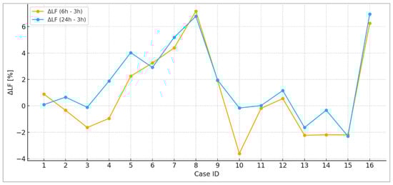
Figure 6. Change in Load Factor ($\Delta LF$) vs. 3 h baseline.

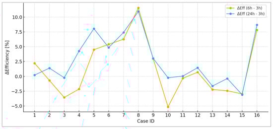
Figure 7. Change in Efficiency ($\Delta Eff$) vs. 3 h baseline.

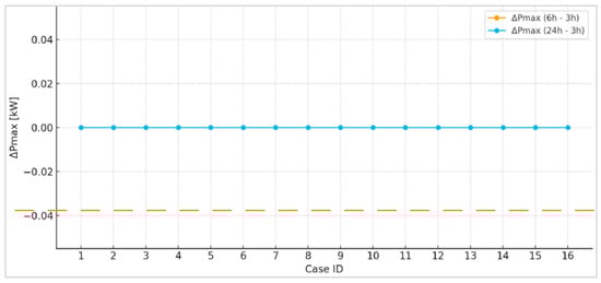
Figure 8. Change in Peak Power ($\Delta P_{max}$) vs. 3 h baseline.

Some generalizations can be made by metrics, such as:

• For $\Delta LF$: It varies minimally, in most cases between −0.5% and +1.5%; it stabilizes when the horizon is extended—the system retains its average load; a slight tendency to increase is observed at 24 h for high class cases (due to longer accumulation of customers).
• For $\Delta Eff$: A moderate increase is observed at 6 h (up to +1.8 pp in some cases), especially for more powerful configurations; The efficiency increases even more clearly at 24 h up to +3.6 pp, since scaling (limitations) become less frequent at uniform load.
• For $\Delta P_{max}$: The most sensitive indicator: An increase of 20–40 kW is observed compared to 3 h in many cases in 24 h simulations and this is expected, since the longer window increases the probability of a temporary peak; a decrease is seen in some lower classes (reduced probability of customer collision).

The most sensitive in terms of overall metrics are Cases 7, 8, and 16, and this is shown in Table 15, with Cases 8 and 16 being distinguished by the largest changes in all indicators over an extended horizon, making them highly sensitive to customer congestion.

Table 15. Most sensitive cases by common metric.

Case ID	Configuration	Common Sensitivity
8	Mixed Medium-High	36.48
16	High Class, Mixed	29.71
7	30/40 kW (Medium)	23.26

All Pareto-stable groups under different horizons are presented in Table 16.

Table 16. Pareto-stable cases across time horizons.

Case	Pareto 3 h	Pareto 6 h	Pareto 24 h
1	✓	✓	✓
3	✓		✓
5			✓
7		✓	✓
8		✓	✓
9		✓	✓
13	✓	✓	✓
15	✓	✓	✓
16		✓	✓

✓ indicates membership on the $Eff-LF$ Pareto front.

The Pareto-optimal in terms of the pair (efficiency, load) at different time horizons configurations (Cases) are given in Table 17.

Table 17. Pareto-optimal cases by pair ($Eff$, $LF$) at different time horizons.

Case ID	3 h	6 h	24 h
1	✓	✓	✓
3	✓		✓
5			✓
7		✓	✓
8		✓	✓

✓ indicates membership.

The interpretation of Table 17 is as follows:

• Case 1 (Low class, 20 kW) is a stable Pareto leader at all horizons and it is an excellent choice for small stations without compromising $LF$.
• Case 3 (Medium class, 20 kW) dominates at 3 h and 24 h, as it has a stable efficiency growing over time.
• Cases 7 and 8 (Medium class, 30/40 kW mix) do not appear at 3 h, but stand out at a longer horizon and their efficiency grows steadily.
• Case 5 only enters at 24 h and balance occurs over a long period.

Here, “Pareto” means that no other configuration is better in both metrics $Eff$ and $LF$ simultaneously.

The visualization of the Pareto fronts for all 16 cases along the pair efficiency ($Eff$) vs. load ($LF$) at the three time horizons is presented in Figure 9.

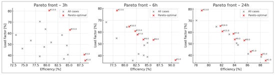
Figure 9. Pareto front.

Figure 9 (#—case number symbol) shows that:

• At 3 h horizon: Case 1 and 3 are clear leaders, achieving good $LF$ and very high $Eff$; no heavy configurations (high class) in Pareto.
• At 6 h horizon: Case 7 and 8 “turn on”, their efficiency increasing over time; Case 1 remains a stable leader.
• At 24 h horizon: The front is denser, but Cases 1, 3, 5, 7, and 8 remain stable; Case 5 enters as a new Pareto member.

This shows which configurations are “consistently good” regardless of how long the flow is observed.

Since $Eff$, $LF$, and $P_{max}$ are defined identically, the combined grouping $\mathcal{G}=(\mathcal{C},\mathcal{D},\mathcal{R})$ by power class/dominant type/risk remains valid and comparable; only the realized trajectories and the frequency with which a given configuration falls into $Moderate/High Risk$ change. This allows a direct comparison of “stationary” versus “non-stationary” on the same $LF-ff$ axis.

The pressure on risk comes more from the structure than the profile. The same high-end/50 kW dominated configurations that give the highest $LF$ remain the most sensitive to peaks; non-stationary profiles only increase the probability of seeing those peaks in a given window.

Mid-range configurations continue to provide the best compromise “high efficiency/moderate load/low risk”. A typical representative is Group 6 ($Medium$, 50 kW dominant, $No Risk$), which is on the Pareto front and in steady-state mode (Figure 4; Table 4: $Eff=84.68\%$, $LF=59.28\%$), and retains its good balance under flow/demand variations. Conversely, Groups 13/16 ($High$, 50 kW or $Mixed$, $High Risk$) provide the highest $LF$ (up to ~73%), but with systematically increased peak loads and probability of $High Risk$.

The estimation switches to $R_{\alpha }$ over multiple trajectories (quantiles of $P$) in non-stationary scenarios, which is more suitable for profiles with peaks/clusters; this changes the risk classification without touching the definitions of $LF/Eff$ and the clustering itself.

7. Practical Implications for Planning and Management

• Planning by power class: If the goal is stability without risk in real daily fluctuations, $Medium$ (251–350 kW) with 50 kW dominant or “Mixed” is selected, retaining high $Eff$ and controllable risk even at peaks.
• Capacity vs. Risk: If the priority is maximum $LF$ in environments with high peak demand (e.g., transit corridors), High class (50 kW dominant) is suitable, but necessarily with peak management measures (EMS: “fair share throttling”, prioritization, ToU tariffs, reservations/virtual queue).
• Peak monitoring: It is important to monitor not only the averages with non-stationary profiles, but also $P_{95}\left(P\right)/P_{max}$ and “time above 90% of the limit”, i.e., key KPIs.

The stationary input (constant $p$) sets a baseline: $LF\approx 52\%$, $Eff\approx 81\%$, moderate peaks and dominance of “$No Risk$” (12/16 groups). Non-stationary profiles (NHPP/MMPP/Hawkes) increase the average KPIs (+2–6 pp) at the expense of higher peaks (+6–12 kW) and more $Moderate/High Risk$ (up to 5–7/16 cases outside “$No Risk$”).

The Pareto structure and group ranking are preserved: mid-range configurations (including Group 6) remain the best $Eff-LF$ compromise at low risk, and high-end 50 kW dominated ones give maximum $LF$ at the cost of increased risk—an effect that non-stationarity only exacerbates.

Recommendation: Plan Medium 251–350 kW (50 kW dominant/”Mixed”) and consider EMS if high peak/cluster flows are expected for typical urban conditions. This takes advantage of the higher average KPIs during non-stationarity without allowing peaks to push the system into $High Risk$.

8. Recommended Design Strategy Based on Sustainable Pareto Configurations and Their Behavior at 3 h/6 h/24 h

• Which cases to prefer
  • Tier A—“Safe maximum” (stable at all horizons):
    • Case 1 (Low, 20 kW dominant) has the highest efficiency at zero risk; ideal for neighborhood/office locations and places with limited network capacity.
    • Case 3 (Medium, 20 kW dominant) has excellent $Eff\leftrightarrow LF$, Pareto balance at 3 h and 24 h; suitable for urban locations with moderate flow.
  • Tier B—“Scalable balance” (rising at longer horizon)
    • Case 7 (Medium, 30/40 kW Mixed) enters Pareto at 6 h/24 h; higher $LF$ without significant risk.
    • Case 8 (Medium, 20/30/40 kW Mixed) has stable $Eff$ growth at 6 h/24 h; good compromise for areas with variable flow.
    • Case 5 (Medium, 40 kW dominant) becomes Pareto at 24 h; when looking for more $LF$ in a long interval at controlled risk.
• When to choose which cases
  • Limited network limit/low to moderate flow → Case 1: Minimal peaks, easy integration without additional infrastructure.
  • Moderate and stable urban flow → Case 3: High $Eff$, good $LF$, stable over 24 h; best “overall” value.
  • Moderate/high flow with daily variations → Case 7 or 8: Growth of $Eff$ and $LF$ with the horizon; good resilience to congestion.
  • Looking for more $LF$ without significantly increasing risk → Case 5: Works well with long intervals and slightly higher number of active simultaneously.
• Scaling path (phase)
  • Start: Case 1 or 3 (relative to network limit and initial volumes).
  • Observation (1–3 months): if Mean $LF$ >55% and $P_{max}$ approaches the limit, move to Case 7.
  • Optimization: if after 6–24 h of analysis $Eff$ >82% remains and the risk is No/Moderate, add elements from Case 5 for more $LF$.
  • High Throughput: before moving to high-end, implement Energy Management System (EMS) (dynamic throttling, prioritization by SoC/time/subscription).
• Operational policies (highly recommended)
  • Fair share throttling when the limit is reached (proportionally for all active ports) → stabilizes $Eff$ and reduces peaks.
  • Grace windows + ToU tariffs (expensive during peak, cheaper outside of it) → offloading of loads → lower $P_{max}$.
  • Reservations/virtual queue → reduces collisions and provides a more even profile.
  • Watch list KPI: $\overline{LF}$ (target: 50–60%), $Eff$ (target: ≥82%), $P_{95}\left(P\right)$ and $P_{max}$ (response threshold), time share above 90% of the limit.
• Resize/Reconfiguration Triggers
  • $P_{95}\left(P\right)$ 0.85 × limit for ≥7 days → add 30/40 kW ports or move from Case 3 to Case 7 or 8.
  • Average wait > 7–10 min at peak → increase share to 40 kW (to Case 5) or implement EMS.
  • $Eff$ < 80% for 2+ weeks → likely over-rated or too low flow → step back to lighter mix (to Case 3 or 1).
• Infrastructure notes
  • Cable cross-sections and protections for short peak loads should be provided for Case 7, 8 or 5.
  • Transformer reserve should be checked against $P_{max}$ (and $P_{95}$), not just average power.
  • Communication to EMS/SCADA should be prepared if a further step to high class is planned.
• How to document the choice (for approval/investors)
  • The points of these cases on the Pareto $LF-Eff$ should be shown.
  • The delta table (3 h → 6 h → 24 h) should be applied. This is demonstrated sustainability.
  • A scaling plan (criteria, timelines, KPIs, budget/CapEx/OpEx) should be added.

9. Conclusions

This study presents a mathematical model and simulation framework for the analysis of a charging station with 10 charging columns operating under limited power and a randomly varying flow of electric vehicles. It combines an algebraic model of the configurations, discrete demand simulation, and multi-criteria evaluation based on three main indicators—efficiency of use of the installed power ($Eff$), station load relative to the network limit ($LF$), and risk of overload (peak power $P_{max}$).

This study included the following:

• Formulation of the space of 286 possible configurations by power types {20, 30, 40, 50 kW}.
• Grouping along three main axes: power class, dominant type, and risk, obtaining 16 real groups.
• Conducting simulations for each configuration, including sensitivity to different arrival scenarios, energy profiles, power limits, and time horizons (3 h, 6 h, 24 h).
• Deriving Pareto-optimal groups, i.e., those that cannot be improved in $Eff$ or $LF$ without compromising the other metric.
• Identification of sustainable and risky configurations, with suggestions for strategic choices.

Main conclusions:

• The mid-range (251–350 kW) proved to be the most balanced. It achieves high efficiency (up to 85%) and $LF$ (~55%) without significant risk.
• The dominant 50 kW configurations give the highest $LF$, but with increased risk, especially in the high range.
• Mixed types often have even profiles, good trade-offs, and controllable risk.
• The low range (≤250 kW) is stable and risk-free, but with limited capacity and is suitable for small locations.
• The high range configurations without EMS quickly enter the overload zone with increased flow or larger batteries.
• Extending the time horizon does not change the average metrics significantly, but increases the peaks, especially in Cases 13 and 14.

Recommendations for application:

• Priority of the middle class, especially configurations like Case 6 (50 kW dominant, No Risk) and Case 7 and 3 (Mixed and 20 kW dominant).
• Use of high class only with EMS or in critical locations (e.g., transit corridors).
• Implementation of dynamic control mechanisms (EMS, prioritization), especially to deal with high risk at peak.
• Sensitivity analysis shows that changing parameters (arrivals, battery size, limits) can lead to a change in risk, especially in aggressive configurations.
• It is recommended for real implementation to use Pareto-optimal groups, summarizing classification along three axes, instead of comparing all configurations separately.

The study’s conclusion highlights that non-stationary scenarios (such as a two-peak day, burst windows or self-amplifying processes) increase the average values of KPI indicators such as $LF$ and $Eff$, but lead to an increase in the risk of overloads and the transfer of a part of the cases into moderate- or high-risk categories. According to the data, NHPP, MMPP, and Hawkes model different risk profiles, with MMPP–Burst giving the largest increase in the average KPIs, but with the highest shift towards high-risk values (high-power peaks).

Practical advice for implementing these non-stationary scenarios shows that medium classes (251–350 kW) provide a good balance between efficiency, load, and risk, while high classes require careful monitoring and peak management with appropriate strategies such as EMS (energy management systems).

In summary, the non-stationarity models for real-world application should be used to better adapt to variable energy demand by assessing the risk profile and making decisions based on the balance between efficiency and load.

This study is demonstrated consistency with the current scientific literature on capacity and risk management in charging infrastructure. The role of grid limits and available storage systems is emphasized in a number of studies, especially when integrated with PV and BESS [25,26,31,32,33,34], and this relationship is clearly expressed in the results of the article, with the so-called High class configurations achieving the highest load factor ($LF$), but accompanied by a higher risk of overload and failures (Table 5 and Table 6, and 10–12).

In addition, an important effect of using mixed configurations stands out, where the combination of different capacities and customer behavior classes leads to balanced results. Similar to observations in queuing theory and mixed structure models [27,28], the “Medium class + 50 kW” configuration (Case 6) shows a good Pareto balance between $Eff$ and $LF$ (Table 3 and Table 4, Figure 4), while “High + 50 kW” (Case 13) is lead to a maximum load factor at a distinctly increased risk (Table 11).

The analysis performed under different scenarios, including variations in arrival frequency, battery sizes, grid limits (400/600 kW), and time horizons (6/24 h), is revealed stability of the average values of the main metrics and an expected increase in peak power over an extended observation period. These results are consistent with the data inferences from statistical dynamic search models [36,43,44,45].

The study is made a natural connection with multi-criteria optimization approaches such as NSGA-III and TOPSIS By empirically constructing a Pareto front between $LF$ and $Eff$ [10,36,46], doing so without the need for complex parameterization and explicit matrix constraints. Thus, it is offered a practical tool for pre-planning and evaluating alternative internal architectures of charging stations.

Furthermore, the proposed methodology for classifying configuration risk is applicable beyond stationary stations, for example in planning mobile charging units [23], electric fleets [21], bus depots [22], and infrastructure in dense highway corridors, where planning is carried out in synchrony with vehicle routing [8,54].

Finally, group categorization by class, dominant type, and risk level facilitates the creation of KPI-based accountability and supports communication with institutions, municipalities, and regulators. This is consistent with modern approaches to assessing equitable access, sustainable development, and socially responsible planning of public infrastructure [47,48,55].

The limitations of the study come from the following facts:

• Simplicity of models: The models used for charging station simulations are based on idealized assumptions and do not include all potential real-world factors, such as the impact of network failures, dynamic changes in charging tariffs, or changes in user behavior, which can lead to more complex scenarios.
• Limited number of configurations: The study only considered a limited set of charging station configurations (286 possible variations), which means that not all possible topologies and load scenarios are analyzed. It is possible that new configurations and settings have different results that are not considered.
• Demand forecasting: Customer arrival models and energy profiles are based on assumptions that may not fully reflect unexpected changes in the real world, such as uneven distribution of electric vehicles during the day or unusual loads during certain seasons.
• Assumptions about the intensity of processes: The non-stationarity simulated by models such as NHPP, MMPP, and Hawkes assumes that the intensity of demand changes to some extent in a predictable manner. In reality, however, these processes can be more complex and have a greater degree of randomness, which can lead to deviations from the predicted results.

The authors’ future work will be aimed at:

• Improving traffic modeling: In the future, other customer arrival models that better reflect the complexity of real-world traffic and daily variations in consumer behavior, including those that take into account weather conditions, holiday periods, and regional differences, could be explored.
• Incorporating adaptive strategies: It is good to develop adaptive risk management strategies that can dynamically adjust the capacity and power of stations in real time, depending on the observed load and grid needs.
• Research into new configurations: It is possible to add new variants of charging stations with different topologies and capacities, expanding research into possible new combinations and their impact on efficiency and risk.
• Better integration with renewable sources: In the future, research could focus on integrating charging stations with renewable energy sources, such as photovoltaic panels or battery energy storage systems (BESS), to optimize the use of green energy and reduce peak loads.
• Monitoring and feedback: The development of intelligent monitoring and feedback systems that can detect deviations in real time and offer recommendations for optimization will help to manage charging stations more effectively in dynamic conditions.
• Extending time horizons: Studies can be extended to longer time horizons (e.g., 48 h or weekly analyses) to assess the efficiency of charging stations over longer periods and simulate different peak load scenarios, as well as the possible effects of seasonal changes in demand.

The study demonstrates the power of simulation approach and mathematical modeling for infrastructure planning. It provides a methodology for evaluating and selecting configurations, a tool for simulation-based behavior prediction, and a basis for developing intelligent management systems (EMS). Its overall contribution is to propose a transparent, intuitive, and easily portable procedure for comparing and selecting between internal charging station configurations, under clearly defined grid power constraints.

References

- Fescioglu-Unver, N.; Yildiz Aktaş, M. Electric vehicle charging service operations: A review of machine learning applications for infrastructure planning, control, pricing and routing. Renew. Sustain. Energy Rev. 2023, 188, 113873. [Google Scholar] [CrossRef]
- Guerrero-Silva, J.A.; Romero-Gelvez, J.I.; Aristizábal, A.J.; Zapata, S. Optimization and Trends in EV Charging Infrastructure: A PCA-Based Systematic Review. World Electr. Veh. J. 2025, 16, 345. [Google Scholar] [CrossRef]
- Sawant, V.; Zambare, P. DC fast charging stations for electric vehicles: A review. IET Energy Convers. Econ. 2024, 5, 54–71. [Google Scholar] [CrossRef]
- LaMonaca, S.; Ryan, L. The state of play in electric vehicle charging services—A review of infrastructure provision, players, and policies. Renew. Sustain. Energy Rev. 2022, 154, 111733. [Google Scholar] [CrossRef]
- Mohammed, A.; Saif, O.; Abo-Adma, M.; Fahmy, A.; Elazab, R. Strategies and sustainability in fast charging station deployment for electric vehicles. Sci. Rep. 2024, 14, 283. [Google Scholar] [CrossRef]
- Rupnik, B.; Wang, Y.; Kramberger, T. Hybrid Model for Motorway EV Fast-Charging Demand Analysis Based on Traffic Volume. Systems 2025, 13, 272. [Google Scholar] [CrossRef]
- Kchaou-Boujelben, M. Charging station location problem: A comprehensive review on models and solution approaches. Transp. Res. Part C Emerg. Technol. 2021, 132, 103376. [Google Scholar] [CrossRef]
- Sayarshad, H.R. Optimization of electric charging infrastructure: Integrated model for routing and charging coordination with power-aware operations. Sustain. Mobil. Transp. 2024, 1, 4. [Google Scholar] [CrossRef]
- Li, K.; Shao, C.; Hu, Z.; Shahidehpour, M. An MILP Method for Optimal Planning of Electric Vehicle Charging Stations in Coordinated Urban Power and Transportation Networks. IEEE Trans. Power Syst. 2023, 38, 5406–5419. [Google Scholar] [CrossRef]
- Zhang, Q.; Si, G.; Li, H. Optimization of Electric Vehicle Charging Station Location Distribution Based on Activity–Travel Patterns. ISPRS Int. J. Geo-Inf. 2025, 14, 373. [Google Scholar] [CrossRef]
- Campaña, M.; Inga, E. Optimal deployment of fast-charging stations for electric vehicles considering the sizing of the electrical distribution network and traffic condition. Energy Rep. 2023, 9, 5246–5268. [Google Scholar] [CrossRef]
- Li, Y.; Pei, W.; Zhang, Q.; Xu, D.; Ma, H. Optimal Layout of Electric Vehicle Charging Station Locations Considering Dynamic Charging Demand. Electronics 2023, 12, 1818. [Google Scholar] [CrossRef]
- Heo, J.; Chang, S. Optimal planning for electric vehicle fast charging stations placements in a city scale using an advantage actor-critic deep reinforcement learning and geospatial analysis. Sustain. Cities Soc. 2024, 113, 105567. [Google Scholar] [CrossRef]
- Wu, A.Y.; Wu, J.; Lau, Y.-y. Multi-stage hybrid planning method for charging stations based on graph auto-encoder. Electronics 2024, 14, 114. [Google Scholar] [CrossRef]
- Guler, N. Smart allocation and sizing of fast charging stations: A metaheuristic solution. Int. J. Sustain. Energy 2024, 43, 2350970. [Google Scholar] [CrossRef]
- Shi, H.; Xiong, H.; Gan, W.; Guo, G. Fully distributed planning method for coordinated distribution and urban transportation networks considering three-phase unbalance mitigation. Appl. Energy 2025, 377 Pt A, 124449. [Google Scholar] [CrossRef]
- Xi, X.; Sioshansi, R.; Marano, V. Simulation–optimization model for location of a public electric vehicle charging infrastructure. Transp. Res. Part D Transp. Environ. 2013, 22, 60–69. Available online: https://www.osti.gov/pages/biblio/1353218 (accessed on 13 May 2025). [CrossRef]
- Zentani, A.; Almaktoof, A.; Kahn, M.T. A Comprehensive Review of Developments in Electric Vehicles Fast Charging Technology. Appl. Sci. 2024, 14, 4728. [Google Scholar] [CrossRef]
- Wang, L.; Yang, C.; Zhang, Y.; Bu, F. Research on Multi-Objective Planning of Electric Vehicle Charging Stations Considering the Condition of Urban Traffic Network. arXiv 2022, arXiv:2208.12921. [Google Scholar] [CrossRef]
- Schoenberg, S.; Buse, D.S.; Dressler, F. Siting and Sizing Charging Infrastructure for Electric Vehicles with Coordinated Recharging. IEEE Trans. Intell. Veh. 2023, 8, 1425–1438. [Google Scholar] [CrossRef]
- Liu, S.; Wang, L.; Hu, J.; Zhou, Z. A Stochastic Charging Station Deployment Model for Electrified Taxi Fleets in Coupled Urban Transportation and Power Distribution Networks. IEEE Trans. Sustain. Energy 2024, 15, 1138–1150. [Google Scholar] [CrossRef]
- Ferro, G.; Minciardi, R.; Parodi, L.; Robba, M. Optimal Location and Line Assignment for Electric Bus Charging Stations. IEEE Syst. J. 2023, 17, 1950–1961. [Google Scholar] [CrossRef]
- Ding, X.; Jiang, Z.; Fu, Y.; Zhang, H. Optimization method for location and capacity determination of electric vehicle mobile charging station based on multi-objective hybrid frog jump algorithm. Sustain. Energy Res. 2025, 12, 49. [Google Scholar] [CrossRef]
- Uribe, A.; Fernández-Montoya, M.; Vargas, J.; Osorio-Gómez, G.; Montoya, A. Discrete event simulation for battery-swapping station sizing for hybrid and electric motorcycles. J. Clean. Prod. 2023, 390, 136155. [Google Scholar] [CrossRef]
- Meng, F.; Pei, W.; Zhang, Q.; Zhang, Y.; Ma, B.; Li, L. Research on the capacity of charging stations based on queuing theory and energy storage scheduling optimization sharing strategy. J. Energy Storage 2024, 96, 112673. [Google Scholar] [CrossRef]
- Wang, W.; Liu, Y.; Fan, X.; Zhang, Z. Optimization of Charging Station Capacity Based on Energy Storage Scheduling and Bi-Level Planning Model. World Electr. Veh. J. 2024, 15, 327. [Google Scholar] [CrossRef]
- Pourvaziri, H.; Sarhadi, H.; Azad, N.; Afshari, H.; Taghavi, M. Planning of electric vehicle charging stations: An integrated deep learning and queueing theory approach. Transp. Res. Part E Logist. Transp. Rev. 2024, 186, 103568. [Google Scholar] [CrossRef]
- Mangini, A.M.; Fanti, M.P.; Silvestri, B.; Ranieri, L. Modeling and Simulation of Electric Vehicles Charging Services by a Time Colored Petri Net Framework. Energies 2025, 18, 867. [Google Scholar] [CrossRef]
- Nishimwe, H.L.F.; Yoon, S.-G. Combined Optimal Planning and Operation of a Fast EV-Charging Station Integrated with Solar PV and ESS. Energies 2021, 14, 3152. [Google Scholar] [CrossRef]
- Zhao, Z.; Xu, M.; Lee, C.K.M. Capacity Planning for an Electric Vehicle Charging Station Considering Fuzzy Quality of Service and Multiple Charging Options. IEEE Trans. Veh. Technol. 2021, 70, 12529–12541. Available online: https://ira.lib.polyu.edu.hk/bitstream/10397/92302/1/Zhao_Capacity_Planning_Electric.pdf (accessed on 13 May 2025). [CrossRef]
- Dong, X.-J.; Shen, J.-.N.; Ma, Z.-.F.; He, Y.-J. Stochastic optimization of integrated electric vehicle charging stations under photovoltaic uncertainty and battery power constraints. Energy 2025, 314, 134163. [Google Scholar] [CrossRef]
- Ahmed, H.Y.; Ali, Z.M.; Refaat, M.M.; Aleem, S.H.E.A. A Multi-Objective Planning Strategy for Electric Vehicle Charging Stations towards Low Carbon-Oriented Modern Power Systems. Sustainability 2023, 15, 2819. [Google Scholar] [CrossRef]
- Kazemtarghi, A.; Mallik, A. A two-stage stochastic programming approach for electric energy procurement of EV charging station integrated with BESS and PV. Electr. Power Syst. Res. 2024, 232, 110411. [Google Scholar] [CrossRef]
- Adenuga, O.T.; Krishnamurthy, S. An MINLP Optimization Method to Solve the RES-Hybrid System Economic Dispatch of an Electric Vehicle Charging Station. World Electr. Veh. J. 2025, 16, 266. [Google Scholar] [CrossRef]
- Rene, E.A.; Fokui, W.S.T. Artificial intelligence-based optimal EVCS integration with stochastically sized and distributed PVs in an RDNS segmented in zones. J. Electr. Syst. Inf. Technol. 2024, 11, 12. [Google Scholar] [CrossRef]
- Farhadi, F.; Wang, S.; Palacin, R.; Blythe, P. Data-driven multi-objective optimization for electric vehicle charging infrastructure densification. iScience 2023, 26, 107737. [Google Scholar] [CrossRef] [PubMed]
- Nadimi-Shahraki, M.H.; Zamani, H.; Asghari Varzaneh, Z.; Mirjalili, S. A systematic review of the whale optimization algorithm: Theoretical foundation, improvements, and hybridizations. Arch. Comput. Methods Eng. 2023, 30, 4113–4159. [Google Scholar] [CrossRef] [PubMed]
- Li, Y.; Pei, W.; Zhang, Q. Improved whale optimization algorithm based on hybrid strategy and its application in location selection for electric vehicle charging stations. Energies 2022, 15, 7035. [Google Scholar] [CrossRef]
- Cheng, J.; Xu, J.; Chen, W.; Song, B. Locating and sizing method of electric vehicle charging station based on improved whale optimization algorithm. Energy Rep. 2022, 8, 4386–4400. [Google Scholar] [CrossRef]
- Abdel-Basset, M.; Mohamed, R.; Abouhawwash, M. Crested porcupine optimizer: A new nature-inspired metaheuristic. Knowl. Based Syst. 2024, 284, 111257. [Google Scholar] [CrossRef]
- Adalja, D.; Patel, P.; Mashru, N.; Jangir, P.; Arpita Jangid, R.; Gulothungan, G.; Khishe, M. A new multi objective crested porcupines optimization algorithm for solving optimization problems. Sci. Rep. 2025, 15, 14380. [Google Scholar] [CrossRef] [PubMed]
- Quan, R.; Zhou, Y.; Yao, S.; Wan, H.; Chang, Y. Improving the performance of a polygonal automobile exhaust thermoelectric generator with a crested porcupine optimizer. Appl. Therm. Eng. 2025, 268, 125946. [Google Scholar] [CrossRef]
- Kelly, N.J.; Flett, G.H.; Hand, J.W. Developing a statistical electric vehicle charging model and its application in the performance assessment of a sustainable urban charging hub. J. Build. Perform. Simul. 2025, 18, 291–310. [Google Scholar] [CrossRef]
- Dai, Y.; Liu, X.; Li, H.; Liu, X.; Zhang, T.; Su, Z.; Zhao, S.; Zhou, Y. Building-related electric vehicle charging behaviors and energy consumption patterns: An urban-scale analysis. Transp. Res. Part D Transp. Environ. 2025, 141, 104663. [Google Scholar] [CrossRef]
- Hu, H.; Zhao, D.; Zockaie, A.; Ghamami, M. Growth patterns and factors of electric vehicle charging infrastructure for sustainable development. Sustain. Cities Soc. 2025, 126, 106417. [Google Scholar] [CrossRef]
- Pourvaziri, H.; Taghavi, M.; Sarhadi, H.; Afshari, H.; Azad, N. Multi-objective planning of electric vehicles charging stations by integrating drivers’ preferences and fairness considerations: A case study in Halifax, Canada. Comput. Ind. Eng. 2025, 201, 110886. [Google Scholar] [CrossRef]
- Abdel-Basset, M.; Gamal, A.; Hezam, I.M.; Sallam, K.M. Sustainability assessment of optimal location of electric vehicle charge stations: A conceptual framework for green energy into smart cities. Environ. Dev. Sustain. 2024, 26, 11475–11513. [Google Scholar] [CrossRef]
- Jiao, J.; Choi, S.J.; Nguyen, C. Toward an equitable transportation electrification plan: Measuring public electric vehicle charging station access disparities in Austin, Texas. PLoS ONE 2024, 19, e0309302. [Google Scholar] [CrossRef] [PubMed]
- Varshney, S.; Panda, K.P.; Shah, M.; Srinivas, B.A.; Deshmukh, A.; Choudhary, K.K.; Bajaj, M.; Prokop, L.; Rubanenko, O. Novel control strategies for electric vehicle charging stations using stochastic modeling and queueing analysis. Sci. Rep. 2025, 15, 25135. [Google Scholar] [CrossRef]
- Ray, S.; Kasturi, K.; Nayak, M.R. Multi-objective electric vehicle charge scheduling for photovoltaic and battery energy storage based electric vehicle charging stations in distribution network. Green Energy Intell. Transp. 2025, 4, 100296. [Google Scholar] [CrossRef]
- Deringer, V.L.; Bartók, A.P.; Bernstein, N.; Wilkins, D.M.; Ceriotti, M.; Csányi, G. Gaussian process regression for materials and molecules. Chem. Rev. 2021, 121, 10073–10141. [Google Scholar] [CrossRef]
- Lee, K.-J.; Lee, W.-H.; Kim, K.K.K. Battery state-of-charge estimation using data-driven Gaussian process Kalman filters. J. Energy Storage 2023, 72, 108392. [Google Scholar] [CrossRef]
- Deng, Z.; Hu, X.; Lin, X.; Che, Y.; Xu, L.; Guo, W. Data-driven state of charge estimation for lithium-ion battery packs based on Gaussian process regression. Energy 2020, 205, 118000. [Google Scholar] [CrossRef]
- Zeng, X.; Xie, C.; Xu, M.; Chen, Z. Optimal en-route charging station locations for electric vehicles with heterogeneous range anxiety. Transp. Res. Part C Emerg. Technol. 2024, 158, 104459. [Google Scholar] [CrossRef]
- Güven, A.F.; Ateş, N.; Alotaibi, S.; Alzahrani, T.; Amsal, A.M.; Elsayed, S.K. Sustainable hybrid systems for EV charging stations: A multi-criteria assessment for Adana, Turkey. Sci. Rep. 2025, 15, 4199. [Google Scholar] [CrossRef]
Disclaimer/Publisher’s Note: The statements, opinions and data contained in all publications are solely those of the individual author(s) and contributor(s) and not of MDPI and/or the editor(s). MDPI and/or the editor(s) disclaim responsibility for any injury to people or property resulting from any ideas, methods, instructions or products referred to in the content. |
© 2025 by the authors. Licensee MDPI, Basel, Switzerland. This article is an open access article distributed under the terms and conditions of the Creative Commons Attribution (CC BY) license (https://creativecommons.org/licenses/by/4.0/).