Abstract
This paper aims to propose an accurate method for estimating the state of charge (SoC) in metal hydride tanks (MHT) to enhance the energy management of hydrogen-powered fuel cell systems. Two data-driven prediction methods, Long Short-Term Memory (LSTM) networks and Support Vector Regression (SVR), are developed and tested on experimental charge/discharge data from a dedicated MHT test bench. Three distinct LSTM architectures are evaluated alongside an SVR model to compare both generalization performance and computational overhead. Results demonstrate that the SVR approach achieves the lowest root mean square error (RMSE) of 0.0233% during discharge and 0.0283% during charge, while also requiring only 164 ms per inference step for both cycles. However, LSTM variants have a higher RMSE and significantly higher computational cost, which highlights the superiority of the SVR method.
1. Introduction
Sustainable hydrogen offers a comprehensive solution to the economic, environmental, social, and health challenges posed by climate change. By transitioning from fossil fuels to emission-free primary energy sources and secondary energy carriers such as green electricity, green hydrogen, and biomass, the decarbonization of our energy systems can become a reality [1]. The growing adoption of hydrogen as a clean energy vector is driven by its high abundance and non-polluting nature. Hydrogen is a renewable fuel that, when burned, produces only water vapor with no harmful emissions. Concerns regarding spills or pooling are negligible, as hydrogen quickly dissipates into the atmosphere [2]. In addition, hydrogen offers a significant advantage as a clean storage system for renewable energy sources, such as solar and wind, which are intermittent due to their strong dependence on weather [3].
A hydrogen-based energy system relies on three key components, production, storage, and final use, such as in fuel cells, all of which face significant technological challenges. Among these, hydrogen storage remains a critical factor for widespread adoption due to its direct impact on safety, efficiency, and reliability [4]. Currently, hydrogen can be stored either as a high-pressure gas (CGH2) or as a cryogenic liquid (LH2) at approximately −253 °C. However, CGH2 storage involves significant energy consumption for compressing the gas, while LH2 storage requires greater energy due to the demanding liquefaction process, which increases the energy requirement to kWh/kg [5]. Adsorption-based storage and chemical binding present promising hydrogen storage methods by utilizing the chemical reactivity of hydrogen molecules with metal ions. Despite their potential, these methods encounter significant limitations due to the stringent temperature conditions required for effective hydrogen adsorption and release. Hydrogen storage via absorption in metal hydrides is a promising technology for various applications, offering high volumetric energy density and enhanced safety, as hydrogen is chemically bound at relatively low pressures [1]. Metal hydride systems achieve volumetric energy densities of kWh/L, compared to kWh/L for 700 bar compressed hydrogen and kWh/L for liquid hydrogen [6]. Furthermore, metal hydride-based hydrogen storage systems have the potential to serve as an alternative to conventional fuel-powered engines in automotive applications [7]. This approach could significantly transform the automotive industry by enabling a shift from fossil fuels to a sustainable and environmentally friendly energy source.
However, the deployment of this technology requires careful analysis, especially in the context of onboard automotive applications, as the charging and discharging processes of hydrogen in metal hydrides are influenced by several factors, including variations in temperature and pressure within the storage tank, in addition to several dynamic load demands due to the unexpected driving behavior [8]. Consequently, this introduces the critical challenge of accurately estimating the state of charge (SoC), which defines the ratio of the remaining hydrogen capacity within the metal hydride tank to its maximum hydrogen storage capacity. One basic approach for estimating the state of charge relies on the Pressure–Temperature (P-T) relationship, where SoC can be estimated by monitoring the pressure and temperature inside the tank and comparing them to known pressure–composition–temperature (PCT) curves for the specific metal hydride. For example, D. Zhu et al. [9] presented a mathematical model for SoC estimation in hydride hydrogen tanks, combining empirical PCT curves with real-time pressure and temperature data. The model effectively predicts hydrogen storage capacity and tank aging over multiple charge–discharge cycles. However, its primary limitation lies in its reliance on interpolation of static PCT curves, which constrains its accuracy under dynamic operating conditions and limits generalization to different tank designs without further calibration. Another approach to estimate SoC relies on the direct relationship between SoC and the hydrogen flow rate, whether injected into or extracted from the tank. The hydrogen flow rate is measured and then integrated over time to estimate the amount of hydrogen stored. However, such an approach disregards the dynamic behavior of the tank, which varies depending on its internal and external properties, as well as operating conditions that are often uncontrollable. However, with the growing adoption of machine learning algorithms [10,11], they present an innovative solution for SoC estimation. Unlike traditional approaches that rely solely on physical models, machine learning leverages historical data and patterns to predict SoC, offering potential improvements in accuracy and adaptability under varying conditions. The primary objective of this work is to develop and adapt offline estimation methods, commonly employed for batteries, to estimate the SoC of hydrogen storage tanks. The novelty of this study lies in its focus on unexplored applications in the field of hydrogen storage systems. In this study, data-driven methods are adopted for SoC estimation in hydrogen storage tanks, utilizing historical datasets collected during different charge and discharge cycles. Specifically, Long Short-Term Memory (LSTM) networks [12,13,14] and Support Vector Regression (SVR) [15,16,17] are investigated. These methods were selected for their proven ability to model non-linear behavior and manage complex datasets effectively, with the goal of achieving accurate and robust SoC predictions. The key contributions of this paper lie in the design and implementation of SoC estimators based on these two methods, using input–output data directly from hydrogen tanks. By employing LSTM and SVR, SoC can be estimated without relying on a physical or empirical model of the tank, offering a flexible and straightforward approach to SoC prediction solely based on data. This represents a significant advantage, as it reduces dependency on complex modeling processes while maintaining accuracy. Moreover, this comparative study provides valuable insights into the performance of LSTM and SVR in handling hydrogen tank data, highlighting their respective strengths and limitations. It demonstrates the influence of different data management strategies in LSTM and SVR on SoC estimation. By addressing the limitations of existing approaches, this work advances the understanding of how machine learning techniques can be effectively applied to hydrogen storage systems.
The rest of this paper is organized as follows: Section 2 describes the experimental test bench specifically developed to collect the data required for this study, Section 3 presents the offline estimation methods used, Section 4 reports the research findings and analysis and Section 5 concludes the paper by summarizing the main new results in the context of the literature.
2. Experimental Test Bench
The experimental test bench plays a critical role in the development and validation of the state of charge estimation algorithms. By replicating the real-world behavior of a metal hydride hydrogen storage tank, the test bench generates the input–output datasets required to train, test, and evaluate data-driven estimation methods. This controlled environment ensures the accuracy and reliability of the data, providing a solid foundation for offline estimation algorithms. Figure 1 illustrates the test bench setup, which includes one metal hydride tank that contains kg of LaNi5 alloy, with a length of 60 cm and an external diameter of 12 cm.
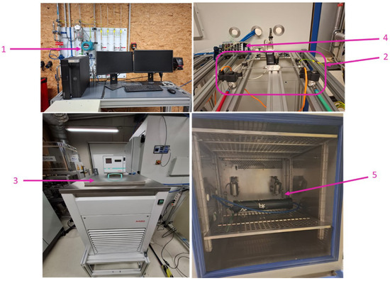
Figure 1.
Test bench.
The test bench is described as follows.
- Hydrogen Supply System
- A hydrogen flow controller regulates the flow of high-purity hydrogen (up to 99.99%) at pressures typically around 8 to 10 bar.
- The flow rate is adjustable to match specific absorption or desorption protocols.
- PID of Hydrogen Circuit System
- Pressure Sensors (Keller PA-33X series), Manufacturer: KELLER Druckmesstechnik AG, Winterthur, Switzerland: Installed to measure variations in pressure during hydrogen flow, offering an operational range of 0–100 bar.
- Thermocouples (type K): Attached to the tank’s surface to monitor temperature distribution at multiple points, with an operational range of −250 °C to +1250 °C.
- Mass Flow Controller (Brooks 5850S), Manufacturer: Brooks Instrument, Hatfield, PA, USA: Used to calculate the cumulative hydrogen mass absorbed or desorbed via integration of flow rates over time. The device is factory-calibrated and provides an accuracy of of full scale with a repeatability deviation of of the indicated rate.
- Heat Exchanger
- The Julabo F.P. 52 Refrigerated/Heating Circulator (Manufacturer: JULABO GmbH, Seelbach, Germany) precisely manages the tank’s temperature during tests. The circulator’s closed-loop control system relies on a Pt100 sensor (Manufacturer: JUMO GmbH & Co. KG, Fulda, Germany) to sample the temperature of the fluid as it exits the tank. This measurement is fed back into the circulator’s controller, which dynamically adjusts its heating and cooling output to maintain the circulating fluid at the prescribed setpoint.
- Data Acquisition and Control
- The entire system is managed by automated control software, National Instrument LabVIEW (version 18.0.1f2), enabling real-time monitoring and data logging of operational parameters.
- Users can define operating modes (absorption or desorption) and control parameters through a user interface.
- Climatic Chamber
- A chamber ensures consistent ambient conditions during testing, with the option to simulate varying environmental temperatures.
2.1. Data Collection
The test bench measures key variables such as hydrogen flow rate, pressure, and temperature during absorption and desorption processes. These variables constitute the input data set, while the SoC, derived from the mass of hydrogen stored, constitutes the output dataset. This data is essential for developing and validating offline estimation algorithms to ensure that they can reliably predict SoC under varying operating conditions.
Figure 2 illustrates the LabVIEW-based system interface used for data acquisition in the experimental test bench. This interface enables real-time monitoring and control of key operational parameters, including pressure, temperature, and hydrogen flow rate. The interface includes features such as mode selection (charge/discharge), cumulative hydrogen mass tracking, and temperature regulation through the heat exchanger.
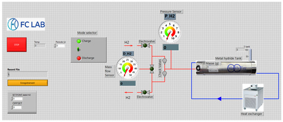
Figure 2.
LabVIEW Interface for Data Acquisition and System Control.
2.2. Operating Logic of the Test Bench
The working operation of the test bench consists in maintaining a constant hydrogen flow rate during both the charging (absorption) and the discharging (desorption) process. The process involves the following steps.
- □
- Charging Process
- •
- Hydrogen flow rate is defined and kept constant.
- •
- The charging cycle continues until the tank pressure reaches its maximum operational limit.
- •
- Heat generated during the exothermic absorption process is dissipated using a cooling circuit.
- □
- Discharging Process
- •
- Hydrogen is released until the tank pressure reaches ambient levels.
- •
- The endothermic desorption process requires heat input, supplied by the heat exchange circuit.
The recorded data from charging/discharging cycles represent the foundation datasets used for training and validation of the SoC estimation algorithms. It should be mentioned that the actual SoC values serve as the ground truth to evaluate the performance of the estimation models. During validation, the predicted SoC is compared with the known SoC from the dataset, allowing the computation of error metrics to quantify the accuracy of the models. The estimation algorithms are implemented and tested on the Matlab script R2023a, installed on a PC with: CPU Intel(R) i7-13800H @2.50 GHz, RAM 32 Go, and OS Win11 Education x64.
2.3. Database Description
The datasets used in this research were specifically generated to analyze the state of charge of metal hydride hydrogen storage tanks. Data was collected from experimental tests conducted for a hydrogen flow profile shown in Figure 3. The input features include external temperature (in °C), external pressure (in bar), and hydrogen flow rate (in Nl/min), while the output data represents SoC, calculated as
where denotes the initial hydrogen mass in the tank, the accumulated hydrogen mass at time t, and the maximum hydrogen mass. For all experiments, was set to zero. This assumption was validated by subjecting the tank to successive charge–discharge cycles until the volume of hydrogen withdrawn was sufficiently large that any remaining content could be regarded as negligible, thereby ensuring the tank was effectively empty prior to each test. is determined using the relationship between the molar flow rate, the volumetric flow rate and the mass flow rate of hydrogen as follows [18]:
where
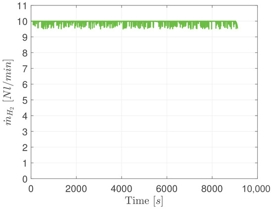
Figure 3.
Hydrogen flow rate vs. time.
- is the molar flow rate [];
- is the volumetric hydrogen flow rate [];
- is the molar volume of hydrogen at STP (0 °C, 1 atm) [];
- 60 is used to convert from min to s.
Then
The instantaneous mass rate expression is given by
Hence
where
- is the mass flow rate [];
- is the molar mass [];
- t is the time [].
SoC = 100% and SoC = 0% indicate that the hydrogen tank is full and empty, respectively. The datasets were sampled at 1-second intervals to reduce the number of data points, thereby decreasing computational complexity and processing time while maintaining sufficient resolution for model training and validation.
Data pre-processing is important to ensure robust performance and correct comparison of the estimator models, where feature normalization was performed using z-score scaling [19]. This method ensures that the input and output data have a mean of zero and a standard deviation of one, which helps improve the model’s convergence and performance. The standardization process is defined as
where and the are the input and output data, respectively. This approach ensures that all features and outputs are on the same scale. The same scaling factors derived from the training data were applied to the test data during evaluation. These collected data form the foundation for developing and validating offline SoC estimation techniques, which are detailed in the next section.
3. Offline Estimation Methods
3.1. Long Short-Term Memory
The LSTM neural network, an advanced architecture of the Recurrent Neural Network (RNN), is proposed to effectively overcome the vanishing gradient problem of the naively designed RNN by adding a memory cell structure [20]. A fundamental enhancement of the network architecture is achieved by replacing the standard recurrent hidden layer with an LSTM block. This substitution introduces a system of gates and internal memory cells that mitigate the vanishing-gradient problem, enabling the model to capture, retain, and leverage long-range temporal dependencies [8]. The architecture of LSTM is plotted as Figure 4 and can be represented by the following equations:
where f, i, c and o are the forget gate, input gate, remember cell and output gate, respectively, b denotes the bias, which is utilized to improve the flexibility of the model, and is the hidden layers data at time step t [21]. and represent the sigmoid and hyperbolic tangent activation functions; respectively, which are giving by
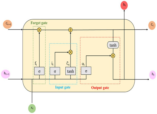
Figure 4.
Structure of an LSTM cell.
3.2. LSTM Algorithm for SoC Estimation
The state of charge of a hydrogen tank is heavily influenced by historical data, including temperature , pressure , and hydrogen flow rate . LSTM networks are well suited for capturing these temporal dependencies, as they excel at learning patterns and relationships in sequential data. Moreover, the input dataset for LSTM models must be structured as a three-dimensional (3D) array, defined by the format (Samples, Time Steps, and Features). Here, “Samples” refers to the number of sequences, “Time Steps” represents the number of observations within each sequence, and “Features” denotes the number of variables describing each observation. During the preprocessing step, the input dataset must be normalized and reshaped into this 3D format to serve as a suitable input for the network.
To fully leverage the sequential nature of the dataset, three different strategies were employed during the training of the LSTM model:
Full Dataset Injection: The entire dataset was fed into the model as a single sequence. This approach allows the LSTM to learn from global temporal trends across the dataset.
Dividing the dataset into Non-Overlapping Sequences: The dataset was segmented into fixed-length sequences, each representing a discrete window of time. By treating each sequence as an independent sample, the model could focus on specific localized patterns.
Using Overlapping Sequences: Overlapping windows were created by sliding the sequence window over the dataset with a defined step size. This method enhanced the model’s ability to learn smooth transitions and relationships between adjacent time segments.
The LSTM structure used for SoC estimation is illustrated in Figure 5. The model takes three input features, temperature, pressure, and hydrogen flow rate, which are passed through one or more LSTM layers (depending on the strategy employed to handle the input data). The output of the final LSTM layer is processed through a fully connected layer to generate the predicted SoC at each time step.
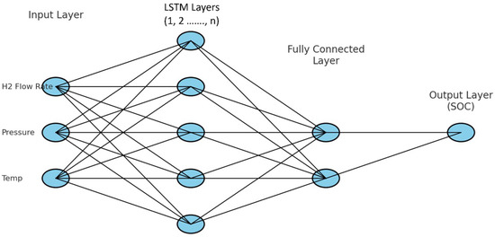
Figure 5.
LSTM model structure.
The hyperparameters of the three LSTM networks are set as shown in Table 1. As there is no clear method for determining the optimal values for key hyperparameters (such as the number of layers and units inside them, learning rate and training epochs), a trial-and-error approach is usually employed to identify the ideal model structure in these cases.

Table 1.
Hyperparameter tuning of LSTM networks.
Adam’s algorithm [22] has been applied as an optimization method for LSTM networks due to its high efficiency in computing and processing large amount of data and parameters. The loss function that is evaluated is
where n is the number of data points, is the actual value of SoC from the measurements, and is the estimated value from the LSTM network.
3.3. Support Vector Regression
Support Vector Regression (SVR) is a supervised learning algorithm derived from Support Vector Machines (SVMs) that is designed to predict continuous values. It works by finding a function that approximates the relationship between input and the output measurements while maintaining a margin of tolerance, , around the predictions. These functions, namely kernels, provide a modular framework that can be adapted to different tasks and domains by using different kernel function (i.e., linear, polynomial, sigmoid or radial basis) and the base algorithm [23]. SVR offers robust performance on small to medium-sized datasets by maximizing the margin and minimizing overfitting. However, it tends to perform poorly with large datasets due to its high computational complexity.
Support Vector Regression can be categorized into two primary types: -SVR and -SVR. For the first type, the optimization problem is solved by minimizing the following loss function [16,23]:
that is subject to
where
- w: Weight vector.
- b: Bias term.
- : Slack variables for handling deviations outside the margin.
- C: Regularization parameters controlling the trade-off between the margin (model flatness) and the magnitude of the slack variables.
- : Margin of tolerance around the predictions.
- L: Total number of data points used.
The constrained optimization problem of Equation (17) can be solved by applying Lagrange multipliers to Equations (18) and (19) using standard quadratic programming. The Support Vector Regression principle is illustrated in Figure 6, where the -insensitive tube and the support vectors are represented.
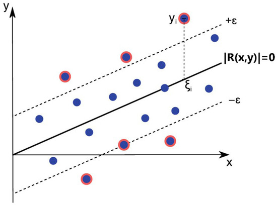
Figure 6.
SVR Visualization with Epsilon Tube and Support Vectors.
For the second type, -SVR; it is necessary to solve the following optimization problem, minimizing the following loss function [16,23]:
subject to the same constraints.
v is a parameter that controls the number of support vectors and training errors. The choice of SVR type depends on the dataset size and the desired balance between prediction accuracy and computational efficiency.
3.4. SVR for SoC Estimation
In this study, the same dataset used for LSTM estimation was utilized for SVR implementation, ensuring a consistent comparison of the two approaches. To provide a clear understanding of the SVR implementation, the flow of the code body is depicted in Figure 7.
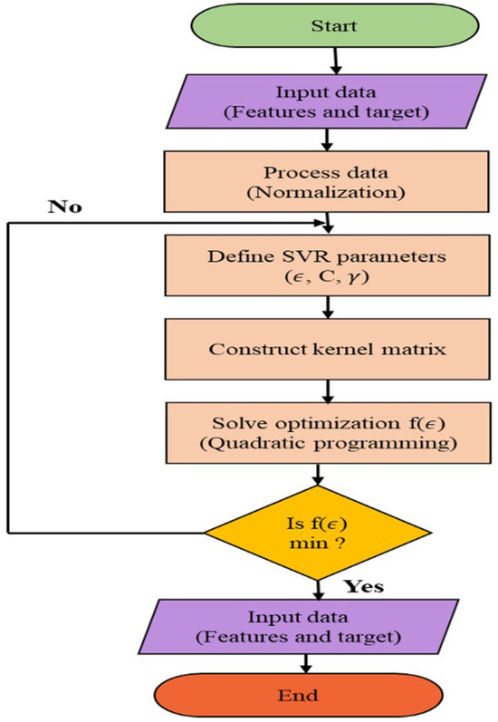
Figure 7.
The flowchart of SVR algorithm for SoC estimation.
To optimize the performance of the SVR model, a grid search approach [24] was employed to identify the best combination of hyperparameters. A predefined grid of values for C (regularization parameter), (epsilon tube for loss function), and (kernel scale for the RBF kernel) was tested. The grid search iterated over each combination of these parameters, training the SVR model with the corresponding settings. For each trained model, predictions were made on the training data, and the Root Mean Squared Error (RMSE) was calculated to evaluate the model’s performance.
where represents the actual SoC values, represents the predicted SoC values, and n is the total number of data points. The combination of parameters that resulted in the lowest RMSE was selected as the optimal configuration. The best-performing parameters were then stored and subsequently used in the final SVR implementation, ensuring the model operated with the most effective settings. Table 2 shows the optimal hyperparameters of the SVM model.

Table 2.
Optimal hyperparameters of SVR model.
4. Results and Discussion
The effectiveness of the implemented algorithms was evaluated using separate training and test datasets. The training dataset comprised 10,400 data points after removing outliers, while the independent test dataset contained 4800 new points spanning the same experimental ranges as the training data. Both datasets cover a temperature range of (18–22) °C, a pressure range of (0–8) bar, and a fixed hydrogen flow rate of 10 bar (Figure 3). The figures in the following sections present the results obtained from the test dataset.
4.1. State of Charge Estimation by LSTM Methods
As mentioned earlier, the input vector is defined as , where , , are the hydrogen flow rate, pressure and temperature of the hydrogen tank at time t, respectively. At first, LSTM is used with the full dataset injected at once as a single sequence for both charge and discharge cycles.
Figure 8 depicts the SoC estimation result for both charge (Figure 8a) and discharge cycles (Figure 8b) for the test datasets for the network described in Table 1. The results demonstrate acceptable performance, although the network initially struggles to accurately track the SoC trend, as the predicted SoC fails to match the initial starting point of the actual SoC. However, it quickly aligns with the actual SoC trend within a fraction of a second. During the charging phase, a slight noise is noticeable in the prediction between t = 800 s and t = 4000 s. After this interval, the prediction stabilizes and closely follows the actual SoC trend. In contrast, during the discharging phase, the noise is less pronounced, resulting in a more accurate prediction. This improvement is reflected in the lower RMSE value for the discharge phase compared to the charge phase.
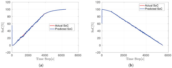
Figure 8.
LSTM SoC estimation results: (a) Charge (RMSE: 1.6858%). (b) Discharge (RMSE: 1.6358%).
To mitigate the cold start issue encountered in the full sequence method, a second LSTM network was implemented, where the dataset was partitioned into non-overlapping sequences. This approach allowed the network to process data in smaller, discrete chunks, enhancing its ability to capture localized patterns.
Figure 9 shows the results of SoC estimation for both charge (Figure 9a) and discharge (Figure 9b) cycles. Despite the sequence-based approach, the network continues to struggle with the initial SoC estimation. Nevertheless, the prediction quality improves markedly, closely tracking the actual SoC trend. Although minor noise is observed throughout the prediction, it does not significantly affect the overall prediction accuracy. With this network, the RMSE values of the charging and discharging phases are close to each other, indicating a similar prediction behavior for both phases.
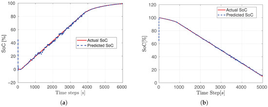
Figure 9.
LSTM SoC estimation results: (a) Charge (RMSE: 1.1739%). (b) Discharge (RMSE: 1.1544%).
The third LSTM implementation involved dividing the dataset into overlapping sequences, enabling the network to extract additional information from adjacent sequences. This strategy effectively addressed the cold start issue observed in earlier networks. The results of the SoC estimation are represented in Figure 10. The overlapping sequence method significantly mitigates the cold start problem, accurately predicting the initial SoC value. While some oscillations are observed along the prediction, the general behavior of the predicted SoC remains closely aligned with the actual SoC. This indicates that despite the oscillations, the network captures the underlying trend effectively, providing reliable estimations over the entire cycle. The RMSE values are close to those of the second network but remain lower compared to both networks, indicating an overall improvement in prediction accuracy.
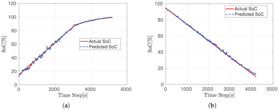
Figure 10.
LSTM SoC estimation results: (a) Charge (RMSE: 1.13395%). (b) Discharge (RMSE: 1.0786%).
4.2. Comparison of the Three LSTM Networks
The results of the three LSTM networks demonstrate varying levels of accuracy in estimating the State of Charge (SoC) during charge and discharge cycles. Network 1 achieves RMSE values of 1.6858% for the charge cycle and 1.6358% for the discharge cycle, making it the least accurate among the three. Network 2 shows improved performance with RMSE values of 1.1739% and 1.1544% for the charge and discharge cycles, respectively, reflecting better alignment between the predicted and actual SoC curves. Finally, Network 3 outperforms the others with the lowest RMSE values of 1.13395% for the charge cycle and 1.0786% for the discharge cycle, indicating the highest accuracy and closest match between predicted and actual SoC. Overall, Network 3 demonstrates superior performance in both charge and discharge scenarios, making it the most reliable estimator.
4.3. Experimental Results of SoC Estimation by SVR Algorithm
The SVR estimation employed the same test dataset used for the LSTM evaluation. Due to SVR’s computational constraints with large datasets, a reduced dataset was utilized for training, consisting of 9000 data points. Figure 11 presents the SoC estimation results for the discharge cycle. The SVR model demonstrates high accuracy, with no observable drift over time (Figure 11a). A zoomed-in view (Figure 11b) highlights the close alignment between the predicted and actual SoC throughout the estimation period.
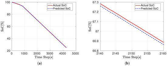
Figure 11.
SVR SoC estimation results: (a) Discharge (RMSE: 0.023329%). (b) A zoomed-in view.
Similar observations were made for the charging dataset, as illustrated in Figure 12. The primary difference lies at the onset of the estimation, where the predicted SoC remains null for a brief period, closely reflecting the actual SoC behavior. Once the SoC begins to increase, the SVR model closely tracks the actual trend (Figure 12a). A detailed view (Figure 12b) further underscores the minor discrepancies between the predicted and actual SoC values.
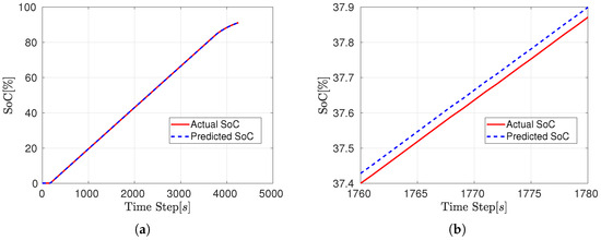
Figure 12.
SVR SoC estimation results: (a) Charge (RMSE: 0.028306%). (b) A zoomed-in view.
For both the charging and discharging phases, the recorded RMSE values are the lowest among the SoC estimators, indicating an excellent performance achieved by the SVR model.
4.4. Comparison Between LSTM and SVR
Both LSTM and SVR methods exhibited notable performance in SoC estimation, with distinct strengths and limitations. LSTM networks, particularly those employing overlapping sequences, demonstrated superior capability in handling large datasets and capturing long-term dependencies, making them suitable for scenarios involving extensive data volumes. However, LSTM networks showed susceptibility to noise and fluctuations in certain instances, which may affect prediction reliability. In contrast, SVR models excelled in providing stable and accurate predictions when applied to smaller datasets, offering high efficiency and minimal drift. Nevertheless, SVR’s performance diminished with larger datasets due to significant computational complexity, as depicted in Figure 13. Consequently, SVR is recommended for small to medium-sized datasets, while LSTM, especially with overlapping sequences, is preferable for large datasets requiring robust long-term dependency modeling.
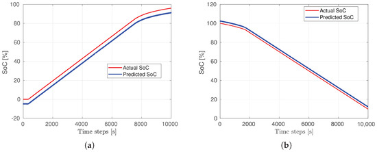
Figure 13.
SVR SoC estimation results for large datasets: (a) Charge (RMSE: 4.8178%). (b) Disharge (RMSE: 2.441%).
Figure 14 provides a consolidated comparison of SoC estimation performance across all methods, serving as a final synthesis of the preceding results. As shown, the SVR model consistently achieves the lowest RMSE, confirming its superior accuracy in both charge and discharge phases. Among the LSTM variants, Networks 2 and 3 deliver closely matched, substantially lower RMSE values than Network 1, which records the highest error. This summary plot thereby reinforces the earlier observations and highlights the relative merits of each approach.
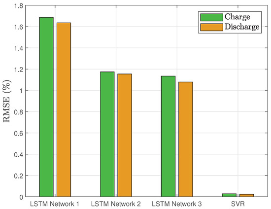
Figure 14.
The RMSE of SoC estimation for both charge and discharge cycles.
4.5. Assessment of Computing Burden
Computational cost is a critical constraint for state of charge estimation. In general, inference time depends on model complexity (e.g., number and size of layers), the volume of arithmetic operations (particularly matrix multiplications in recurrent units), the data segmentation strategy (continuous versus windowed sequences), and the processing hardware. This section compares the computation time of the four methods at each time step. Each measurement was repeated ten times, and the average per-step compute time is reported in Figure 15. The three LSTM variants exhibit the highest compute times, reflecting their internal gating and memory mechanisms. Network 1, which processes the entire dataset as a single continuous sequence, incurs the greatest burden (400 ms/step during charge), whereas Network 2—employing non-overlapping fixed-length windows—achieves the lowest LSTM latency (250 ms/step) by limiting its per-batch read size. Network 3, which uses overlapping windows, falls between these extremes (290 ms/step) due to the additional cost of re-processing overlapping segments. The SVR baseline is markedly more efficient (160 ms/step), owing to its sparse support vector representation and simpler prediction rule, although with reduced capacity to model temporal dependencies. Across all architectures, charge inference is consistently marginally slower than discharge, suggesting that absorption-phase inputs impose slightly greater computational overhead.
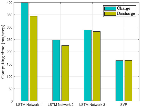
Figure 15.
The per-step computation time of the four deep learning networks.
5. Conclusions
This study demonstrates that classical battery estimation techniques can be successfully applied for the offline prediction of the state of charge (SoC) of metal hydride hydrogen storage tanks, addressing previously unmeasurable quantities. This approach pioneers the use of data-driven methods in hydrogen storage technology, addressing key challenges in state of charge estimation for metal hydride tanks. Three LSTM networks are developed to estimate the SoC by capturing temporal dependencies of key variables, including temperature, pressure, and hydrogen flow rate. These networks are trained on a dataset generated from multiple charge and discharge cycles of a functional hydrogen tank and are evaluated in terms of prediction accuracy and computational cost. The third network shows promising results in terms of accurately predicting the initial SoC, while the other two achieve better overall accuracy across cycles but struggle with initial SoC estimation. An SVR model was designed and tested on the same dataset, achieving low RMSE values of 0.0283% and 0.0233% for charge and discharge cycles, respectively, demonstrating high accuracy, smoothness, and efficiency in SoC prediction. However, its performance declined on larger datasets, revealing limitations for large-scale applications. Computational cost analysis showed that SVR is significantly more efficient than LSTM networks for both charge and discharge phases.
Future work will focus on developing and implementing online estimation methods for real-time applications, enabling continuous prediction of SoC as a function of hydrogen consumption in mobile systems such as hydrogen-powered vehicles. This is a significant challenge, as real-time estimation must account for instantaneous variations in hydrogen levels without relying on historical data, unlike the offline methods used in this study.
Author Contributions
Methodology, A.Y.; Software, A.Y.; Validation, D.C., S.L., A.N. and A.D.; Writing—original draft, A.Y.; Writing—review & editing, A.Y. and D.C.; Supervision, D.C., S.L., A.N. and A.D. All authors have read and agreed to the published version of the manuscript.
Funding
This work has been supported by the EIPHI Graduate School (contract ANR-17- EURE-0002) and the Region Bourgogne Franche-Comte within the framework of the ESYSH2 project.
Data Availability Statement
The original contributions presented in the study are included in the article, further inquiries can be directed to the corresponding authors.
Conflicts of Interest
The authors declare no conflicts of interest.
References
- Klopčič, N.; Grimmer, I.; Winkler, F.; Sartory, M.; Trattner, A. A review on metal hydride materials for hydrogen storage. J. Energy Storage 2023, 72, 108456. [Google Scholar] [CrossRef]
- Niaz, S.; Manzoor, T.; Pandith, A.H. Hydrogen storage: Materials, methods and perspectives. Renew. Sustain. Energy Rev. 2015, 50, 457–469. [Google Scholar] [CrossRef]
- Ravnsbœk, D.; Filinchuk, Y.; Cerenius, Y.; Jakobsen, H.J.; Besenbacher, F.; Skibsted, J.; Jensen, T.R. A series of mixed-metal borohydrides. Angew. Chem. Int. Ed. 2009, 48, 6659–6663. [Google Scholar] [CrossRef] [PubMed]
- Osman, A.I.; Mehta, N.; Elgarahy, A.M.; Hefny, M.; Al-Hinai, A.; Al-Muhtaseb, A.H.; Rooney, D.W. Hydrogen production, storage, utilisation and environmental impacts: A review. Environ. Chem. Lett. 2022, 20, 153–188. [Google Scholar] [CrossRef]
- Zhang, T.; Uratani, J.; Huang, Y.; Xu, L.; Griffiths, S.; Ding, Y. Hydrogen liquefaction and storage: Recent progress and perspectives. Renew. Sustain. Energy Rev. 2023, 176, 113204. [Google Scholar] [CrossRef]
- Hua, T.Q.; Roh, H.S.; Ahluwalia, R.K. Performance assessment of 700-bar compressed hydrogen storage for light duty fuel cell vehicles. Int. J. Hydrogen Energy 2017, 42, 25121–25129. [Google Scholar] [CrossRef]
- Marinescu-Pasoi, L.; Behrens, U.; Langer, G.; Gramatte, W.; Rastogi, A.K.; Schmitr, R.E. Hydrogen metal hydride storage with integrated catalytic recombiner for mobile application. Int. J. Hydrogen Energy 1991, 16, 407–412. [Google Scholar] [CrossRef]
- Javid, G.; Abdeslam, D.O.; Basset, M. Adaptive online state of charge estimation of evs lithium-ion batteries with deep recurrent neural networks. Energies 2021, 14, 758. [Google Scholar] [CrossRef]
- Zhu, D.; Chabane, D.; Ait-Amirat, Y.; N’Diaye, A.; Djerdir, A. Estimation of the state of charge of a hydride hydrogen tank for vehicle applications. In Proceedings of the 2017 IEEE Vehicle Power and Propulsion Conference (VPPC), Belfort, France, 11–14 December 2017; pp. 1–6. [Google Scholar] [CrossRef]
- Xing, Z.; Ma, G.; Wang, L.; Yang, L.; Guo, X.; Chen, S. Toward Visual Interaction: Hand Segmentation by Combining 3-D Graph Deep Learning and Laser Point Cloud for Intelligent Rehabilitation. IEEE Internet Things J. 2025, 12, 21328–21338. [Google Scholar] [CrossRef]
- Xing, Z.; Meng, Z.; Zheng, G.; Ma, G.; Yang, L.; Guo, X.; Tan, L.; Jiang, Y.; Wu, H. Intelligent rehabilitation in an aging population: Empowering human-machine interaction for hand function rehabilitation through 3D deep learning and point cloud. Front. Comput. Neurosci. 2025, 19, 1543643. [Google Scholar] [CrossRef] [PubMed]
- Chemali, E.; Kollmeyer, P.J.; Preindl, M.; Ahmed, R.; Emadi, A. Long Short-Term Memory Networks for Accurate State-of-Charge Estimation of Li-ion Batteries. IEEE Trans. Ind. Electron. 2018, 65, 6730–6739. [Google Scholar] [CrossRef]
- Chai, X.; Li, S.; Liang, F. A novel battery SOC estimation method based on random search optimized LSTM neural network. Energy 2024, 306, 132583. [Google Scholar] [CrossRef]
- Dubey, A.; Zaidi, A.; Kulshreshtha, A. State-of-Charge Estimation Algorithm for Li-ion Batteries using Long Short-Term Memory Network with Bayesian Optimization. In Proceedings of the 2022 Second International Conference on Interdisciplinary Cyber Physical Systems (ICPS), Chennai, India, 9–10 May 2022; pp. 68–73. [Google Scholar] [CrossRef]
- Hu, J.N.; Hu, J.J.; Lin, H.B.; Li, X.P.; Jiang, C.L.; Qiu, X.H.; Li, W.S. State-of-charge estimation for battery management system using optimized support vector machine for regression. J. Power Sources 2014, 269, 682–693. [Google Scholar] [CrossRef]
- Shi, Q.S.; Zhang, C.H.; Cui, N.X. Estimation of battery state-of-charge using ν-support vector regression algorithm. Int. J. Automot. Technol. 2008, 9, 759–764. [Google Scholar] [CrossRef]
- Jumah, S.; Elezab, A.; Zayed, O.; Ahmed, R.; Narimani, M.; Emadi, A. State of Charge Estimation for EV Batteries Using Support Vector Regression. In Proceedings of the 2022 IEEE/AIAA Transportation Electrification Conference and Electric Aircraft Technologies Symposium (ITEC+EATS), Anaheim, CA, USA, 15–17 June 2022; pp. 964–969. [Google Scholar] [CrossRef]
- Chabane, D.; Harel, F.; Djerdir, A.; Candusso, D.; ElKedim, O.; Fenineche, N. A new method for the characterization of hydrides hydrogen tanks dedicated to automotive applications. Int. J. Hydrogen Energy 2016, 41, 11682–11691. [Google Scholar] [CrossRef]
- Cabello-Solorzano, K.; Ortigosa de Araujo, I.; Peña, M.; Correia, L.; Tallón-Ballesteros, A.J. The Impact of Data Normalization on the Accuracy of Machine Learning Algorithms: A Comparative Analysis. In Proceedings of the 18th International Conference on Soft Computing Models in Industrial and Environmental Applications (SOCO 2023), Salamanca, Spain, 5–7 September 2023; pp. 344–353. [Google Scholar]
- Bian, C.; He, H.; Yang, S. Stacked bidirectional long short-term memory networks for state-of-charge estimation of lithium-ion batteries. Energy 2020, 191, 116538. [Google Scholar] [CrossRef]
- Ma, L.; Hu, C.; Cheng, F. State of Charge and State of Energy Estimation for Lithium-Ion Batteries Based on a Long Short-Term Memory Neural Network. J. Energy Storage 2021, 37, 102440. [Google Scholar] [CrossRef]
- Kingma, D.P.; Ba, J. Adam: A Method for Stochastic Optimization. In Proceedings of the 2014 International Conference on Learning Representations, Banff, AB, Canada, 14–16 April 2014. [Google Scholar]
- Álvarez Antón, J.C.; Nieto, P.J.G.; de Cos Juez, F.J.; Lasheras, F.S.; Vega, M.G.; Gutiérrez, M.N.R. Battery state-of-charge estimator using the SVM technique. Appl. Math. Model. 2013, 37, 6244–6253. [Google Scholar] [CrossRef]
- Alibrahim, H.; Ludwig, S.A. Hyperparameter Optimization: Comparing Genetic Algorithm against Grid Search and Bayesian Optimization. In Proceedings of the 2021 IEEE Congress on Evolutionary Computation (CEC), Kraków, Poland, 28 June–1 July 2021; pp. 1551–1559. [Google Scholar] [CrossRef]
Disclaimer/Publisher’s Note: The statements, opinions and data contained in all publications are solely those of the individual author(s) and contributor(s) and not of MDPI and/or the editor(s). MDPI and/or the editor(s) disclaim responsibility for any injury to people or property resulting from any ideas, methods, instructions or products referred to in the content. |
© 2025 by the authors. Licensee MDPI, Basel, Switzerland. This article is an open access article distributed under the terms and conditions of the Creative Commons Attribution (CC BY) license (https://creativecommons.org/licenses/by/4.0/).