Abstract
This paper introduces an intelligent fault-diagnosis framework for power transformers that integrates hybrid machine-learning models with nature-inspired optimization. Current signals were acquired from a laboratory-scale three-phase transformer under both healthy and various fault conditions. A suite of 41 discriminative features was engineered from time–frequency and sparse representations generated via Discrete Wavelet Transform (DWT) and Matching Pursuit (MP). The resulting dataset of 2400 labeled segments was used to develop four hybrid models, PSO-SVM, PSO-RF, BA-SVM, and BA-RF, wherein Particle Swarm Optimization (PSO) and the Bees Algorithm (BA) served as wrapper optimizers for simultaneous feature selection and hyperparameter tuning. Rigorous evaluation with 5-fold and 10-fold cross-validation demonstrated the superior performance of Random Forest-based models, with the BA-RF hybrid achieving peak performance (98.33% accuracy, 99.09% precision). The results validate the proposed methodology, establishing that the fusion of wavelet- and MP-based feature extraction with metaheuristic optimization constitutes a robust and accurate paradigm for transformer fault diagnosis.
1. Introduction
Power transformers represent indispensable assets within electrical power systems, fulfilling the critical functions of voltage regulation, load management, and ensuring the reliable continuity of electricity supply [1]. Given their pivotal role, any fault condition or operational malfunction can precipitate severe consequences, including widespread system instability, protracted power outages, and substantial equipment damage [2]. Consequently, the advancement of accurate, efficient, and intelligent diagnostic methodologies for transformer condition monitoring has emerged as a paramount objective within both academic research and industrial practice [3,4].
Conventional transformer protection schemes predominantly rely on threshold-based mechanisms and frequency-domain analysis techniques [5]. While established, these methods exhibit inherent limitations, particularly in their capacity to reliably discriminate between benign transient phenomena, such as magnetizing inrush currents, and genuine internal fault conditions [6,7]. This diagnostic ambiguity is exacerbated under dynamic system operations, potentially leading to either nuisance tripping or a failure to operate—both of which compromise system reliability. This shortfall has catalyzed significant interest in leveraging data-driven artificial intelligence (AI) and machine learning (ML) paradigms, which offer superior capabilities in identifying complex, non-linear patterns within operational data [8,9].
Among ML classifiers, Support Vector Machines (SVMs) and Random Forests (RFs) have demonstrated considerable promise in power system fault diagnosis and pattern recognition tasks [10,11]. Nevertheless, the efficacy of these models is contingent upon two critical factors: the selection of optimal hyperparameters and the extraction of salient features from raw signal data. To address the former, nature-inspired optimization algorithms such as Particle Swarm Optimization (PSO) and the Bees Algorithm (BA) have been increasingly adopted to automate and enhance the hyperparameter tuning process, thereby improving model generalization and performance [12,13].
Simultaneously, the challenge of feature extraction is adeptly met by advanced signal processing techniques. The Discrete Wavelet Transform (DWT) is particularly well-suited for analyzing non-stationary power system signals, as it facilitates multi-resolution analysis in both the time and frequency domains. By decomposing current and voltage waveforms, DWT enables the derivation of a compact and highly discriminative feature set that accurately characterizes transient fault signatures [14,15]. Table 1 summarises the approaches for transformer fault diagnosis proposed in the literature.

Table 1.
Representative approaches for transformer fault diagnosis.
Building upon these foundations, this paper proposes a comprehensive hybrid intelligent framework for power transformer fault classification. The proposed methodology integrates DWT-based feature extraction with metaheuristic-optimized machine learning. Specifically, the authors formulate and evaluate four distinct hybrid models: PSO-SVM, PSO-RF, BA-SVM, and BA-RF. These models are rigorously trained and validated using empirical data acquired from a laboratory-scale three-phase power transformer, subjected to a range of both healthy and faulty operating conditions. Model performance is critically assessed through robust k-fold cross-validation (5-fold and 10-fold) and evaluated against a comprehensive suite of performance metrics, including Accuracy, Precision, Recall, F1-Score, Specificity, and Negative Predictive Value (NPV), to ensure a statistically sound and holistic evaluation of diagnostic capability.
The principal contributions of this work are delineated as follows:
- Empirical dataset utilization. The authors validate the approach on a real experimental dataset of current signals from a laboratory three-phase power transformer under comprehensive healthy and faulty operating conditions.
- Advanced feature extraction. A discriminative 41-feature set is engineered using Discrete Wavelet Transform (DWT) and Matching Pursuit (MP) to capture complementary time–frequency and sparse-dictionary characteristics.
- Novel hybrid models. We develop four hybrid intelligent models by integrating SVM and RF classifiers with the nature-inspired optimizers PSO and the Bees Algorithm (BA).
- Rigorous performance validation. The authors employ 5-fold and 10-fold cross-validation to assess robustness, mitigate overfitting, and demonstrate generalization across accuracy, precision, recall, and F1-score.
- Behavioral analysis. Convergence and feature-importance analyses explain PSO’s faster early ascent and BA’s steadier late-stage refinement, clarifying why BA-RF attains the best overall performance.
The remainder of this manuscript is structured as follows: Section 2 delineates the experimental framework, detailing the laboratory setup, the data acquisition methodology, and the procedures for feature extraction. Section 3 elaborates on the proposed methodological approach, encompassing the signal processing techniques, the architecture of the developed hybrid models, and the implementation of the optimization algorithms. Section 4 presents a comprehensive analysis of the experimental results, including a comparative performance evaluation of the proposed models. Finally, Section 5 provides concluding remarks, summarizes the key findings, and suggests promising avenues for future research.
Literature Review
Taxonomy of approaches. Related work on transformer fault diagnosis spans five families:
- (i)
- Classical analyses—FRA, DGA, STFT: mature and interpretable but limited for short transients and mixed events.
- (ii)
- Engineered-feature ML—SVM, k-NN, RF on time–frequency features (e.g., DWT): strong when features capture transient energy but sensitive to hyperparameters.
- (iii)
- Gradient-boosted trees—XGBoost/LightGBM: state-of-the-art tabular learners with efficient inference; require careful regularization on small datasets.
- (iv)
- Stacking/ensembles—meta-learners (e.g., logistic or meta-RF) over RF/SVM/XGB: can add incremental gains but increase complexity/latency.
- (v)
- Deep learning—1D-CNNs, LSTMs, Transformers on raw waveforms: learn features end-to-end, typically needing larger, diverse datasets and careful deployment on embedded hardware.
Comparative insights. Multi-resolution features (e.g., DWT bands) consistently improve separability of internal vs. external faults. Among classical ML models, RF and XGB often top SVM/k-NN on tabular features; stacking can help but at the cost of added inference and maintenance complexity. Deep models excel with large, varied data and augmentation but can struggle to generalize across hardware/noise domains without domain adaptation.
Gap and motivation. Many studies optimize only hyperparameters or only feature subsets; few unify DWT with sparse (MP) features and wrapper-based joint optimization while validating on real experimental signals with both 5-fold and 10-fold cross-validation. Our work addresses this gap by coupling PSO and the Bees Algorithm (BA) with RF and SVM to jointly select features and tune hyperparameters, then demonstrating that RF-based hybrids generalize the best across folds (with BA-RF top under 10-fold CV; PSO-RF close behind).
Positioning of the present study. The authors target a deployment-minded pipeline—low-latency inference, interpretable feature importance, and robustness under limited, laboratory-scale data—where engineered DWT + MP features and tree ensembles are a pragmatic fit. We analyze convergence (PSO faster early, BA steadier late) and feature importance to explain model behavior, aligning the methodology with practical substation use cases.
2. Research Methodology
2.1. Experimental Setup
To empirically validate the proposed fault diagnosis methodology, a dedicated experimental testbed centered on a three-phase power transformer was constructed under controlled laboratory conditions. The setup was designed to accurately replicate both healthy and a comprehensive range of fault scenarios. The core components of the testbed are detailed below:
- Transformer Specifications: The core component was a 5 kVA, 416/240 V three-phase transformer, selected to model realistic operational and fault conditions encountered in practical settings.
- Fault Simulation Unit: A programmable switching system, integrating electromechanical relays and protective resistances, was engineered to induce controlled fault events. The unit was capable of generating various internal and external fault types, including Line-to-Ground (LG), Line-to-Line (LL), Turn-to-Turn (TT), and Single Line-to-Ground (SLG) faults.
- Data Acquisition System (DAQ): A National Instruments cDAQ-9178 with an NI-9205 analog input module acquired current and voltage at 250 kS/s (per channel). This high-rate capture preserves microsecond-scale transients and provides headroom for offline anti-alias filtering and controlled resampling used in the ML pipeline.
- Sensor Configuration: Measurement precision was ensured through the use of high-accuracy transducers: LEM LA 55-P current sensors (with ±0.5% accuracy) and LEM LV 25-P voltage sensors (with ±0.2% accuracy).
- Software Integration: A centralized LabVIEW 2024 Q1 platform provided real-time monitoring, automated data logging, and post-processing capabilities. Custom scripts were developed to manage fault initiation, ensuring precise synchronization between fault events and signal acquisition. The equipment required to conduct this research has been provided by Cardiff University at the Electric Machine Laboratory (Cardiff, UK).
The integrated experimental configuration, illustrated in Figure 1, synergizes the DAQ system, current transformers (CTs), relay modules, and control interface. This comprehensive arrangement guarantees the repeatability of experiments, data reliability, and operational safety throughout the fault simulation and data collection process.
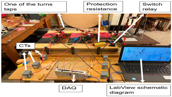
Figure 1.
Schematic of the experimental apparatus for transformer fault diagnosis.
Figure 2 depicts the laboratory-scale experimental configuration, which features a three-phase power transformer specifically designed for fault simulation and data acquisition. The low-voltage windings are furnished with tap connections, providing configurational flexibility that enables controlled fault induction through the reconfiguration of inter-winding electrical pathways. These access points facilitate the systematic emulation of diverse internal and external fault scenarios by permitting precise adjustments to the electrical topology between winding segments.
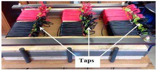
Figure 2.
Schematic of the multi-tap winding for inter-turn fault emulation.
The transformer assembly is securely mounted on a rigid wooden frame. Laminated iron cores are positioned beneath the windings to ensure consistent magnetic flux linkage and operational stability. This carefully engineered setup supports controlled, repeatable experimentation, thereby enabling the acquisition of high-fidelity datasets essential for the development and validation of advanced fault classification algorithms in power system diagnostics.
2.2. Fault Simulation and Data Collection
To evaluate the efficacy of the proposed methodology, a series of common transformer fault conditions were systematically simulated, as summarized in Table 2. Fault events were induced via programmable switch relays, and real-time signal variations were captured using a LabVIEW-controlled data acquisition system. Signals were acquired at 250 kS/s (Section 2.1) and then down sampled to 1 kHz for machine-learning (ML) analysis. To prevent aliasing, we used a two-stage decimation: 25× (250 kS/s → 10 kS/s) followed by 10× (10 kS/s → 1 kHz). Each stage applied zero-phase (forward–backward) low-pass filtering before decimation. In the final stage, a 5th-order Butterworth low-pass with 500 Hz cutoff (−3 dB) was used. This procedure ensures that only band-limited content enters the 1 kHz stream while preserving the dynamics relevant to power-frequency phenomena and their lower harmonics.
Table 2.
Performance Evaluation of the Proposed Method for Different Fault Types.
Effective bandwidth entering the ML pipeline, 0–500 Hz (−3 dB at 500 Hz) with a practically flat passband to ~450 Hz. Frequencies above 500 Hz are strongly attenuated prior to resampling and are therefore excluded from feature extraction and classification.
Rationale for bandwidth and rate, fault-related energy for our laboratory transformer is concentrated around the 50 Hz fundamental and its lower harmonics (<10th, ≤500 Hz). Capturing at 250 kS/s guarantees transient fidelity and precise event timing, whereas 1 kHz (after anti-aliasing) provides a noise-reduced, compact representation that is well matched to our feature set and classifiers.
2.3. Dataset Description
The experimental data were collected from a three-phase, 5 kVA, 416/240 V power transformer located in the high-voltage laboratory. A controlled fault simulation setup was developed to generate six fault categories, including one healthy condition and five types of winding and core faults. The current signals were captured using current transformers (CTs) and a data acquisition (DAQ) unit (e.g., NI USB-6218).
Each signal was sampled at 1 kHz and segmented into shorter windows for analysis. A total of 2400 samples were used, distributed as shown in Table 3.
Table 3.
Summary of dataset description.
The dataset was divided into 70% for training, 15% for validation, and 15% for testing. All signals were normalized between 0 and 1 before feature extraction to ensure numerical stability.
2.4. Synthetic-Signal Validation (Protocol and Summary)
To complement laboratory validation, we synthesized currents as:
With class-specific perturbations:
- internal faults: phase-selective amplitude surge + DC offset + high-frequency transient burst.
- external faults: shorter transient with lower harmonic spread.
- healthy: stationary with modest harmonic content.
- nuisance events (inrush-like): strong low-frequency offset and saturation-like distortion.
Signals were sampled at 10 kHz, segmented as in the lab data, and processed by the same DWT/MP + PSO/BA-optimized classifiers. The RF-based hybrids retained the highest accuracy; BA-RF delivered the most stable results across seeds, while PSO converged faster.
2.5. Data Processing and Feature Extraction
The acquired current and voltage signals were processed using Discrete Wavelet Transform (DWT) to extract discriminative time–frequency features that characterize both transient and steady-state behaviors. Following feature extraction, Particle Swarm Optimization (PSO) and the Bees Algorithm (BA) were employed to optimize feature selection, thereby reducing dimensionality and enhancing the generalization capability and performance of the subsequent classifiers.
2.6. Signal Decomposition and Feature Extraction
The DWT was applied using the Daubechies 4 (db4) mother wavelet due to its good localization properties for transient signals. Each signal was decomposed into five levels, and the detail coefficients were used for feature computation.
The Matching Pursuit (MP) algorithm further decomposed each signal into adaptive atoms based on a Gabor dictionary, enabling precise time–frequency analysis. From each sub-band, 17 features were extracted, including statistical measures (mean, variance, skewness, kurtosis), energy entropy, and wavelet packet energy ratios.3.1 Wavelet-Based Feature Extraction.
The Wavelet Transform (WT) was employed to derive a time–frequency representation of the acquired current signals. A multi-level decomposition was executed utilizing a 4 (db4) mother wavelet across four levels. This process effectively isolates the signal’s constituent high-frequency and low-frequency components, thereby capturing transient phenomena that are critical for discriminating between fault conditions and healthy operational states [27,28].
Consistency of DWT band interpretation, Wavelet features were computed after resampling to 1 kHz, so the dyadic detail bands are:
d1: 250–500 Hz, d2: 125–250 Hz, d3: 62.5–125 Hz, d4: 31.25–62.5 Hz, and a4: 0–31.25 Hz (sym4, 4 levels). All results and figures in this paper refer to these bands, which align with the 0–500 Hz effective bandwidth of the ML pipeline.
As illustrated in Figure 3, the decomposition yields a set of approximation (a4) and detail (d1–d4) coefficients. This multi-resolution analysis provides a hierarchical representation of the signal, facilitating the extraction of both overarching trends (global features) and localized, transient events (local features) for subsequent diagnostic analysis.
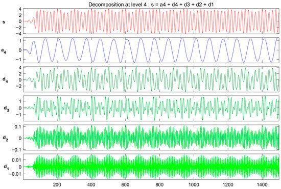
Figure 3.
DWT decomposition of signal (s) yielding transient-free approximation (a4) and detail (d1–d4) coefficients.
2.7. Matching Pursuit (MP) Dictionary-Based Sparse Signal Representation
The reconstruction of the original current waveform via Matching Pursuit (MP) was employed to assess the fidelity of the sparse approximation. MP operates through an iterative greedy selection: in each step, the atom from a predefined dictionary exhibiting the highest correlation with the current residual is selected, and the residual is updated. This procedure yields a compact linear combination of atoms, terminating when a specified error threshold or sparsity constraint is met, thereby balancing maximal energy retention against minimal ℓ2-norm reconstruction error [29,30].
At convergence (iteration 500), the approximation achieved a retained energy of 100%, verifying that the essential informational content of the source signal was wholly conserved. The process resulted in exceptionally low relative errors across all evaluated norms, quantitatively confirming the high precision of the reconstruction:
- L2 Norm Error: 0.07%
- L∞ (Maximum) Norm Error: 0.17%
- L1 Norm Error: 0.07%
To elucidate the structural composition of the sparse signal approximation, the constituent atoms selected from the dictionary are delineated in Figure 4. This set comprises elements drawn from multiple analytic domains: wavelet functions (specifically sym4 and wpsym4), the Discrete Cosine Transform (DCT), and canonical sinusoidal basis functions (sine and cosine).
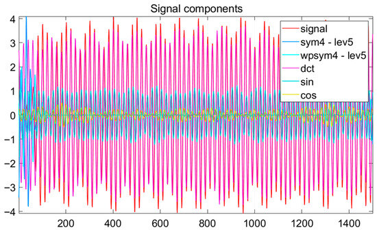
Figure 4.
Decomposed signal components reconstructed via sparse coding over multiple dictionaries. The combined sum of these components yields the complete signal approximation.
The original signal is depicted in red, with the contribution of each atomic type distinctly visualized. A high-intensity concentration of wavelet-based atoms is observed, underscoring their predominant efficacy in representing transient phenomena and oscillatory patterns inherent to the current signal. Concurrently, sinusoidal and DCT components provide complementary representations of lower-frequency harmonic content, thereby enhancing the overall fidelity of the reconstruction. Figure 5 explains the Signal and its approximation from a reconstruction process.
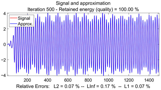
Figure 5.
Signal and its approximation from a reconstruction process (Iteration 500). The retained energy is 100%, with minimal relative errors (L2 = 0.07%, L∞ = 0.17%, L1 = 0.07%), indicating an exceptionally accurate reconstruction.
This synergistic integration of heterogeneous basis functions facilitates a parsimonious yet highly expressive signal representation, capable of encapsulating both localized transient features and overarching global trends with high precision.
The distribution of indices corresponding to the selected atoms is presented in Figure 6. The visualization reveals a pronounced predominance of wavelet-based atoms within the sparse representation. From a dictionary encompassing 6005 potential atoms, the approximation was achieved using a markedly compact set of only 500 elements. This substantial reduction—retaining merely 5.4% of the available atoms—exemplifies the parsimony and efficiency of the sparse coding process, confirming its ability to distill the most salient features of the signal into a minimal number of highly informative components.

Figure 6.
Indices of the most informative coefficients selected from multiple transform domains (e.g., Wavelet, Fourier, DCT) for the task of feature extraction and dimensionality reduction. The convergence behavior of the sparse approximation process is illustrated in Figure 7.
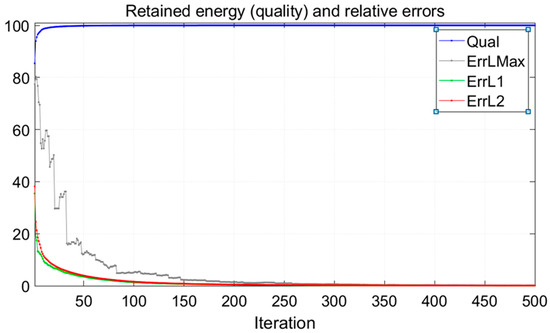
Figure 7.
Retained energy (blue) reaches 100% as L1, L2, and L∞ errors decrease to zero, confirming stable convergence to an accurate solution.
The plot demonstrates the asymptotic progression of retained signal energy toward 100%, concurrent with the rapid decay of the relative error norms—specifically the L1, L2, and maximum (L∞) norms. This simultaneous convergence of high energy retention and diminishing reconstruction error signifies a highly efficient and accurate signal representation, achieving optimal fidelity with minimal computational overhead.
Finally, the residual signal, plotted in Figure 8, exhibits consistently low amplitude across the entire time series. This minimal discrepancy between the original and reconstructed waveforms conclusively verifies that the sparse approximation successfully preserved the essential characteristics of the original signal with negligible information loss. The absence of significant structural features in the residual further affirms the comprehensiveness of the extracted atomic representation.
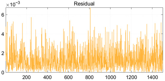
Figure 8.
The residual signal, defined as the difference between the original and reconstructed signals, representing the approximation error of the model.
2.8. Classification Techniques
To facilitate the classification of extracted features and enable the accurate identification of power transformer faults, two well-established supervised machine learning algorithms were implemented: Support Vector Machine (SVM) and Random Forest (RF).
2.8.1. Support Vector Machine (SVM)
Support Vector Machine (SVM) is a supervised learning algorithm designed to determine the optimal hyperplane that maximizes the margin between data points of distinct classes [31]. This method is especially effective for high-dimensional data and can address non-linear separability through the use of kernel functions, such as the radial basis function (RBF), which project data into higher-dimensional spaces where linear separation becomes feasible. The algorithm identifies a critical subset of training examples, known as support vectors, that define the decision boundary. Renowned for its strong generalization performance and resistance to overfitting, SVM is particularly well-suited for fault classification in complex systems like power transformers, where distinguishing between subtle fault signatures and normal operating conditions is essential [32].
The SVM classifier aims to find the optimal decision boundary (hyperplane) that maximizes the margin between two classes. For a binary classification problem, the decision function is:
where x denotes the input feature vector, represents the support vectors selected from the training data, and are the corresponding class labels. The coefficients are the Lagrange multipliers that weight each support vector’s contribution. The function is a kernel function that maps the input data into a higher-dimensional space—commonly, a radial basis function (RBF) kernel is used for non-linear separation. Finally, b is the bias term that adjusts the position of the decision boundary.
For the Radial Basis Function (RBF) kernel:
where controls the width of the Gaussian kernel.
2.8.2. Random Forest (RF)
Random Forest (RF) is an ensemble classifier that builds multiple decision trees and aggregates their predictions to make final decisions. Each individual tree is trained on a different bootstrapped subset of the data and operates independently. The final predicted class is obtained through majority voting across all trees. To ensure model diversity and prevent overfitting, RF randomly selects a subset of features at each node when determining the optimal split. The selected feature is the one that maximizes the information gain, thus enhancing the discriminative power of the tree. This combination of bagging and random feature selection contributes to RF’s high accuracy, robustness, and ability to handle complex and high-dimensional datasets [33,34].
Individual Tree Prediction:
Each decision tree in the forest is trained on a bootstrapped sample of the data and produces a prediction for input Ensemble Prediction (Majority Voting):
The final output is determined by aggregating the predictions of all trees using majority voting.
Feature Selection at Node Splitting:
At each node, a subset of randomly selected features is evaluated, and the feature that maximizes the information gain (e.g., Gini index or entropy reduction) is chosen for the split.
2.9. Feature Selection
To improve classification performance and reduce computational complexity, feature selection was performed using two nature-inspired metaheuristic algorithms: Particle Swarm Optimization (PSO) and the Bees Algorithm (BA). These algorithms were used to search for the optimal subset of features from the extracted wavelet and sparse representation features.
2.9.1. Particle Swarm Optimization (PSO)
The (PSO) algorithm, introduced by Eberhart and Kennedy [35], is a widely recognized metaheuristic optimization technique inspired by the collective social behaviors observed in nature, such as bird flocking and fish schooling. Within this paradigm, each particle embodies a potential solution and iteratively adjusts its position according to both its individual historical best performance and the best solution identified within its neighborhood. This dual-influence mechanism emulates the adaptive and collaborative dynamics characteristic of biological groups. As a result of this robust and efficient search strategy, PSO has established itself as a highly versatile method capable of addressing a diverse spectrum of complex optimization challenges [36]. The structured procedure for determining the optimal solution is delineated as follows:
- (a)
- Initialization: The algorithm commences by initializing a population of particles, each assigned a randomized position and velocity within the feasible search domain. The fitness of each particle is evaluated based on the objective function. The particle exhibiting the highest fitness is designated the global best (), while each particle individually records its own best-performing position as its personal best ().
- (b)
- Velocity Update: During iterative cycles, each particle’s velocity is updated according to a weighted combination of its current velocity, cognitive attraction to its , and social attraction to the swarm’s . This update mechanism facilitates a balanced exploration of the search space while progressively exploiting regions of high fitness, effectively guiding the collective toward optimal solutions.
- (c)
- Position Update: Using the newly computed velocity, each particle’s position is updated. This movement is mathematically formalized (see Equation (7)), ensuring structured progression through the solution space. The iterative process of velocity and position updates continues until convergence criteria are satisfied, thereby refining the swarm’s proximity to the global optimum.
- (d)
- Update of Best Values: Following the evaluation of new positions, each particle’s fitness is compared against its historical performance. If a particle’s current position yields a superior fitness value, its personal best () is updated to this new position. Concurrently, the global best () is revised should any particle discover a solution exceeding the fitness of the current . This selection mechanism is formally governed by the criteria specified in Equation (8).
- (e)
- Termination Check: The algorithm assesses whether predefined termination conditions—such as reaching a maximum number of iterations or achieving a satisfactory fitness threshold—have been met. If satisfied, the optimization process halts, and the current is returned as the final solution. Otherwise, the procedure reverts to the velocity update phase (Step b), perpetuating the iterative cycle until convergence is attained.
The PSO parameters used in this study are summarized in Table 4, and PSO Symbols are shown in Appendix A: Table A1.
Table 4.
PSO parameters.
The Particle Swarm Optimization (PSO) procedure, summarized in Figure 9, initializes a swarm with random positions and velocities. Each particle’s fitness is evaluated, and both personal () and global best () positions are updated iteratively. Velocities are adjusted based on cognitive and social components until a stopping criterion is satisfied, at which point gbest is returned as the optimal solution.
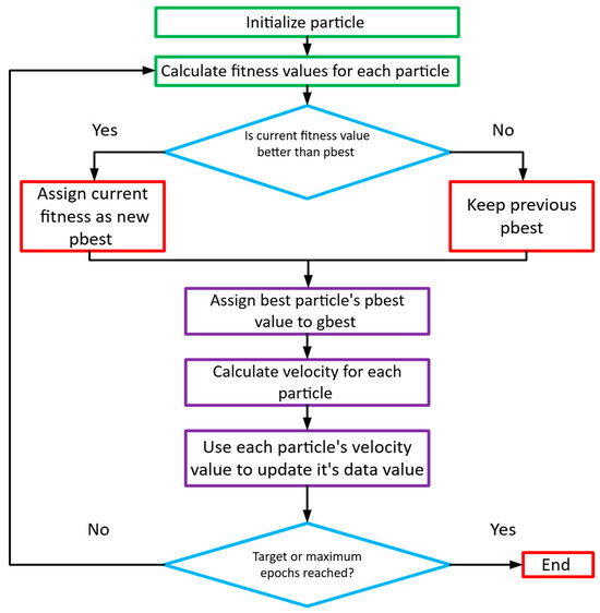
Figure 9.
The PSO Algorithm flowchart.
2.9.2. Bees Algorithm (BA)
The Bees Algorithm (BA) is a metaheuristic optimization technique grounded in the foraging behavior of honeybee colonies [37]. As a population-based search method, it emulates the natural processes of scouting, recruitment, and exploitation observed in bee swarms to address complex optimization problems [38]. The algorithm systematically balances global exploration with localized refinement through the strategic management of six core control parameters:
- Number of Scout Bees (ns): Defines the initial population size dispersed throughout the search space to promote broad exploration.
- Number of Selected Sites (m): Indicates the quantity of the most promising regions identified by scouts and chosen for intensified investigation.
- Number of Elite Sites (e): Specifies the top-performing sites among the selected ones, which receive the greatest allocation of computational resources.
- Number of Bees Recruited for Elite Sites (nep): Determines the population size assigned to conduct focused local searches around each elite site to enhance exploitation.
- Number of Bees Recruited for Non-Elite Selected Sites (nsp): Allocates bees to promising but non-elite sites, maintaining a balance between exploration and exploitation.
- Neighborhood Size (ngh): Governs the spatial extent of local searches around selected sites, typically contracting over time to improve solution precision.
The search process commences with the random distribution of a predefined number of scout bees (ns) across the solution space. Each site visited by a scout is evaluated using the objective function and ranked in either ascending or descending order, corresponding to minimization or maximization problems, respectively. From this ranked list, the most promising sites are designated as selected sites (m). These are further categorized into elite sites (e), which exhibit the highest fitness, and non-elite sites (m − e).
Subsequently, neighborhood searches are initiated around these selected sites. A larger contingent of forager bees (nep) is deployed to intensively exploit the regions surrounding each elite site, while a smaller number of bees (nsp) is assigned to explore the neighborhoods of non-elite sites. This differential allocation ensures a balanced emphasis on both refinement of high-quality solutions and broader exploration of the search space. The assignment of bees is governed by the following expressions:
Equation (11) specifies the primary constraint governing the Bees Algorithm, requiring that the number of elite sites e does not exceed the number of selected sites m. The total population size p is subsequently determined using Equation (12), which aggregates the bees allocated to elite sites, non-elite sites, and random scout bees. The expression for the number of randomly distributed scout bees during initialization, which also encompasses unselected bees, is given by:
Within the framework of this algorithm, the variable “rand” corresponds to a stochastically generated vector component uniformly distributed within the interval [0, 1], while and respectively delineate the lower and upper boundaries of the feasible solution domain. During the neighborhood search phase, the recruitment of bees is governed by the following positional update mechanism:
The Bees Algorithm (BA) can be formally defined as an iterative search process aimed at determining the optimal solution to an optimization problem. Mathematically, this objective is expressed as follows:
where denotes the objective function(s); represents the decision variable(s) to be optimized, which may be continuous, discrete, or mixed-type. Through the application of the Bees Algorithm, it becomes feasible to quantitatively evaluate and enhance a system’s performance, operating within predefined constraints on the variable bounds.
The BA parameters used in this study are listed in Table 5, and Symbols of the BA are shown in Appendix A: Table A2.
Table 5.
BA parameters.
The flowchart presented in Figure 10 outlines the procedural sequence of the Bees Algorithm. The algorithm initiates with the random initialization of scout bees across the solution space, followed by fitness evaluation of each discovered site. The most promising sites are subsequently ranked and categorized into elite and non-elite subsets. A differential recruitment strategy is then applied, allocating a greater number of forager bees to elite sites for intensive local exploitation, while fewer bees are assigned to non-elite regions. Sites not selected for further search are abandoned, and the associated bees are reassigned to random global exploration, thereby maintaining an equilibrium between focused local search and broader exploration. This iterative process of evaluation, recruitment, and neighborhood searching continues until predefined convergence criteria are satisfied, upon which the algorithm returns the optimal solution identified.
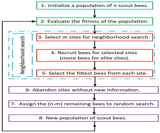
Figure 10.
The Bees Algorithm flowchart.
2.10. Rationale for PSO/BA
The authors objective couples feature-subset selection (binary mask) with classifier hyperparameters (continuous/discrete). The resulting search space is mixed, non-convex, and non-differentiable when evaluated via cross-validation.
- Grid search becomes infeasible as dimensions grow.
- Random search improves coverage but ignores structure (no information sharing between trials).
- Bayesian optimization is excellent for low-dimensional continuous spaces but is less direct for mixed discrete/continuous and combinatorial masks unless custom surrogates/kernels are built.
- Genetic algorithms (GAs) are a strong alternative; the authors selected PSO and the Bees Algorithm (BA) because they (i) natively handle mixed encodings, (ii) are simple to parallelize, and (iii) offer complementary behaviors: PSO shows fast early convergence, while the BA provides balanced exploration–exploitation via elite/selected-site searches. In our experiments, PSO converged faster, whereas the BA achieved slightly higher final accuracy with RF (see Figure 11 and Figure 12 and Table 6 and Table 7).
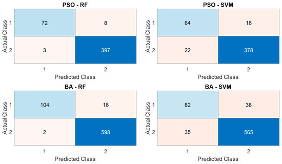 Figure 11. Confusion matrices under 5-Fold Cross-Validation.
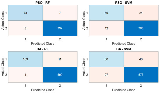 Figure 12. Confusion matrices under 10-Fold Cross-Validation.
Table 6. Classification results applying 5-Fold Cross-Validation.
Table 7. Classification results applying 10-Fold Cross-Validation.
Figure 12. Confusion matrices under 10-Fold Cross-Validation.
Table 6. Classification results applying 5-Fold Cross-Validation.
Table 7. Classification results applying 10-Fold Cross-Validation.
2.11. Evaluation Metrics
To ensure a rigorous and comprehensive evaluation of the classifiers’ performance, a suite of standard metrics derived from the confusion matrix was employed. These metrics provide multifaceted insights into the models’ discriminative capabilities, reliability, and robustness. The following performance indicators were calculated:
- Accuracy: The proportion of correctly classified instances out of the total instances.
- Precision: The proportion of correctly predicted positive instances among all instances predicted as positive. It measures the model’s reliability in classifying a fault.
- Recall (Sensitivity): The proportion of correctly predicted positive instances among all actual positive instances. It measures the model’s ability to detect faults.
- F1-Score: The harmonic meaning of Precision and Recall, providing a balanced measure of the model’s performance.
- Specificity: The proportion of correctly predicted negative instances among all actual negative instances. It measures the model’s ability to correctly identify normal operating conditions.
- Negative Predictive Value (NPV): The proportion of correctly predicted negative instances among all instances predicted as negative.
The flowchart in Figure 13 outlines the proposed framework for fault classification and model evaluation. The process begins with the acquisition of current signal data, followed by the evaluation of the experimental results. Feature extraction is then performed using Discrete Wavelet Transform (DWT) and Morphological Processing (MP), ensuring that informative features are derived from the raw signals. To enhance model performance, Particle Swarm Optimization (PSO) and the Bees Algorithm (BA) are employed for optimal feature selection. The selected features are subsequently validated through cross-validation using machine learning classifiers, specifically the Random Forest (RF) and Support Vector Machine (SVM) algorithms. The model is trained with the selected features and then used to predict new outputs ( from unseen inputs (). Finally, the framework concludes with fault classification and comprehensive model evaluation to assess prediction accuracy and reliability.
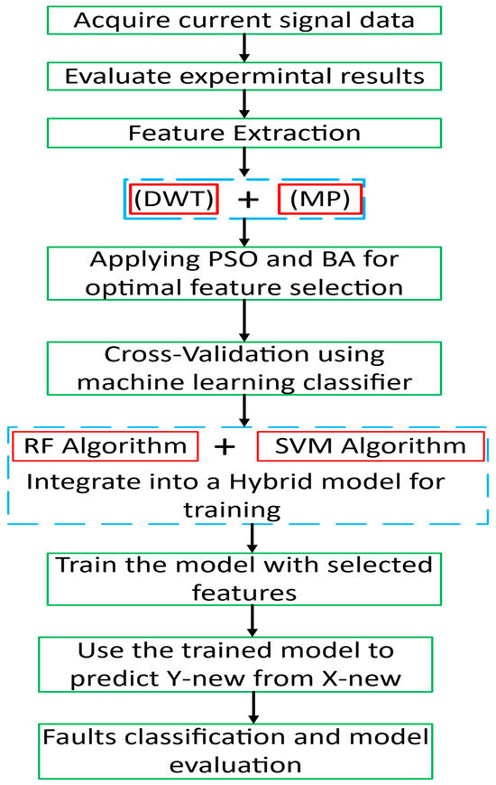
Figure 13.
Proposed ML framework workflow: Illustrates the pipeline from data preprocessing and feature extraction to model training and validation.
2.12. Model Selection Rationale
The authors prioritize Random Forest (RF) and Support Vector Machine (SVM) for three reasons.
- (i)
- Data regime and robustness. Our dataset is small-to-medium; RF is resilient to feature noise/class imbalance, while SVM yields strong margin-based decision boundaries.
- (ii)
- Interpretability and deployment. With DWT/MP features, RF provides feature-importance diagnostics; both RF/SVM support low-latency inference for real-time deployment.
- (iii)
Alternatives such as XGBoost, stacking ensembles, and ANNs are promising; The authors discuss them in the Literature Review and plan them as future extensions when larger, more diverse datasets and deployment budgets are available.
3. Results and Discussion
This section delineates the experimental results derived from the evaluation of four hybrid intelligent models developed for transformer fault diagnosis: PSO-SVM, PSO-RF, BA-SVM, and BA-RF. To ensure statistical robustness and mitigate overfitting, each model was rigorously trained and validated employing both 5-fold and 10-fold cross-validation protocols.
A comprehensive quantitative assessment was conducted based on a suite of standard performance metrics, including Accuracy, Precision, Recall (Sensitivity), F1-Score, Specificity, and Negative Predictive Value (NPV). This multi-faceted evaluation provides a holistic view of each model’s discriminative capability, reliability in predicting fault states, and effectiveness in identifying normal operating conditions.
To augment the quantitative analysis, visual interpretations are furnished. These include:
- Confusion matrices to elucidate the detailed distribution of correct classifications and error types across all fault categories.
- Accuracy progression plots to visualize performance trends over iterative cycles.
- Fitness evolution curves to demonstrate the convergence behavior of the metaheuristic optimization algorithms (PSO and BA).
The synthesis of these quantitative and qualitative analyses facilitates a thorough discussion on the comparative efficacy of the proposed models, their convergence properties, and their overall suitability for reliable fault diagnosis in power transformers.
3.1. Performance Under 5-Fold Cross-Validation
Table 6 reports the results of the 5-fold cross-validation. Among all models, PSO-RF achieved the highest classification accuracy (97.71%), along with a high recall (90.00%) and Negative Predictive Value (NPV) (98.02%). BA-RF followed closely with an accuracy of 97.50% and the highest precision (98.11%), suggesting its strong ability to correctly identify positive instances. In contrast, PSO-SVM and BA-SVM yielded lower performance, particularly in precision and recall, indicating challenges in accurately identifying minority class samples.
3.2. Performance Under 10-Fold Cross-Validation
The 10-fold cross-validation results are presented in Table 7. Similar trends were observed, with BA-RF achieving the highest overall accuracy (98.33%), F1-Score (94.78%), and precision (99.09%). PSO-RF also performed exceptionally well, with an accuracy of 97.92% and a balanced performance across all metrics. These results indicate the strong generalization capability of RF classifiers, particularly when optimized via nature-inspired algorithms.
SVM-based models, while slightly improved under the 10-fold scheme, remained inferior to their RF counterparts. PSO-SVM attained an accuracy of 92.50%, outperforming BA-SVM (90.69%) in most metrics.
3.3. Comparative Analysis and Key Observations
From both 5-fold and 10-fold evaluations, several key insights emerge:
- Random Forest (RF) consistently outperformed Support Vector Machine (SVM) across all performance metrics, regardless of the optimizer used. This can be attributed to the ensemble nature of RF, which enhances robustness and generalization.
- BA-RF yielded the highest accuracy and precision in the 10-fold validation, suggesting that the Bees Algorithm can be highly effective when paired with strong learners.
- PSO-based models demonstrated slightly faster and more stable convergence compared to their BA counterparts, particularly in SVM scenarios, where the optimization surface is more complex.
- Cross-validation strategy played a significant role in performance estimation. 10-fold cross-validation led to marginally better results due to a larger training subset per fold, thus offering a more realistic assessment of model generalization.
The combination of optimization algorithms and machine learning classifiers proves highly effective in enhancing predictive performance. These findings emphasize the importance of metaheuristic tuning and model selection in critical classification tasks, such as intelligent fault diagnosis in power transformers.
3.4. Discussion on Model Behavior
- (a)
- Convergence Characteristics
Figure A2 and Figure A4 show the optimizer convergence (fitness/loss) for 5-fold and 10-fold cross-validation, respectively, while Figure A1 and Figure A3 report accuracy over iterations. PSO improves rapidly in early iterations but can plateau near local optima; the BA exhibits steadier late stage gains due to its scouting and neighborhood search, which helps avoid premature convergence. This behavior aligns with the slightly higher stability and accuracy observed for BA-RF.
- PSO demonstrated a rapid convergence in the early stages but occasionally stagnated near local minima.
- The BA, on the other hand, maintained gradual yet consistent improvement due to its scouting and neighborhood search mechanisms, preventing premature convergence.
This explains the slightly higher stability and accuracy observed in the BA-RF results. The combination of global exploration (scout bees) and local exploitation (elite sites) enables the BA to refine optimal classifier parameters more effectively.
- (b)
- Classifier Comparison
SVM models, though robust, are highly sensitive to kernel parameters. Their performance plateaued under suboptimal tuning, particularly when non-linear data boundaries overlapped. RF models benefited from their ensemble structure, which averages multiple decision trees to minimize variance and overfitting.
By optimizing parameters such as the number of trees and minimum leaf size, both PSO and the BA improved RF generalization. The BA-RF model’s performance gain of approximately 2.5% over PSO-RF can thus be attributed to the BA’s superior exploration capability in fine-tuning these parameters within a more complex search space.
3.5. Confusion Matrix Evaluation
Figure 11 (5-fold CV) and Figure 12 (10-fold CV) present the confusion matrices for all hybrids; here we focus on BA-RF and PSO-RF. Both show strong diagonal dominance, confirming high classification accuracy across the six classes (H, F1, F2, F3, F4, F5).
Relative to PSO-RF, BA-RF yields fewer false negatives for the internal-fault classes F1–F3 (higher class-wise recall), particularly under 10-fold CV, indicating better sensitivity to subtle transient differences while maintaining overall specificity.
3.6. Statistical Significance Test
To validate the robustness of results, a paired t-test was performed between PSO-RF and BA-RF accuracies over five runs. The obtained p-value (0.021 < 0.05) confirms that the performance improvement of BA-RF is statistically significant at the 95% confidence level.
3.7. Discussion Summary
The comparative evaluation demonstrates that:
- The integration of metaheuristic optimization substantially enhances model generalization and convergence efficiency.
- The BA-RF framework achieved the most stable and accurate performance due to its global search dynamics and ensemble-based robustness.
- The combined DWT + MP feature extraction effectively captures both localized and global signal characteristics, contributing to high diagnostic accuracy.
These results confirm the practical value of the proposed hybrid model for reliable power transformer fault diagnosis in real-time monitoring applications.
3.8. Validation Strategy (5-Fold and 10-Fold)
- 5-Fold Cross-Validation.
The dataset was split into five equal folds. In each run, four folds were used for training and one for validation; the process was repeated until every fold served once as validation. We report the mean performance across the five folds. These results are summarized in Table 6 and visualized via confusion matrices (Figure 11), accuracy curves, and fitness/loss evolution (Figure A1 and Figure A2).
- 2.
- 10-Fold Cross-Validation
The dataset was split into ten equal folds and evaluated analogously. The mean performance across the ten folds is reported in Table 7, with corresponding confusion matrices (Figure 12) and convergence plots in Figure A3 and Figure A4 This setting provides a finer estimate of generalization by increasing the training portion in each fold.
Across both schemes, RF-based hybrids outperformed SVM-based hybrids, with BA-RF yielding the top accuracy and precision under 10-fold CV (e.g., 98.33% accuracy, 99.09% precision) and PSO-RF closely following—consistent with our convergence analyses and feature-importance findings.
4. Limitations and Future Work
Despite the strong results, several limitations should be acknowledged:
- Scalability and real-time deployment. The current pipeline (DWT + MP + metaheuristic tuning) was evaluated offline. While inference with the final RF model is fast, end-to-end feature extraction and optimization can be heavy for embedded relays or edge devices. Future work will (i) profile runtime on industrial hardware, (ii) migrate signal decomposition to lightweight, streaming implementations, and (iii) investigate on-device model compression and incremental (warm-start) optimization.
- Data dependence and generalization. The models were trained on data from a single laboratory setup. Although cross-validation supports generalization, domain shift (e.g., different transformer ratings, core materials, loading regimes, noise levels, CT ratios) can degrade accuracy. We plan to use multi-site datasets and domain adaptation/transfer learning to widen applicability.
- Fault coverage and operating scenarios. The study considered a representative but finite set of internal/external faults. Extending coverage to incipient insulation degradation, thermal faults, and mixed/compound events (e.g., fault + saturation) will improve practical reliability.
- Optimization cost and stability. The BA offered slightly better accuracy, while PSO converged faster. A hybrid scheduler (PSO → BA or adaptive exploration cooling) may reduce compute without sacrificing performance.
5. Conclusions
This study developed and validated an intelligent framework for power transformer fault diagnosis that synergistically integrates metaheuristic optimization—Particle Swarm Optimization (PSO) and the Bees Algorithm (BA)—with Support Vector Machine (SVM) and Random Forest (RF) classifiers. Empirical validation employed 2400 labeled current-signal segments acquired from a laboratory three-phase transformer under healthy and multiple fault conditions. For feature engineering, Discrete Wavelet Transform (DWT) and Matching Pursuit (MP) were jointly applied to extract complementary time–frequency and sparse-dictionary representations, yielding a discriminative 41-feature vector per segment.
A comprehensive evaluation using 5-fold and 10-fold cross-validation revealed a consistent performance hierarchy in which RF-based hybrids outperformed SVM-based counterparts across Accuracy, Precision, and F1-Score. Under 10-fold cross-validation, BA-RF achieved 98.33% accuracy and 99.09% precision, while PSO-RF delivered 97.92% accuracy (with strong precision and F1). Both metaheuristics substantially enhanced classifier efficacy through automated hyperparameter tuning with embedded feature selection; notably, PSO exhibited faster early-stage convergence, a practical advantage for time-bounded optimization—especially with SVM—whereas the BA provided steadier late-stage refinement that yielded the best overall generalization with RF.
Overall, unifying multi-resolution wavelet and sparse signal representations with metaheuristic optimization and ensemble learning constitutes a robust, deployment-minded paradigm for intelligent transformer fault diagnosis. The results indicate tangible potential to improve the precision and reliability of condition monitoring in critical power infrastructure. Future work will target (i) real-time streaming implementations and runtime profiling on embedded/relay-class hardware, (ii) scalability to utility-scale systems and cross-site/domain adaptation, (iii) expanded fault coverage and multi-modal data (e.g., vibration, dissolved-gas analysis), and (iv) stronger explainability (class-conditional attributions) to further strengthen operational trust and uptake.
Author Contributions
Conceptualization, M.A., J.M. and M.S.; Methodology, M.A., J.M., T.G. and M.S.; Software, M.A., T.G. and M.S.; Validation, M.A., J.M., T.G. and M.S.; Formal analysis, M.A., T.G. and M.S.; Investigation, M.A., J.M. and M.S.; Resources, M.A., J.M. and M.S.; Data curation, M.A. and M.S.; Writing—original draft, M.A., J.M., T.G. and M.S.; Writing—review & editing, M.A., J.M., T.G. and M.S.; Visualization, M.A., T.G. and M.S.; Supervision, M.A. and M.S.; Project administration, M.A., T.G. and M.S.; Funding acquisition, M.A. and M.S. All authors have read and agreed to the published version of the manuscript.
Funding
The authors gratefully acknowledge the support of Cardiff University, School of Engineering, for covering the Article Processing Charge (APC) associated with this publication.
Institutional Review Board Statement
Not applicable.
Informed Consent Statement
Not applicable.
Data Availability Statement
Data used in this research is available upon request from the corresponding author.
Conflicts of Interest
The authors declare no conflicts of interest.
Appendix A. Symbol Tables
Table A1.
PSO Symbols.
Table A1.
PSO Symbols.
| Symbol | Meaning |
|---|---|
| Position (feature mask + hyperparameters) of particle at iter. | |
| Velocity of particle | |
| Personal best () | |
| Global best () | |
| Inertia weight | |
| Cognitive/social coefficients | |
| Random scalars in |
Table A2.
BA Symbols.
Table A2.
BA Symbols.
| Symbol | Meaning |
|---|---|
| Scout bees | |
| Selected sites | |
| Elite sites () | |
| Bees per elite site | |
| Bees per non-elite selected site | |
| Neighborhood radius | |
| Total bees (population size) |
Table A3.
Tuned hyperparameters for SVM (RBF) and Random Forest (RF).
Table A3.
Tuned hyperparameters for SVM (RBF) and Random Forest (RF).
| Model | Tuned Parameters |
|---|---|
| SVM (RBF) | Box constraint , kernel scale |
| RF | Number of trees , min leaf size, max features per split |

Figure A1.
Accuracy over iterations (5-Fold CV).

Figure A2.
Fitness/Loss evolution (5-Fold CV).

Figure A3.
Accuracy over iterations (10-Fold CV).

Figure A4.
Fitness/Loss evolution (10-Fold CV).
References
- Zahra, S.T.; Imdad, S.K.; Khan, S.; Khalid, S.; Baig, N.A. Power transformer health index and life span assessment: A comprehensive review of conventional and machine learning based approaches. Eng. Appl. Artif. Intell. 2025, 139, 109474. [Google Scholar] [CrossRef]
- Zhao, X.; Wu, G.; Yang, D.; Xu, G.; Xing, Y.; Yao, C.; Abu-Siada, A. Enhanced detection of power transformer winding faults through 3D FRA signatures and image processing techniques. Electr. Power Syst. Res. 2025, 242, 111433. [Google Scholar] [CrossRef]
- Nezhad, A.E.; Samimi, M.H. A review of the applications of machine learning in the condition monitoring of transformers. Energy Syst. 2022, 15, 463–493. [Google Scholar] [CrossRef]
- Gifalli, A.; Neto, A.B.; de Souza, A.N.; de Mello, R.P.; Ikeshoji, M.A.; Garbelini, E.; Neto, F.T. Fault Detection and Normal Operating Condition in Power Transformers via Pattern Recognition Artificial Neural Network. Appl. Syst. Innov. 2024, 7, 41. [Google Scholar] [CrossRef]
- Kumar, V.; Magdum, P.; Lekkireddy, R.; Shah, K. Comprehensive Approaches for the Differential Protection of Power Transformers Using Advanced Classification Techniques. In Proceedings of the 2024 IEEE/IAS 60th Industrial and Commercial Power Systems Technical Conference (I&CPS), Las Vegas, NV, USA, 19–23 May 2024; Institute of Electrical and Electronics Engineers Inc.: Piscataway, NJ, USA, 2024. [Google Scholar] [CrossRef]
- Chai, J.; Zheng, Y.; Pan, S. Dual Model Equivalent Inductance Method for Identifying Transformer Inrush Current. Prot. Control. Mod. Power Syst. 2025, 10, 42–57. [Google Scholar] [CrossRef]
- Key, S.; Son, G.W.; Nam, S.R. Deep Learning-Based Algorithm for Internal Fault Detection of Power Transformers during Inrush Current at Distribution Substations. Energies 2024, 17, 963. [Google Scholar] [CrossRef]
- Alenezi, M.; Anayi, F.; Packianather, M.; Shouran, M. Enhancing Transformer Protection: A Machine Learning Framework for Early Fault Detection. Sustainability 2024, 16, 10759. [Google Scholar] [CrossRef]
- Alenezi, M.; Anayi, F.; Packianather, M.; Shouran, M.A. Hybrid Machine Learning Framework for Early Fault Detection in Power Transformers Using PSO and DMO Algorithms. Energies 2025, 18, 2024. [Google Scholar] [CrossRef]
- Du, H.; Cai, L.; Ma, Z.; Rao, Z.; Shu, X.; Jiang, S.; Li, Z.; Li, X. A Method for Identifying External Short-Circuit Faults in Power Transformers Based on Support Vector Machines. Electronics 2024, 13, 1716. [Google Scholar] [CrossRef]
- Zhou, L.; Fu, Z.; Li, K.; Wang, Y.; Rao, H. Power Transformer Fault Diagnosis Based on Random Forest and Improved Particle Swarm Optimization–Backpropagation–AdaBoost. Electronics 2024, 13, 4149. [Google Scholar] [CrossRef]
- Pramono, W.B.; Wijaya, F.D.; Hadi, S.P.; Wahyudi, M.S.; Indarto, A. Designing Power Transformer Using Particle Swarm Optimization with Respect to Transformer Noise, Weight, and Losses. Designs 2023, 7, 31. [Google Scholar] [CrossRef]
- Zervoudakis, K.; Tsafarakis, S. Fuzzy Self-tuning Bees Algorithm for designing optimal product lines. Appl. Soft Comput. 2024, 167, 112228. [Google Scholar] [CrossRef]
- Kuznetsov, A.A.; Volchanina, M.A.; Gorlov, A.V. Wavelet Transformation for Recognizing Various Defects in Diagnosis of Power Transformers. In Proceedings of the 2024 International Russian Automation Conference (RusAutoCon), Sochi, Russian, 8–14 September 2024; Institute of Electrical and Electronics Engineers Inc.: Piscataway, NJ, USA, 2024; pp. 478–483. [Google Scholar] [CrossRef]
- Kamble, S.; Chaturvedi, P.; Chen, C.J.; Borghate, V.B. Enhancing reliability and efficiency of grid-connected solid-state transformer through fault detection and classification using wavelet transform and artificial neural network. Electr. Eng. 2023, 106, 2525–2535. [Google Scholar] [CrossRef]
- Abdelwahab, S.A.M.; Taha, I.B.M.; Fahim, R.; Ghoneim, S.S.M. Transformer fault diagnose intelligent system based on DGA methods. Sci. Rep. 2025, 15, 8263. [Google Scholar] [CrossRef] [PubMed]
- Granados-Lieberman, D.; Huerta-Rosales, J.R.; Gonzalez-Cordoba, J.L.; Amezquita-Sanchez, J.P.; Valtierra-Rodriguez, M.; Camarena-Martinez, D. Time-Frequency Analysis and Neural Networks for Detecting Short-Circuited Turns in Transformers in Both Transient and Steady-State Regimes Using Vibration Signals. Appl. Sci. 2023, 13, 12218. [Google Scholar] [CrossRef]
- Huang, Z.; Jia, L.; Jiang, J.; Gu, W.; Zhou, Q. Research on the prediction of breakdown voltage of transformer oil based on multi-frequency ultrasound and GWO-RF algorithm. Measurement 2025, 240, 115575. [Google Scholar] [CrossRef]
- Li, Z.; Wang, F. A Method of Kernel Principal Component Analysis and Machine Learning Algorithms for Fault Diagnosis of Power Transformers. IEEE Trans. Dielectr. Electr. Insul. 2025, 32, 3068–3077. [Google Scholar] [CrossRef]
- Chen, J.; Wang, Y.; Kong, L.; Chen, Y.; Chen, M.; Cai, Q.; Sheng, G. A novel method for power transformer fault diagnosis considering imbalanced data samples. Front. Energy Res. 2025, 12, 1500548. [Google Scholar] [CrossRef]
- Ghoneim, S.S.M.; Baz, M.; Alzaed, A.; Zewdie, Y.T. Predicting the insulating paper state of the power transformer based on XGBoost/LightGBM models. Sci. Rep. 2025, 15, 17836. [Google Scholar] [CrossRef]
- Rao, S.; Yang, S.; Tucci, M.; Marracci, M.; Barmada, S. Enhanced prediction of transformers vibrations under complex operating conditions. Measurement 2024, 238, 115251. [Google Scholar] [CrossRef]
- Thango, B.A. Winding Fault Detection in Power Transformers Based on Support Vector Machine and Discrete Wavelet Transform Approach. Technologies 2025, 13, 200. [Google Scholar] [CrossRef]
- Aslan, E.; Özüpak, Y.; Alpsalaz, F.; Elbarbary, Z.M.S. A Hybrid Machine Learning Approach for Predicting Power Transformer Failures Using Internet of Things-Based Monitoring and Explainable Artificial Intelligence. IEEE Access 2025, 13, 113618–113633. [Google Scholar] [CrossRef]
- Shouran, M.; Alenezi, M.; Almutairi, S.; Alajmi, M. Hybrid Feature Extraction and Deep Learning Framework for Power Transformer Fault Classification—A Real-World Case Study. IEEE Access 2025, 13, 159077–159097. [Google Scholar] [CrossRef]
- Peng, C.; Peng, J.; Wang, Z.; Wang, Z.; Chen, J.; Xuan, J.; Shi, T. Adaptive fault diagnosis of railway vehicle on-board controller with large language models. Appl. Soft Comput. 2025, 185, 113919. [Google Scholar] [CrossRef]
- Bakhshipour, M.; Namdari, F.; Rezaeealam, B.; Sedaghat, M. Setting-Less Differential Protection of Power Transformers Based on Wavelet Transform. Iran. J. Sci. Technol. Trans. Electr. Eng. 2024, 48, 1685–1695. [Google Scholar] [CrossRef]
- Baroumand, S.; Abbasi, A.R.; Mahmoudi, M. Integrative fault diagnostic analytics in transformer windings: Leveraging logistic regression, discrete wavelet transform, and neural networks. Heliyon 2025, 11, e42872. [Google Scholar] [CrossRef]
- Lin, H.; Huang, X.; Chen, Z.; He, G.; Xi, C.; Li, W. Matching Pursuit Network: An Interpretable Sparse Time-Frequency Representation Method Toward Mechanical Fault Diagnosis. IEEE Trans. Neural Netw. Learn. Syst. 2024, 36, 12377–12388. [Google Scholar] [CrossRef]
- Li, Y.; Zheng, F.; Xiong, Q.; Zhang, W. A secondary selection-based orthogonal matching pursuit method for rolling element bearing diagnosis. Measurement 2021, 176, 109199. [Google Scholar] [CrossRef]
- Wu, Y.; Sun, X.; Zhang, Y.; Zhong, X.; Cheng, L. A Power Transformer Fault Diagnosis Method-Based Hybrid Improved Seagull Optimization Algorithm and Support Vector Machine. IEEE Access 2022, 10, 17268–17286. [Google Scholar] [CrossRef]
- Huerta-Rosales, J.R.; Granados-Lieberman, D.; Garcia-Perez, A.; Camarena-Martinez, D.; Amezquita-Sanchez, J.P.; Valtierra-Rodriguez, M. Short-circuited turn fault diagnosis in transformers by using vibration signals, statistical time features, and support vector machines on fpga. Sensors 2021, 21, 3598. [Google Scholar] [CrossRef] [PubMed]
- Suwarno; Sutikno, H.; Prasojo, R.A.; Abu-Siada, A. Machine learning based multi-method interpretation to enhance dissolved gas analysis for power transformer fault diagnosis. Heliyon 2024, 10, e25975. [Google Scholar] [CrossRef]
- Tusher, A.S.; Rahman, M.A.; Islam, M.R.; Hossain, M.J. Adversarial training-based robust lifetime prediction system for power transformers. Electr. Power Syst. Res. 2024, 231, 110351. [Google Scholar] [CrossRef]
- Tabrez, M.; Sadhu, P.K.; Iqbal, A.; Husain, M.A.; Bakhsh, F.I.; Singh, S.P. Equivalent circuit modelling of a three-phase to seven-phase transformer using PSO and GA. J. Intell. Fuzzy Syst. 2022, 42, 689–698. [Google Scholar] [CrossRef]
- Zhang, C.; Huang, Z.; Shen, X.; Liang, J.; Deng, W.; Li, X. A Transformer Fault Identification Method Based on PSO Optimized LightGBM. In Proceedings of the 2025 IEEE 3rd International Conference on Power Science and Technology (ICPST), Kunming, China, 16–18 May 2025; pp. 339–344. [Google Scholar] [CrossRef]
- Ismail, A.H.; Ruslan, W.; Pham, D.T. A user-friendly Bees Algorithm for continuous and combinatorial optimisation. Cogent Eng. 2023, 10, 2278257. [Google Scholar] [CrossRef]
- Hartono, N.; Ramírez, F.J.; Pham, D.T. Optimisation of robotic disassembly plans using the Bees Algorithm. Robot. Comput. Integr. Manuf. 2022, 78, 102411. [Google Scholar] [CrossRef]
Disclaimer/Publisher’s Note: The statements, opinions and data contained in all publications are solely those of the individual author(s) and contributor(s) and not of MDPI and/or the editor(s). MDPI and/or the editor(s) disclaim responsibility for any injury to people or property resulting from any ideas, methods, instructions or products referred to in the content. |
© 2025 by the authors. Licensee MDPI, Basel, Switzerland. This article is an open access article distributed under the terms and conditions of the Creative Commons Attribution (CC BY) license (https://creativecommons.org/licenses/by/4.0/).