A Prediction Method for the Surface Arc Inception Voltage of Epoxy Resin Based on an Electric Field Feature Set and GS-SVR

Abstract

To address the critical challenges posed by the complex coastal climate on the external insulation of electrical equipment, research into the prediction of the surface arc inception voltage of epoxy resin under multiple conditions is of great significance for preventing failures and guiding operations and maintenance. In this regard, we propose a prediction method for surface arc inception voltage based on grid search-optimized support vector regression (GS-SVR). Using a 21-dimensional electric field feature set along the shortest inter-electrode path as model input, high-accuracy prediction of surface arc inception voltage under complex conditions is achieved. The results demonstrate that the model accurately predicts surface arc inception voltage with limited samples, achieving a mean absolute percentage error (MAPE) of 6.24%. Furthermore, the non-uniform coefficient-based dataset partitioning method improves prediction accuracy compared to random partitioning, with the lowest MAPE of only 2.39%. The findings provide theoretical and technical support for improving the anti-pollution flashover and anti-condensation performance of epoxy resin insulating materials.

1. Introduction

With the advancement of the “dual-carbon” strategic goals, future power systems are expected to exhibit new characteristics. Renewable energy will be integrated on a large scale in a distributed manner, with various energy sources operating synergistically and under coordinated regulation [1,2]. Against this backdrop, power systems are gradually transitioning to a new structure dominated by clean energy. Active development of renewable sources such as solar and offshore wind power will become an important direction [3,4,5]. However, the southeastern coastal regions of China, characterized by a humid, hot, and saline-rich climate, impose extremely high demands on the insulation reliability of electrical equipment [6].

Surface flashover caused by creeping discharge is a major form of insulation failure on the surface of electrical equipment [7,8]. In environments with high humidity and heavy contamination, such as rain, fog, dew, and haze, a wet polluted layer forms on the surface of insulation materials after moisture absorption, significantly reducing the insulation margin of electrical equipment. Flashover may even occur under operating voltage, seriously threatening the reliable operation of the power system [9,10,11,12]. Research on predictive models for the surface arc inception voltage of insulating materials in complex environments is therefore of great significance for the operational stability of power systems.

As research on discharge mechanisms continues to deepen, scholars worldwide have continuously summarized, generalized, and revised a series of classical empirical discharge formulas based on extensive experimental data [13,14]. In addition, numerous researchers have determined the physical parameters and characteristics of discharge through experiments, attempting to achieve accurate prediction of discharge behavior from a physical mechanism perspective [15,16,17].

With the continuous advancement of artificial intelligence algorithms, researchers have applied them to the study of discharge characteristic prediction models, with promising results [18], enabling data-driven approaches for predicting discharge behavior. For instance, Mokhnache et al. proposed a breakdown voltage prediction method based on neural networks for point–barrier–plane structures [19]. Shakeel Akram et al. developed a deep learning-based model to predict the inception discharge voltage of insulation in electric vehicles [20]. Qiu et al. introduced a method combining electric field simulation, feature extraction, and machine learning algorithms to predict switching impulse discharge voltage in ultra-high-voltage transmission line-tower air gaps [21].

Support vector machines also have certain applications in the high-voltage field [22,23,24,25]. For instance, Dai proposed an improved SVR model based on WOA optimization, achieving high-precision prediction of pre-insertion resistance temperature, Kim used the SVR algorithm to predict impulse impact voltage, and Qiu applied the SVR model to predict lightning impulse flashover voltage.

In summary, although certain achievements have been made in recent years in the modeling of surface discharge of insulating materials, researchers rarely address flashover voltage prediction under complex environmental conditions. Moreover, data-driven methods generally require large sample sizes, obtaining raw experimental discharge data remains challenging, and sample availability is limited—issues that have not been thoroughly investigated. There is currently a lack of predictive models for the arc inception voltage of insulating materials that can be effectively applied in practical engineering. To address these limitations, in this study, we focus on epoxy resin materials and propose a surface arc inception voltage prediction model based on support vector regression (SVR) optimized with grid search (GS). An optimized sample partitioning method using the electric field non-uniformity coefficient is introduced to enhance model performance.

2. Methods

2.1. Definition of the Electric Field Feature Set

The surface electric field distribution of insulating materials significantly influences the surface flashover voltage. To comprehensively characterize the electric field distribution over the epoxy resin surface, a 21-dimensional set of electric field features is therefore defined from four aspects: electric field intensity, electric field non-uniformity, integral of electric field intensity, and path length. These aspects constitute the electric field feature set, as shown in Table 1.

Table 1. Electric Field Characteristic Quantities.

Category	Electric Field Characteristic Quantity	Amount
Electric field intensity	Maximum value Emax, Minimum value Emin, Average value Eave	3
Electric field non-uniformity	Variance Evar, Standard deviation Estd, Field strength distortion rate Ed, Range R, Range coefficient Cr, Standard deviation Cv, Maximum value/Average value Eha, Minimum value/Average value Ela	8
Electric field intensity integral	The integral of the square of the electric field strength Ss, Value of expectation Ssa, Integration of the voltage electrode from its maximum value to its minimum value Sh, Integration of the voltage electrode from the minimum value Sl, The integral of the field strength exceeding 75% of Emax region S75%, The integral of the field strength exceeding 90% of Emax region S90%	6
Path length	The path length in the region where the field strength exceeds 75% of Emax L75%, The path length in the region where the field strength exceeds 90% of Emax L90%, The path from the high-voltage electrode to the point of minimum electric field intensity Lh, Full width at half maximum Lf	4

The electric field intensity category reflects the magnitude of the electric field in the discharge gap, which is related to the initiation of surface discharge. The electric field non-uniformity category represents the overall uniformity of the field distribution in the discharge gap, affecting both the initiation and pattern of surface discharge, thereby influencing the flashover voltage. The integral of electric field intensity reflects the electric field energy. Since the surface discharge process can be regarded as an energy release process, energy is a key factor influencing the flashover voltage. The path length category supplements the electric field non-uniformity features by characterizing local non-uniformities in the electric field distribution.

2.1.1. Electric Field Intensity Group

The differential form expression of the system of equations is as follows: The electric field intensity category mainly includes maximum value E_max, minimum value E_min, and average value E_ave. The formula for its calculation is as follows:

$$E_{\min }=\min \left\{E_i\right\},i=1,2,\cdots ,n$$

(1)

$$E_{\max }=\max \left\{E_i\right\},i=1,2,\cdots ,n$$

(2)

$$E_{\mathrm{ave}}={\displaystyle \frac{1}{n}}{\displaystyle \sum _{i=1}^n{E}_i}$$

(3)

In the formula, E_i represents the electric field intensity at the i-th point on the shortest path, and n is the number of data points representing the electric field intensities of each sample.

2.1.2. Electric Field Non-Uniformity Group

The electric field non-uniformity category mainly includes variance E_var, standard deviation E_std, field strength distortion rate E_d, range R, range coefficient C_r, standard deviation C_v, maximum value/average value E_ha, and minimum value/average value E_la. The formula for its calculation is as follows:

$$E_{\mathrm{var}}={\displaystyle \frac{1}{n}}{\displaystyle \sum _{i=1}^n{\left(E_i-E_{\mathrm{ave}}\right)}^2}$$

(4)

$$E_{\mathrm{std}}=\sqrt{{\displaystyle \frac{1}{n}}{\displaystyle \sum _{i=1}^n{\left(E_i-E_{\mathrm{ave}}\right)}^2}}$$

(5)

$$E_{\mathrm{d}}={\displaystyle \frac{E_{\max }-E_{\mathrm{ave}}}{E_{\mathrm{ave}}}}$$

(6)

$$R=E_{\max }-E_{\min }$$

(7)

$$C_{\mathrm{r}}={\displaystyle \frac{R}{E_{\mathrm{ave}}}}$$

(8)

$$C_{\mathrm{v}}={\displaystyle \frac{E_{\mathrm{std}}}{E_{\mathrm{ave}}}}$$

(9)

$$E_{\mathrm{ha}}={\displaystyle \frac{E_{\max }}{E_{\mathrm{ave}}}}$$

(10)

$$E_{\mathrm{la}}={\displaystyle \frac{E_{\min }}{E_{\mathrm{ave}}}}$$

(11)

2.1.3. Electric Field Intensity Integral Group

The electric field intensity integral mainly includes the integral of the square of the electric field strength S_s, the value of expectation S_sa, the integration of the voltage electrode from its maximum value to its minimum value S_h, the integration of the voltage electrode from the minimum value S_l, the integral of the field strength exceeding 75% of E_max region S_75%, and the integral of the field strength exceeding 90% of E_max region S_90%. The formula for its calculation is as follows:

$$S_{\mathrm{s}}={\displaystyle {\int }_0^3{E}^2}dl$$

(12)

$$S_{\mathrm{sa}}\approx {\displaystyle \frac{1}{n}}{\displaystyle \sum _{i=1}^n{E_i}^2}$$

(13)

$$S_{\mathrm{h}}={\displaystyle {\int }_0^{d}E}dl$$

(14)

$$S_{\mathrm{l}}={\displaystyle {\int }_d^{3}E}dl$$

(15)

$$S_{75\%}={\displaystyle \underset{E_i>75\%E_{\max }}{\int }{E}_{i}dl}$$

(16)

$$S_{90\%}={\displaystyle \underset{E_i>90\%E_{\max }}{\int }{E}_{i}dl}$$

(17)

In the formula, d represents the path length from the high-voltage electrode to the point of minimum electric field intensity, measured in centimeters.

2.1.4. Path Length Group

Path length mainly includes the path length in the region where the field strength exceeds 75% of E_max L_75%, the path length in the region where the field strength exceeds 90% of E_max L_90%, the path from the high-voltage electrode to the point of minimum electric field intensity L_h, and the full width at half maximum L_f. In this context, the half-peak full width L_f refers to the width of the peak at 50% of the maximum electric field intensity. The formula for its calculation is as follows:

$$L_{75\%}={\displaystyle \sum _{j=1}^m{d}_j}$$

(18)

$$L_{90\%}={\displaystyle \sum _{j=1}^g{d}_j}$$

(19)

$$L_{\mathrm{h}}=d$$

(20)

In the formula, m represents the number of sampling points where the electric field intensity is greater than 75% of E_max, and g represents the number of sampling points where the electric field intensity is greater than 90% of E_max.

2.2. Sample Division Method Based on the Coefficient of Electric Field Non-Uniformity

Reasonable selection of training samples can improve the accuracy of the predictive model. The surface arc inception voltage is significantly influenced by the degree of electric field non-uniformity. The electric field non-uniformity coefficient can effectively represent the inhomogeneity of the electric field across various structures. Therefore, an optimized classification of training samples was performed based on the non-uniformity coefficient method.

The electric field non-uniformity coefficient f is defined as the ratio of the maximum electric field strength to the average electric field strength, given by the following formula:

$$f={\displaystyle \frac{E_{\max }}{E_{\mathrm{ave}}}}$$

(21)

The optimization process for selecting training samples based on the electric field non-uniformity coefficient consists of the following two steps:

(1)

The electric field non-uniformity coefficient is calculated for all electric field sample data along the shortest path. Based on the results, several intervals of the coefficient are defined. All samples are categorized into their respective intervals, and the number of samples in each interval is counted.

(2)

Based on the sample count in each interval, training samples are randomly selected in a proportional manner. During the selection process, samples are drawn as evenly as possible from each interval.

2.3. SVR Algorithm Based on GS Optimization

Support vector machine (SVM), a machine learning method, was first proposed by Vapnik in 1995. This approach remains effective for handling nonlinear models even with small sample sizes and demonstrates strong generalization capabilities. Support vector regression (SVR) is primarily used to solve regression problems, where the output is continuous. Given the challenges in obtaining raw discharge experimental data and the limited sample availability, in this study, we employed SVR to establish a multidimensional nonlinear relationship between the surface arc inception voltage and the electric field feature set along the shortest path.

The predictive performance of the SVR model is mainly determined by its decision function, whose key parameters include the penalty coefficient c and the kernel function parameter γ. To obtain a relatively optimal parameter combination (c,γ), a grid search (GS) algorithm combined with K-fold cross-validation was used for hyperparameter optimization.

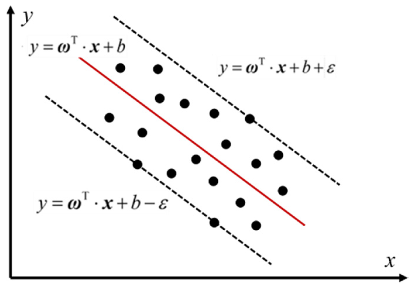
As shown in Figure 1, let the sample set be defined as (x_i, y_i), where i = 1, 2, …, N, with x_i ∈ R^N and y_i ∈ R. SVR characterizes the multidimensional nonlinear relationship between the input vector x and the output y through a hyperplane, expressed as f(x) = ωx + b, where ω ∈ R^N and b ∈ R. The hyperplane f(x) must satisfy the insensitive loss constraint:

$$\left|y_i-f({\mathit{x}}_i)\right|\le \epsilon , i=1,2,\cdots ,N$$

(22)

Figure 1. Schematic diagram of the principle of support vector regression machine.

In the formula, x_i represents the i-th input vector, y_i represents the i-th output parameter of the training set, and ɛ is the insensitive loss coefficient.

The distance d_i from any sample (x_i, y_i) to the hyperplane is as follows:

$$d_i={\displaystyle \frac{\left|\mathit{\omega }·{\mathit{x}}_i+b-y_i\right|}{\sqrt{1+{‖\mathit{\omega }‖}^2}}}\le {\displaystyle \frac{\epsilon }{\sqrt{1+{‖\mathit{\omega }‖}^2}}}, i=1,2,\cdots ,N$$

(23)

In the model solution, the main focus is on the solution of the optimal hyperplane. If this hyperplane satisfies that the distance from the training sample set to the hyperplane is the smallest, then it can be considered the optimal hyperplane. The solution to the problem of the optimal hyperplane is as follows:

$$\left\{\begin{array}{l}\min \phi (\mathit{\omega })={\displaystyle \frac{1}{2}}{‖\mathit{\omega }‖}^2\\ \mathrm{s}.\mathrm{t}. \left|\mathit{\omega }·{\mathit{x}}_i+b-y_i\right|\le \epsilon , i=1,2,\cdots ,N\end{array}\right.$$

(24)

Introduce the relaxation variable ξ and optimize it:

$$\left\{\begin{array}{l}\min \phi (\mathit{\omega })={\displaystyle \frac{1}{2}}{‖\mathit{\omega }‖}^2+C{\displaystyle \sum _{i=1}^n\left({\xi }_i+{{\xi }_i}^{\ast }\right)}\\ \mathrm{s}.\mathrm{t}. f({\mathit{x}}_i)-y_i\le {{\xi }_i}^{\ast }+\epsilon , y_i-f({\mathit{x}}_i)\le {\xi }_i+\epsilon , {\xi }_i,{{\xi }_i}^{\ast }\ge 0, i=1,2,\cdots ,n\end{array}\right.$$

(25)

To simplify the solution in the high-dimensional space, by introducing Lagrange multipliers α_i and α_i^*, the original problem is transformed into a dual problem:

$$\left\{\begin{array}{l}L={\displaystyle \frac{1}{2}}{‖\mathit{\omega }‖}^2+C{\displaystyle \sum _{i=1}^n\left({\xi }_i+{{\xi }_i}^{\ast }\right)}-{\displaystyle \sum _{i=1}^n{\alpha }_i\left[{\xi }_i+\epsilon -y_i+\mathit{w}·{\mathit{x}}_i+b\right]}\\ -{\displaystyle \sum _{i=1}^n{{\alpha }_i}^{\ast }\left[{\xi }_i+\epsilon -y_i-\mathit{w}·{\mathit{x}}_i-b\right]}-{\displaystyle \sum _{i=1}^n{\mu }_i\left({\xi }_i+{{\xi }_i}^{\ast }\right)}\\ \mathrm{s}.\mathrm{t}. {\alpha }_i, {{\alpha }_i}^{\ast }, {\mu }_i\ge 0, i=1,2,\cdots ,n\end{array}\right.$$

(26)

In the formula, C is the penalty coefficient.

During the solution process, the nonlinear regression problem in the high-dimensional space must be addressed. A kernel function can be introduced to map it to the high-dimensional space for the regression solution. The optimization problem can be expressed in the equivalent dual form as follows:

$$\left\{\begin{array}{l}\max W(\alpha ,{\alpha }^{\ast })={\displaystyle \frac{1}{2}}{\displaystyle \sum _{i=1}^n\left({\alpha }_i-{{\alpha }_i}^{\ast }\right)\left({\alpha }_j-{{\alpha }_j}^{\ast }\right)K({\mathit{x}}_i·{\mathit{x}}_j)}\\ +{\displaystyle \sum _{i=1}^n\left({\alpha }_i-{{\alpha }_i}^{\ast }\right)y_i}-{\displaystyle \sum _{i=1}^n\left({\alpha }_i+{{\alpha }_i}^{\ast }\right)\epsilon }\\ \mathrm{s}.\mathrm{t}. {\displaystyle \sum _{i=1}^n\left({\alpha }_i-{{\alpha }_i}^{\ast }\right)}=0, 0\le {\alpha }_i,{{\alpha }_i}^{\ast }\le C, i=1,2,\cdots ,n\end{array}\right.$$

(27)

The expression K(x_i, x_j) = φ(x_i)^Tφ(x_j) represents the kernel function. When solving the optimal problem using this expression, the radial basis kernel function is commonly used in SVR, and the expression is as follows:

$$K({\mathit{x}}_i,{\mathit{x}}_j)=\exp (-\gamma {‖{\mathit{x}}_i-{\mathit{x}}_j‖}^2),\gamma >0$$

(28)

In the formula, γ is the parameter of the kernel function.

After solving the above formula, it can be determined that the support vectors should be the samples corresponding to the cases where α_i or α_i^* is not zero, and they should satisfy:

$$\left\{\begin{array}{l}{\alpha }_i\left[{\xi }_i+\epsilon -y_i+f({\mathit{x}}_i)\right]=0, i=1,2,\cdots ,n\\ {{\alpha }_i}^{\ast }\left[{\xi }_i+\epsilon -y_i+f({\mathit{x}}_i)\right]=0, i=1,2,\cdots ,n\\ \left(C-{\alpha }_i\right){\xi }_i=0, i=1,2,\cdots ,n\\ \left(C-{{\alpha }_i}^{\ast }\right){\xi }_i=0, i=1,2,\cdots ,n\end{array}\right.$$

(29)

Based on the above equations, the final expression for the optimal hyperplane can be obtained:

$$f(x)={\displaystyle \sum _{i=1}^N\left({\alpha }_i-{{\alpha }_i}^{\ast }\right)}K({\mathit{x}}_i,\mathit{x})+b$$

(30)

Cross-validation is a widely used optimization method in machine learning for building models, particularly in scenarios with limited sample availability. It effectively helps prevent issues such as overfitting and underfitting. The total samples are divided into K mutually exclusive subsets. In each iteration, K-1 subsets are used as the training set, and the remaining subset is used as the validation set. This process forms different training and validation set combinations for model training. After K rounds of cross-validation, every subset has been used exactly once as the validation set, making the final trained model more robust and reliable.

During the cross-validation process, the grid search algorithm is further employed to automate parameter optimization. Grid search is an exhaustive hyperparameter tuning method that predefines the value ranges and step sizes for each hyperparameter. It systematically traverses all possible parameter combinations and selects the optimal one based on performance on the validation set. This approach ensures a comprehensive exploration of the parameter space, providing the model with a globally optimal hyperparameter configuration.

2.4. Error Analysis Method

In this study, three error metrics—root mean square error (RMSE), mean absolute percentage error (MAPE), and mean square percentage error (MSPE)—were employed to comprehensively evaluate the prediction results.

(1)

RMSE: The influence of large errors is amplified through the squared term, making RMSE highly sensitive to outliers or significant deviations in the prediction results. This metric is particularly responsive to the distribution of prediction errors and is commonly employed to evaluate both the overall prediction accuracy and the stability of the model. The expression is given as follows:

$$RMSE=\sqrt{{\displaystyle \frac{1}{n}}{\displaystyle \sum _{i=1}^n{\left(U_t-U_p\right)}^2}}$$

(31)

(2)

MAPE: Prediction deviation is expressed in the form of relative error, which eliminates the influence of data dimension and facilitates comparison across datasets with different scales or magnitudes. It is particularly suitable for evaluating the average prediction accuracy of the model at an overall level. The expression is given as follows:

$$MAPE={\displaystyle \frac{1}{n}}{\displaystyle \sum _{i=1}^n\left|\frac{U_t-U_p}{U_t}\right|}$$

(32)

(3)

MSPE: A square operation is introduced based on MAPE, thereby assigning greater penalty weights to larger relative errors. This metric can effectively identify extreme relative errors in the model and is suitable for evaluating the uniformity and reliability of the prediction result distribution. The expression is given as follows:

$$MSPE={\displaystyle \frac{1}{n}}\sqrt{{\displaystyle \sum _{i=1}^n{\left(\frac{U_t-U_p}{U_t}\right)}^2}}$$

(33)

In the formula, U_t and U_p represent the test value and the predicted value of the arc inception voltage, and n is the number of samples.

2.5. Arc Inception Voltage Prediction Process

In this study, we introduced the grid search parameter optimization algorithm into the support vector regression machine and established the GS-SVR model for predicting the surface arc inception voltage. The main process of the prediction model is shown in Figure 2. The specific workflow is as follows:

Figure 2. Workflow of the arc inception voltage prediction model based on GS-SVR.

(1)

Tests were conducted to measure original surface arc inception voltage samples under different environmental conditions. A simulation model of the electric field distribution for surface arc initiation was established based on experimental parameters. The electric field distribution data along the shortest path were obtained, and a 21-dimensional electric field feature set was defined and extracted to form the original feature dataset.

(2)

The original electric field feature set was max–min normalized. The dataset was then divided into training and testing sets using both random partitioning and the non-uniformity coefficient method.

(3)

Before model training, the grid search (GS) algorithm was applied to optimize the key hyperparameters (c,γ). The optimal hyperparameter combination was subsequently used in the GS-SVR prediction model for surface arc inception voltage.

(4)

The GS-SVR model was used to predict the arc inception voltage of the test samples. The predicted values were compared with experimental results, and error metrics were analyzed to evaluate prediction performance.

3. Experimental Verification

3.1. Discharge Test Setup

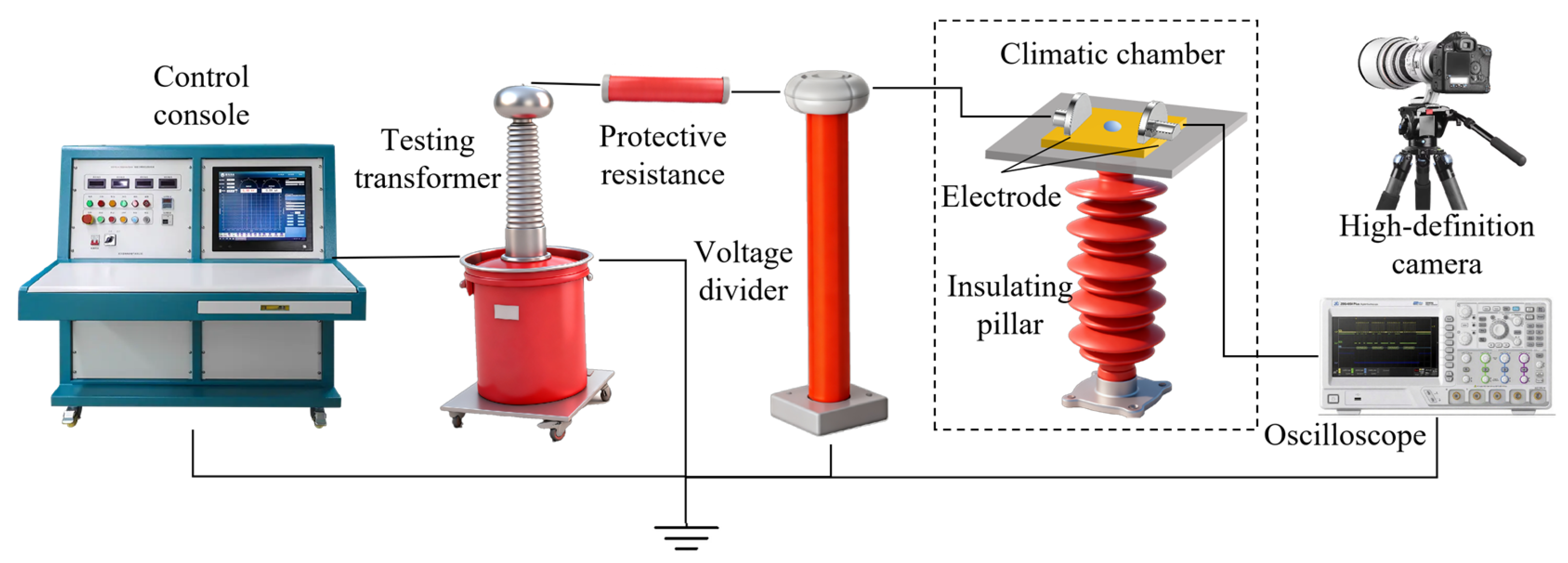
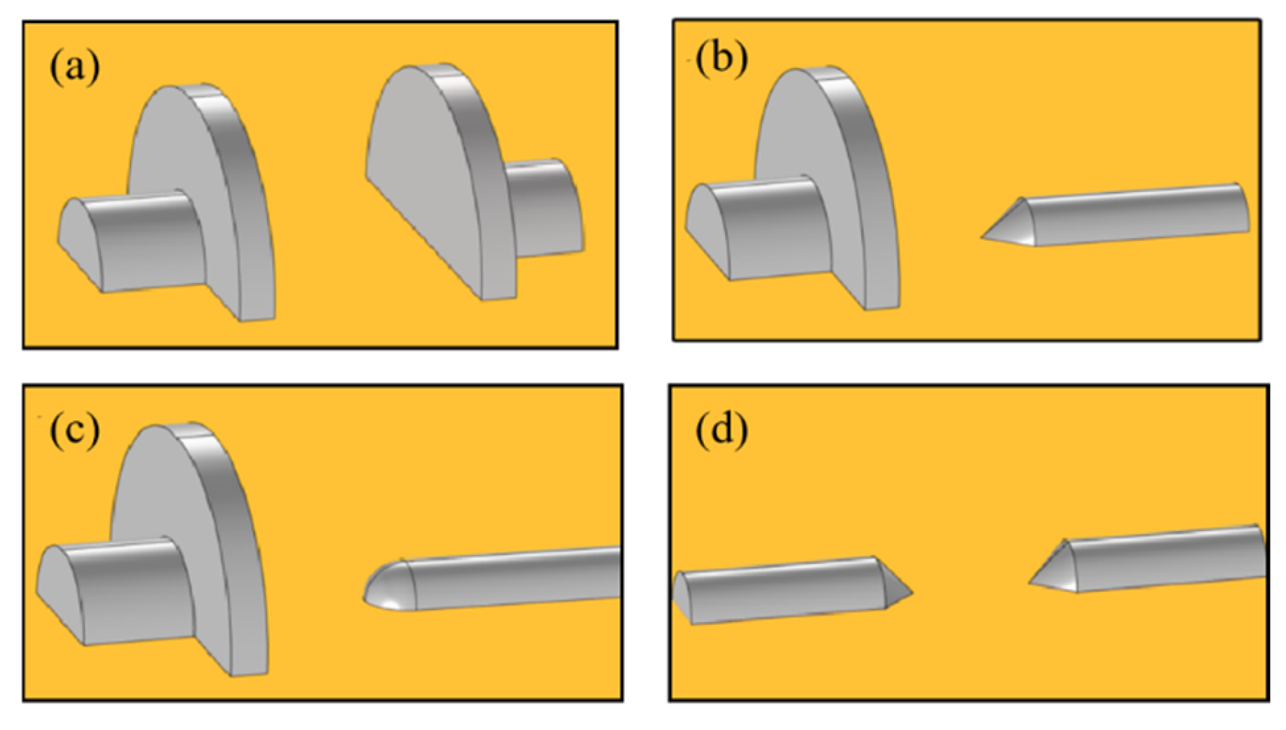
The discharge test platform is shown in Figure 3. It is mainly composed of an AC voltage generator, a voltage divider, test electrodes, a non-inductive resistor, and a measurement system. The AC test power supply (YDJ-5 kVA/100 kV) operates at a frequency of 50 Hz. A water resistor of 5 kΩ is used as the current-limiting resistor. The ratio of the capacitor voltage divider is 1000:1. The test electrodes are composed of 304 stainless steel, and electrodes of three different shapes (plate, rod, and needle) are used in four different configurations. A detailed schematic is shown in Figure 4.

Figure 3. Schematic Diagram of Discharge Test Equipment.

Figure 4. Schematic diagram of the test electrode combination: (a) plate electrode–plate electrode; (b) plate electrode–needle electrode; (c) plate electrode–rod electrode; (d) needle electrode–needle electrode.

The arc inception voltage U was selected as the experimental indicator. The influencing factors included ambient temperature, temperature difference between the environment and the insulation material surface, relative humidity, air velocity, electrode shape, number of droplets, and contamination composition. Each factor was tested at four levels. The specific values are presented in Table 2, where T, ΔT, RH, and S denote ambient temperature, temperature difference, relative humidity, air velocity, and the number of droplets, respectively. ESDD and NSDD represent the equivalent salt deposit density and the non-soluble salt deposit density, respectively.

Table 2. Experimental Variables and Expected Parameter Settings.

NO.	T (°C)	ΔT (°C)	RH (%)	S (m/s)	Electrode Shape	Number of Droplets	Contaminant (mg/cm2)
							ESDD	NSDD
1	25	10	75	0	Plate–plate	0	0.05	0.5
2	20	5	65	1	Rod–plate	2	0.10	1.0
3	30	15	85	2	Needle–plate	4	0.20	1.5
4	35	20	95	3	Needle–needle	6	0.30	2.5

The experimental procedure for surface discharge testing of epoxy resin under multi-factor conditions is as follows:

First, epoxy resin samples measuring 100 mm × 100 mm were prepared and then cleaned with alcohol and dried using air blowing. For samples requiring contamination, an artificial contamination solution was prepared according to the ESDD and NSDD values listed in Table 2, following the solid-layer method described in GB/T 4585-2024 [26]. The contaminated samples were produced using a brushing method.

Thereafter, the climatic conditions inside the environmental chamber were adjusted based on the values presented in Table 2 to achieve the target values of temperature, temperature difference, relative humidity, and air velocity. The conditions were stabilized for 10 min.

Lastly, the discharge test was carried out on the test platform. A uniform boosting method was applied, with the voltage initially rising at a rate of 1 kV/s. After reaching 80% of the expected arc inception voltage, the voltage was increased at a rate of 5% of the expected value per second until flashover occurred. The entire process was recorded using a high-speed camera, and the arc inception voltage value was documented.

3.2. Experimental Results

Based on the above epoxy resin surface discharge test, 28 sets of arc inception voltage data under different conditions were obtained, as shown in Table 3. Among them, the standard group was set at a temperature of 25 °C, a temperature difference of 10 °C, a wind speed of 0 m/s, and a relative humidity of 75%. To ensure the reliability of the results, each group of experiments was conducted three times, and the average value of the arc inception voltages was ultimately taken.

Table 3. Arc Inception Voltage of Test Samples.

No.	Variate	Parameter	Arc Inception Voltage (kV)
1	Temperature (°C)	20	13.4
2		25	15.8
3		30	16.8
4		35	16.5
5	Temperature difference (°C)	5	17.3
-		10	-
6		15	14.0
7		20	12.2
-	Air velocity (m/s)	0	-
8		1	12.8
9		2	12.0
10		3	10.5
11	Relative humidity (%)	65	17.4
-		75	-
12		85	16.0
13		95	13.2
14	Electrode shape	Plate–plate	15.8
15		Plate–rod	15.1
16		Plate–needle	15.0
17		Needle–needle	14.1
18	Number of droplets	0	16.2
-		2	-
19		4	14.7
20		6	14.0
21	Dry contamination (mg/mL)	5	15.5
22		10	15.2
23		15	13.8
24		20	12.8
25	Wet contamination (mg/mL)	5	2.07
26		10	1.30
27		15	0.86
28		20	0.41

Different environmental variables can lead to variations in the arc initiation voltage. Taking temperature, humidity, and contamination level as examples, a brief analysis is conducted to explain the factors responsible for the changes in the arc initiation voltage.

An increase in environmental temperature will cause the environmental dew point temperature to rise. Under the same temperature difference, it will be more difficult for condensation to form on the material surface, and even if condensation does occur, the droplet radius will be smaller. This factor will reduce the likelihood of conductive channel formation, thereby increasing the arc initiation voltage.

When the relative humidity increases, water vapor is more likely to condense into large droplets on the epoxy resin surface. These droplets show a tendency to connect to form local conductive paths, resulting in a decrease in the arc initiation voltage.

When the degree of contamination increases, the contaminant particles attached to the material surface will absorb moisture to form a large-area continuous water film. Concurrently, the soluble components in the contaminants will significantly increase the surface conductivity, and both of these factors jointly promote the formation of conductive paths, resulting in a decrease in the arc initiation voltage.

3.3. Electric Field Feature Set Extraction and Sample Division

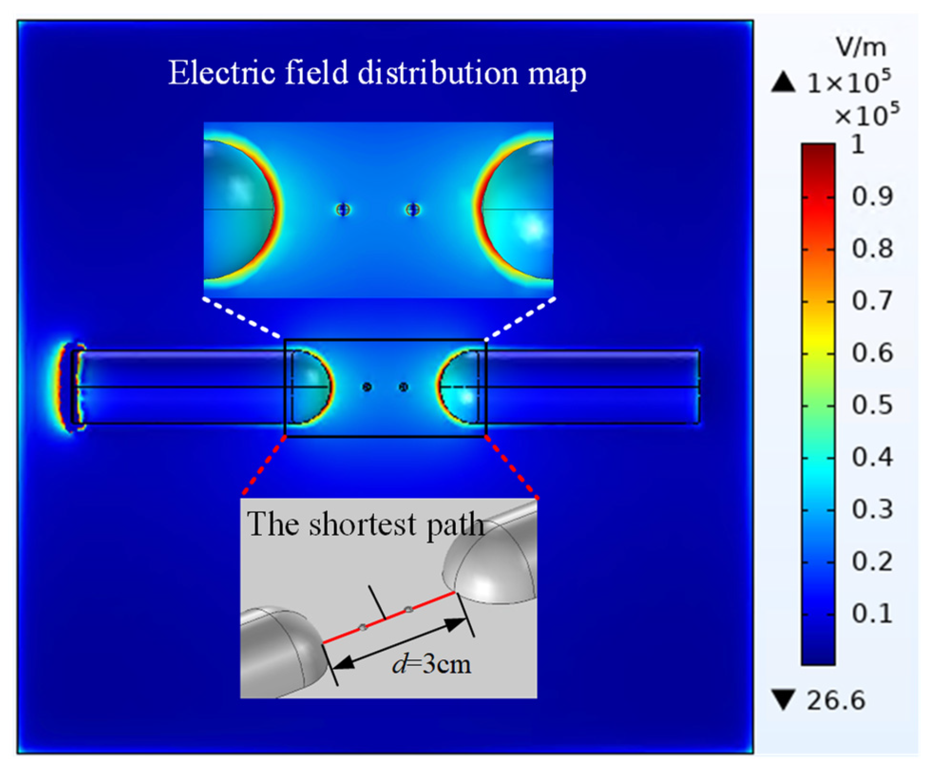
Based on the environmental variables presented in Table 3, a multi-physics field coupling simulation model was established, and the electric field distribution dataset along the shortest path under different temperatures, relative humidities, and other variables was calculated. Taking the sample with an environmental temperature of 25 °C, a temperature difference of 10 degrees Celsius, and a relative humidity of 75% as an example, the corresponding electric field distribution map is shown in Figure 5. In this figure, the length of the shortest path is 3 cm.

Figure 5. Cloud diagram of the electric field distribution in the discharge model and schematic diagram of the shortest path.

Taking the dry contamination test group as an example, the electric field data along the shortest path between electrodes under contaminant concentrations ranging from 5 mg/mL to 20 mg/mL are shown in Figure 6. It can be observed that the electric field strength reaches its maximum near the high-voltage and low-voltage electrodes. As the distance increases from the electrodes toward the center, the electric field strength gradually decreases, resulting in an overall U-shaped distribution. After computing the electric field distribution, the electric field data along the shortest inter-electrode path can be extracted. The 21-dimensional electric field feature set is then derived using Equations (1)–(20).

Figure 6. Electric field distribution under different levels of contamination.

3.4. Sample Division

By calculating the electric field non-uniformity coefficient of the test samples and considering the sample quantities within each interval range, with a step size of 3 for the non-uniformity coefficient, the total test samples were divided into four different intervals, as shown in Table 4. It can be seen that the sample numbers within each interval are evenly distributed. Among them, the samples in the interval of 3 to 6 represent the lowest number; however, 17.9% of the samples still fall within this range.

Table 4. The results of the test samples classified according to the coefficient of non-uniformity.

Unevenness Coefficient Range	Sample Number	Total Sample Quantity
1.0~3.0	21, 22, 23, 24, 25, 26, 27, 28	8
3.0~6.0	3, 4, 5, 11, 18	5
6.0~9.0	2, 6, 12, 14, 15, 16, 19, 20	8
>9.0	1, 7, 8, 9, 10, 13, 17	7

Given a total of 28 original samples, the ratio of training samples to test samples was set to 6:1 in this study. Two methods were used to partition the training and test samples: random partitioning and non-uniformity coefficient-based partitioning.

Following the random partitioning method, 24 training samples and 4 test samples were randomly selected from the 28 samples listed in Table 3. In the non-uniformity coefficient-based method, one sample was randomly chosen from each of the four non-uniformity intervals shown in Table 4 to form the test set, with the remaining 24 samples used as the training set.

Two separate partitioning trials were conducted using each method. The results are summarized in Table 5. Sample Sets 1 and 2 correspond to the random partitioning method, while Sample Sets 3 and 4 were obtained through non-uniformity coefficient-based partitioning with random selection within each interval.

Table 5. The result of the division between training samples and test samples.

Sample Set Number	Training Sample Number	Test Sample Number
1	1, 2, 3, 4, 5, 6, 7, 8, 10, 11, 12, 13, 15, 16, 17, 18, 19, 20, 21, 23, 24, 25, 27, 28	9, 14, 22, 26
2	1, 2, 3, 4, 5, 6, 7, 8, 9, 10, 11, 12, 13, 15, 17, 18, 19, 21, 23, 24, 25, 26, 27, 28	14, 16, 20, 22
3	1, 3, 4, 6, 7, 9, 10, 11, 12, 13, 14, 15, 16, 17, 18, 19, 20, 21, 22, 23, 24, 25, 27, 28	2, 5, 8, 26
4	1, 4, 5, 6, 7, 8, 9, 11, 12, 13, 14, 15, 16, 17, 18, 19, 20, 21, 22, 23, 24, 26, 27, 28	2, 3, 10, 25

3.5. Predicting Results

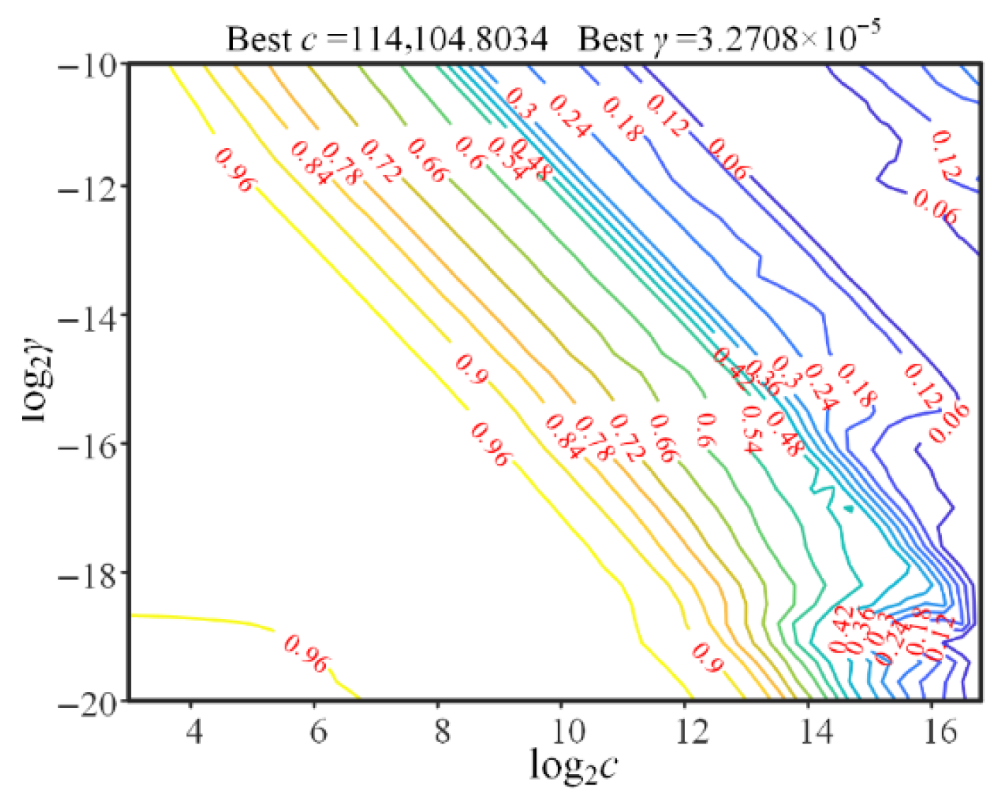
Based on the above partitioning results of the training and test samples, parameter optimization was performed on the model to obtain a relatively optimal hyperparameter combination. Taking Sample Set 3 as an example, the parameter optimization results for the SVR are shown in Figure 7. The optimal hyperparameter combination for the SVR model was determined as c* = 114104.8034 and γ = 3.271 × 10⁻⁵.

Figure 7. Results of parameter optimization for the SVR model.

The hyperparameter combinations and error metrics for the four sample sets are shown in Table 6. The results indicate that both the randomly partitioned and the non-uniformity coefficient-based sample sets achieve high prediction accuracy. Among them, Sample Set 3 was identified as the most effective, with RMSE, MAPE, and MSPE values of 0.3302, 0.0239, and 0.0132, respectively. These error metrics generally meet the requirements for practical applications.

Table 6. Optimization Parameters and Error Indicators of the Prediction Model.

Sample Set Number	1	2	3	4
C	75,281.1	114,104.8	114,104.8	2702.4
Γ	3.271 × 10−5	2.158 × 10−5	3.271 × 10−5	4.883 × 10−4
RMSE	1.5272	1.6055	0.3302	0.2515
MAPE	0.1065	0.0853	0.0239	0.0340
MSPE	0.0586	0.0533	0.0132	0.0209

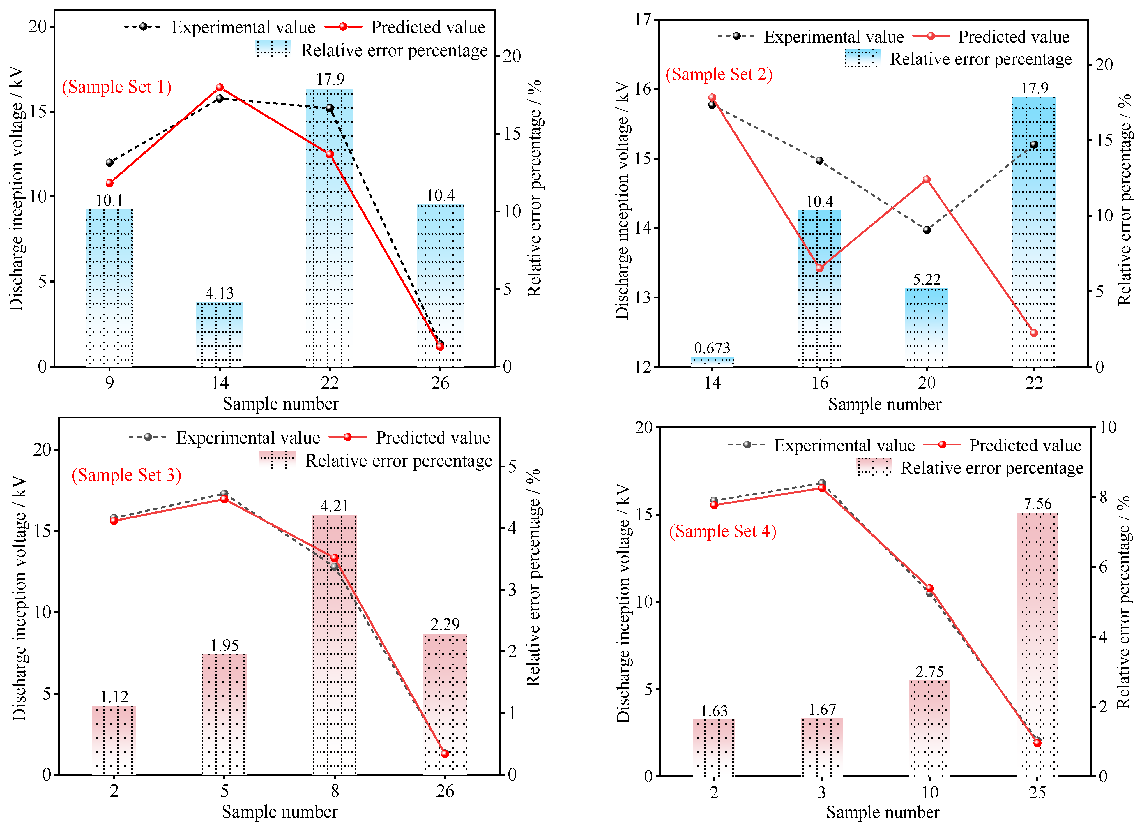
A comparison between the experimental and predicted values of the arc inception voltage for the four sample sets is shown in Figure 8. It can be observed that the sample sets partitioned based on the non-uniformity coefficient method exhibit higher prediction accuracy compared to those divided randomly. The agreement between experimental and predicted values was significantly improved, demonstrating the capability to achieve accurate predictions with a limited original sample set. Specifically, the average MAPE of Sample Sets 3 and 4 was reduced by 0.0667 compared to that of Sample Sets 1 and 2. Among all sets, Sample Set 3 achieved the lowest MAPE of only 0.0239. From the perspective of engineering practice and industry consensus, an error level of MAPE ≤ 8% can meet the accuracy requirements for practical engineering applications in the scenario of flashover voltage prediction.

Figure 8. Comparison of Arc Inception Voltage Prediction Results.

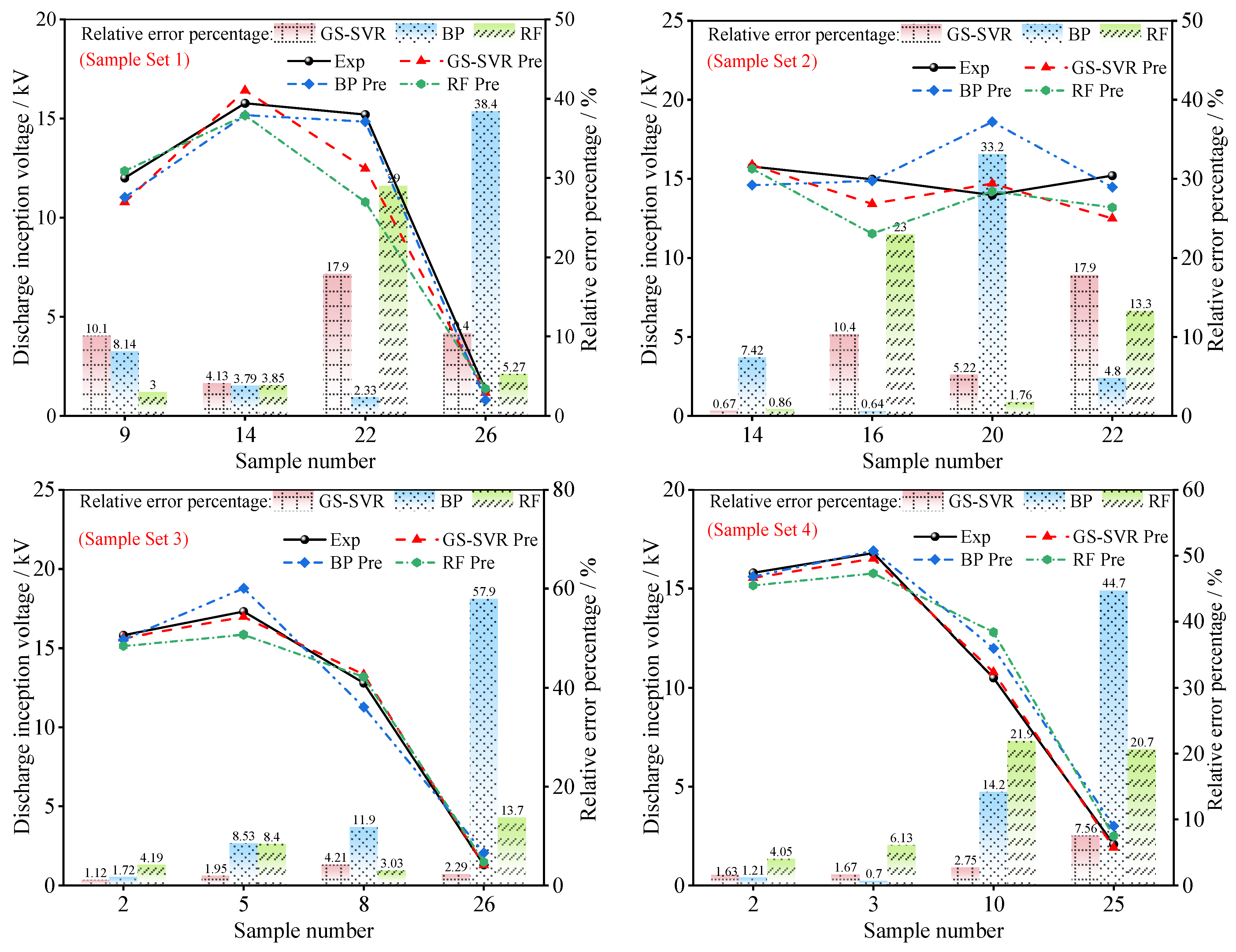
To comprehensively evaluate the predictive performance of the GS-SVR model under different sample partitioning strategies, the BP neural network and random forest (RF) were selected for comparative analysis. The BP neural network is a feedforward neural network based on the error backpropagation algorithm, achieving nonlinear mapping from input to output through multiple layers of perceptrons; random forest is an ensemble learning method consisting of multiple decision trees, and the regression prediction results are obtained by averaging the votes. The prediction results of the three models are shown in Figure 9, and the error results are presented in Table 7.

Figure 9. Comparison of the prediction results of the three algorithms.

Table 7. Comparison of errors of the three algorithms.

Set 1	GS-SVR	BP	RF	Set 2	GS-SVR	BP	RF
RMSE	1.5272	0.6492	2.2347	RMSE	1.6055	2.4166	2
MAPE	0.1065	0.1317	0.1029	MAPE	0.0853	0.115	0.0972
MSPE	0.0586	0.0988	0.0748	MSPE	0.0533	0.0858	0.0666
Set 3	GS-SVR	BP	RF	Set 4	GS-SVR	BP	RF
RMSE	0.3302	1.1315	0.8264	RMSE	0.2515	0.8855	1.3183
MAPE	0.0239	0.2	0.0734	MAPE	0.034	0.1521	0.1319
MSPE	0.0132	0.1493	0.0423	MSPE	0.0209	0.1173	0.0775

The GS-SVR prediction model maintains the lowest and evenly distributed values across all sample sets; in comparison, BP and RF show significant column heights on low-voltage or fluctuating samples and have unstable error distributions. Based on sample sets 3 and 4 optimized by the uneven coefficient division, the prediction curve of GS-SVR almost coincides with the test line, with MAPE values as low as 2.39% and 3.40%, significantly lower than those of the other two algorithms. These results fully validate the collaborative advantages of this division strategy and the GS-SVR model, achieving high-precision and high-robustness prediction of the surface arcing voltage.

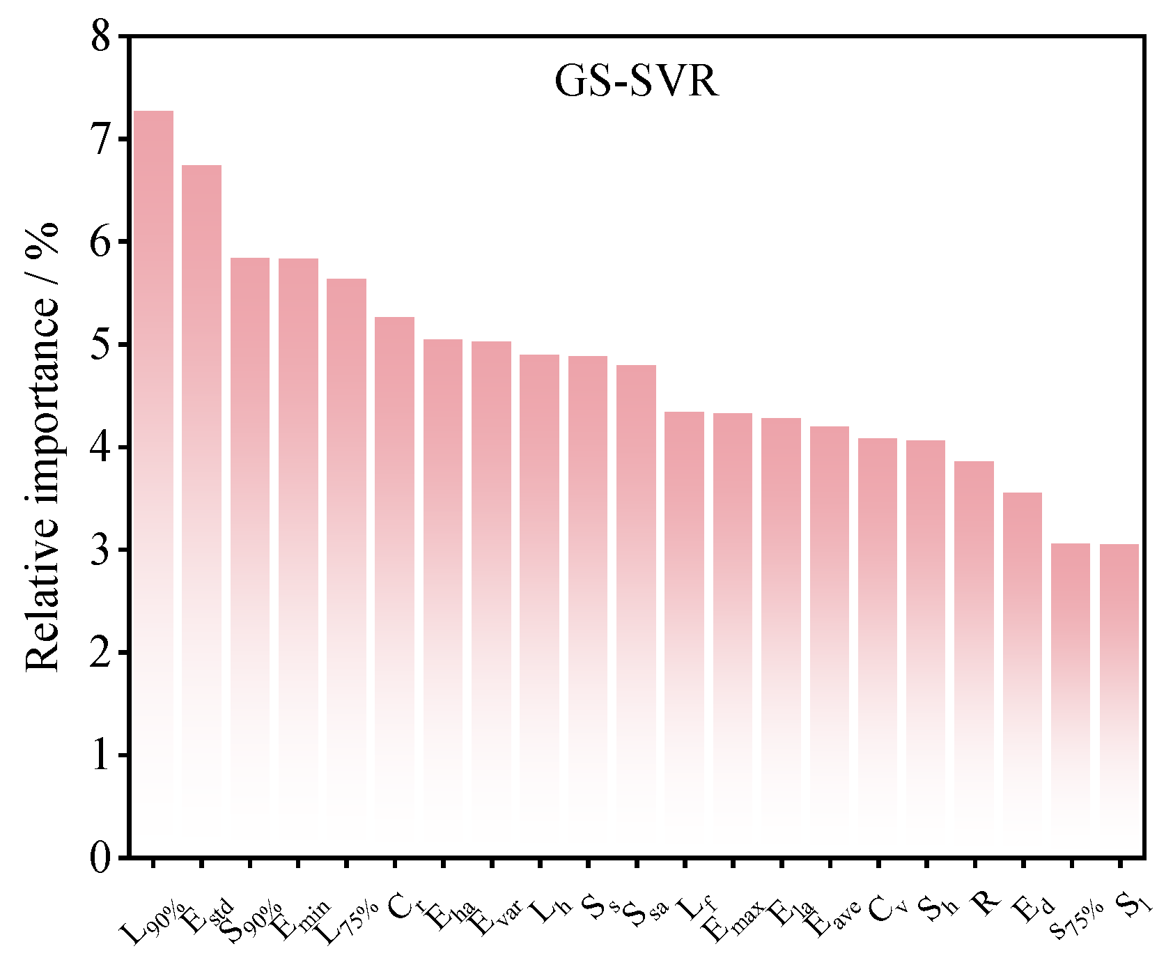
To further reveal the characteristic preference mechanism of GS-SVR in predicting the surface arcing voltage, a quantitative analysis was conducted on the relative importance of the 21-dimensional electric field feature set. The results are shown in Figure 10. The sensitivity of each feature quantity is relatively balanced, and the feature with the greatest contribution is L90%, accounting for 7.15%. The top five feature quantities, which take into account the electric field intensity, electric field energy, and local non-uniformity, have a cumulative contribution of 29.15%.

Figure 10. The contribution degree of each characteristic quantity.

4. Conclusions

In this paper, we propose a method for predicting surface arc inception voltage based on the GS-SVR algorithm, using the electric field feature set along the shortest inter-electrode path as input, achieving accurate prediction of arc inception voltage. The main contents and conclusions of this study are as follows:

(1)

A 21-dimensional electric field feature set was constructed. Using this set as input for the prediction model resulted in high agreement between predicted and experimental values. Among them, Sample Set 3 achieved the best prediction performance, with RMSE, MAPE, and MSPE values of 0.3320, 0.0239, and 0.0132, respectively.

(2)

The total sample set was partitioned using both random partitioning and non-uniformity coefficient-based partitioning methods. Compared with random partitioning, the prediction model based on non-uniformity coefficient partitioning demonstrated higher accuracy, with the average MAPE of Sample Sets 3 and 4 reduced by 6.695% compared to that of Sample Sets 1 and 2.

(3)

A surface arc inception voltage prediction model was developed using grid search optimization and support vector regression, achieving accurate prediction with a limited number of original samples. The average MAPE across all four sample sets was 6.243%. Sample Set 1 had the highest MAPE value of 10.65%; in comparison, Sample Set 3 had the lowest MAPE value of only 2.39%.

(4)

The arc inception voltage prediction model for epoxy resin under complex environmental conditions established in this study provides theoretical support for improving the insulation performance of electrical equipment under condensation conditions.

References

1. Yao, L.; Wang, Y.; Xiao, X. Concentrated Solar Power Plant Modeling for Power System Studies. IEEE Trans. Power Syst. 2024, 39, 4252–4263. [Google Scholar] [CrossRef]
2. Kumar, S.; Saket, R.K.; Dheer, D.K.; Holm-Nielsen, J.B.; Sanjeevikumar, P. Reliability enhancement of electrical power system including impacts of renewable energy sources: A comprehensive review. IET Gener. Transm. Distrib. 2020, 14, 1799–1815. [Google Scholar] [CrossRef]
3. Ji, J.; Chi, Y.; Yin, X. The blue treasure of hydrogen energy: A research of offshore wind power industry policy in China. Int. J. Hydrogen Energy 2024, 62, 99–108. [Google Scholar] [CrossRef]
4. Su, X.; Wang, X.; Xu, W.; Yuan, L.; Xiong, C.; Chen, J. Offshore Wind Power: Progress of the Edge Tool, Which Can Promote Sustainable Energy Development. Sustainability 2024, 16, 7810. [Google Scholar] [CrossRef]
5. Zhang, X.; Yang, H.; Zhou, G.; Zhao, Y.; Guo, D. Steady-state voltage stability assessment of new energy power systems with multi-quadrant power modes. Energy Rep. 2023, 9, 3851–3860. [Google Scholar] [CrossRef]
6. Shu, S.; Zhan, Z.; Xu, J.; Huang, Y.; Huang, W.; Lin, Y. Three-dimensional numerical simulation and experiment of moisture condensation mechanism inside high voltage switchgear. Electr. Power Energy Syst. 2023, 151, 109–129. [Google Scholar] [CrossRef]
7. Li, Z.; Liu, J.; Ohki, Y.; Chen, G.; Gao, H.; Li, S. Surface flashover in 50years: Theoretical models and competing mechanisms. High Volt. 2023, 8, 853–877. [Google Scholar] [CrossRef]
8. Qi, B.; Gao, C.; Li, C.; Zhao, L.; Sun, X. The influence of surface charge accumulation on flashover voltage of GIS/GIL basin insulator under various voltage stresses. Int. J. Electr. Power Energy Syst. 2019, 105, 514–520. [Google Scholar] [CrossRef]
9. Qiao, X.; Zhang, Z.; Jiang, Z.; Jiang, X.; Pang, G. Lightning Impulse Pollution Flashover Characteristics and Model of 10 kV Composite Arrester Combined Insulator. Trans. China Electrotech. Soc. 2024, 39, 6932–6940. (In Chinese) [Google Scholar]
10. Zhang, D.; Xu, H.; Huang, X.; Zhang, Z.; Jiang, X. Space Electric Field Characteristics of Silicone Rubber Insulator Pollution Flashover and Its Application in Flashover Prewarning. IEEE Trans. Dielectr. Electr. Insul. 2023, 30, 439–448. [Google Scholar] [CrossRef]
11. Wang, H.; Hu, Q.; Lin, H.; Xu, H.; Shu, L.; Yin, P.; Jiang, X. Effect of icing on the AC flashover voltage of 220 kV composite insulators. Electr. Power Syst. Res. 2025, 238, 111117. [Google Scholar] [CrossRef]
12. Wang, M.; Yuan, Y.; Jiang, X.; Li, T.; Chen, Q.; Zhou, F. Switching Impulse Flashover Performance of Nonuniform Pollution Insulators in Natural Environment. IEEE Trans. Dielectr. Electr. Insul. 2023, 30, 844–851. [Google Scholar] [CrossRef]
13. Peck, F.W. Dielectric Phenomena in High Voltage Engineering; Mc-Graw-Hill: New York, NY, USA, 1929. [Google Scholar]
14. Anderson, R.A.; Brainard, J.P. Mechanism of pulsed surface flashover involving electron-stimulated desorption. J. Appl. Phys. 1980, 51, 1414–1421. [Google Scholar] [CrossRef]
15. Sun, G.; Guo, B.; Li, W.; Zhang, S.; Zhou, R.; Song, B.; Mu, H.; Zhang, G. Estimation of surface flashover threshold in a vacuum II: Flashover phase transition. J. Phys. D Appl. Phys. 2020, 53, 075201. [Google Scholar] [CrossRef]
16. Li, Z.; Li, S.; Xu, H.; Qu, G.; Niu, H.; Huang, Y.; Aslam, F. The mechanism of gas pressure and temperature dependent surface flashover in compressed gas involving gas adsorption. Appl. Surf. Sci. 2021, 539, 148107. [Google Scholar] [CrossRef]
17. Niu, H.; Qu, G.; Li, M.; Li, Z.; Feng, Y.; Li, S. Improved surface flashover voltage of epoxy following polythiourea-assisted coating with high gas adsorption ability. Appl. Surf. Sci. 2023, 618, 156546. [Google Scholar] [CrossRef]
18. Qiu, Z.; Ruan, J.; Lu, W.; Wang, X.; Jin, Q. Feature extraction of electric field distribution and its application in discharge voltage prediction of large sphere-plane air gaps. IEEE Trans. Dielectr. Electr. Insul. 2018, 25, 1030–1038. [Google Scholar] [CrossRef]
19. Mokhnache, L.; Boubakeur, A. Prediction of the breakdown voltage in a point-barrier-plane air gap using neural networks. In Proceedings of the 2001 Annual Report Conference on Electrical Insulation and Dielectric Phenomena, Kitchener, ON, Canada, 14–17 October 2001; pp. 369–372. [Google Scholar]
20. Akram, S.; Wang, P.; Zhu, X.; Huang, J.; Liu, F.; Fang, Z. Prediction of Partial Discharge Inception Voltage for Electric Vehicle Motor Insulation Using Deep Learning. IEEE Trans. Instrum. Meas. 2023, 72, 1–10. [Google Scholar] [CrossRef]
21. Qiu, Z.; Ruan, J.; Jin, Q.; Wang, X.; Huang, D.; Shu, S. Switching impulse discharge voltage prediction of EHV and UHV transmission lines–tower air gaps by a support vector classifier. IET Gener. Transm. Distrib. 2018, 12, 3711–3717. [Google Scholar] [CrossRef]
22. Dai, H.; Mo, S.; Wang, H.; Yin, N.; Fan, S.; Li, B. Pre-insertion resistors temperature prediction based on improved WOA-SVR. IET Sci. Meas. Technol. 2024, 18, 182–192. [Google Scholar] [CrossRef]
23. Kim, J.; Kim, Y. Prediction of Positive Lightning Impulse Breakdown Voltage Under Sphere-to-Barrier-to-Plane Air Gaps Using Machine Learning. IEEE Access 2024, 12, 120429–120439. [Google Scholar] [CrossRef]
24. Qiu, Z.; Wang, X.; Ruan, J. Application of a SVR model to predict lightning impulse flashover voltages of parallel gaps for insulator strings. IEEJ Trans. Electr. Electron. Eng. 2019, 14, 1455–1462. [Google Scholar] [CrossRef]
25. Ding, C.; Zhou, Y.; Ding, Q.; Wang, Z. Loss Prediction of Ultrahigh Voltage Transmission Lines Based on EEMD–LSTM–SVR Algorithm. Front. Energy Res. 2022, 10, 811745. [Google Scholar] [CrossRef]
26. GB/T 4585-2024; Artificial Pollution Tests on High-Voltage Ceramic and Glass Insulators to be Used on a.c. Systems. China Standards Press: Beijing, China, 2024.
Disclaimer/Publisher’s Note: The statements, opinions and data contained in all publications are solely those of the individual author(s) and contributor(s) and not of MDPI and/or the editor(s). MDPI and/or the editor(s) disclaim responsibility for any injury to people or property resulting from any ideas, methods, instructions or products referred to in the content.
Article Metrics
Citations
Article Access Statistics
Multiple requests from the same IP address are counted as one view.