Abstract
Energy consumption forecasting offers a foundation for governmental agencies to establish energy consumption benchmarks for public institutions. Meanwhile, correlation analysis of institutional energy use provides clear guidance for building energy-efficient retrofits. This study employed five machine learning models to train and predict monthly energy consumption intensity data from 2020 to 2022 for three types of public institutions in China’s eastern coastal regions. A novel ensemble model was proposed and applied for energy consumption prediction. Additionally, the SHAP model was utilized to analyze the correlation between influencing factors and energy consumption data. Finally, the relationship between climatic factors and monthly energy consumption intensity was investigated. Results indicate that the ensemble model achieves higher predictive accuracy compared to other models, with regression metrics on the training set generally exceeding 0.9. Although XGBoost also demonstrated strong performance, it was less stable than the ensemble model. Energy intensity across different building types exhibited strong correlations with the number of energy users, floor area, electricity use, and water consumption. Linear analysis of temperature and energy consumption intensity revealed a directional linear relationship between the two for both medical and administrative buildings.
1. Introduction
Energy serves as a fundamental requirement for human survival [1], with carbon dioxide emitted through energy consumption being the primary source of carbon emissions. In China, energy-related CO2 emissions accounted for over 80% of the country’s total carbon emissions in 2023 [2]. The “dual carbon” vision put forward by relevant authorities has set clear targets and timelines for China’s low-carbon transition, while also presenting substantial challenges for policymakers [3]. The building sector is one of the three major energy-consuming industries globally, representing 46%, 40%, and 39% of total energy consumption in China, the United States, and Europe, respectively [4,5]. Notably, the operational phase of public buildings contributes significantly to carbon emissions, accounting for 38% of total building operational carbon emissions in 2020, thus representing a critical domain for energy conservation and emission reduction efforts [6].
Accurately assessing building energy consumption and disentangling the effects of various influencing factors are essential tasks [7]. Researchers often develop predictive models to estimate building energy use. Among these, physics-based models rely on thermal principles and require inputs such as building characteristics and environmental parameters to solve thermal balance equations [8,9]. In contrast, data-driven models only need historical energy consumption data to train the algorithm. As a result, data-driven approaches have gained increasing popularity in recent years for predicting and evaluating energy performance in the building sector.
In terms of the annual total energy consumption of regional buildings, Gyanesh et al. [10] and Rafael et al. [11] compared the predictive performance of multiple models for over 2000 residential buildings in India and over 700 office buildings in Chile, respectively. The results indicated that the hybrid model was more suitable for energy consumption predictions of residential buildings. ANN and linear models were more suitable for energy consumption predictions in office buildings. In terms of annual unit area energy consumption (EUI) predictions, Yalcintas et al. [12] found that the ANN model performed better in predicting the EUI of buildings in the CBECS library compared to other models. Roth et al. [13] found that both RF and Gaussian regression models performed well in predictions. Matheus et al. [14] and Zhang et al. [15] both predicted the EUI of educational buildings. The results showed that the Bayesian discretization method had higher prediction accuracy for discrete samples. In addition, the prediction results of CNN-LSTM-Attention were more accurate compared to other neural networks, but required more training time than other models. Cui et al. [16] predicted EUI for 1169 apartments and 4231 single family homes based on three ensemble tree models in the RECS library. It was found that the LightGBM was most suitable for predicting energy consumption in apartments, while the CatBoost was most suitable for predicting energy consumption in single household residences.
Some researchers have also conducted predictive studies on sub item energy consumption in buildings. Robinson et al. [17] predicted the annual main fuel consumption of 13,223 buildings in New York City in the CBECS database based on multiple machine learning models. The gradient boosting model was found to have more accurate prediction results. Abdo et al. [18] predicted the annual electricity and natural gas consumption of nearly 10,000 households in London according to multi-layer neural networks, linear regression, RF, and gradient boosting models. The results indicated that multi-layer neural networks had the best prediction performance, followed by the RF. Li et al. [19] predicted the power consumption of Türkiye’s transmission companies for about 400 months based on XGBoost, CatBoost, and three model optimization methods. The XGBoost model was found to have excellent performance in predicting electricity consumption.
The preceding review reveals a diverse application of models in building energy prediction. However, a comparative analysis across these studies yields critical insights into the relative strengths of each algorithm, which are highly dependent on dataset size, feature complexity, and the nature of the prediction task. ANNs typically excel with very large datasets (e.g., >10,000 samples) where their deep architecture can learn complex, nonlinear representations without overfitting. However, on smaller datasets, such as those common in institutional-level studies, ANNs are highly prone to overfitting, leading to poor generalization, despite their theoretical capacity. RF are robust and less prone to overfitting than ANNs due to their ensemble “bagging” nature. They perform reliably across various dataset sizes and provide good feature importance estimates. However, RF can sometimes be outperformed by boosting algorithms in terms of pure predictive accuracy, as it may not fully optimize for the hardest-to-predict samples. Gradient boosting machines consistently demonstrate superior performance on small- to medium-sized, heterogeneous datasets—precisely the profile of our study. The sequential, error-correcting nature of boosting allows GBMs to build a strong predictor by focusing on residual errors from previous models. This makes them exceptionally adept at capturing complex, nonlinear relationships and interaction effects among multiple features without requiring an excessively large sample size. It is very suitable for samples with multiple characteristics but small scale in building energy consumption.
What are the key driving factors influencing energy consumption in each type of institution? Overall, most current research focuses on the annual energy consumption of buildings. However, existing studies on public institution energy consumption predominantly rely on annual or quarterly data. This coarse temporal resolution obscures the dynamic patterns of energy use at the monthly level. Crucially, the impact of climate variables on energy demand—such as summer cooling and winter heating—is most pronounced at this monthly scale. Annual data fails to capture these short-term fluctuations and the immediate impact of extreme weather events. Consequently, a critical research gap exists in the systematic modeling of monthly energy intensity and its drivers across different types of public institutions (EI, AI, MI). This gap currently hinders the development of precision energy-saving policies that are synchronized with operational cycles. Clarifying the climate–energy intensity relationship at a monthly resolution has direct implications for operational policy decisions within public institutions. For instance, the differential response patterns to high and low temperatures across institution types, which this study aims to uncover, can provide a quantitative basis for specific actions. It could provide budgeting, procurement, maintenance scheduling, flexible work arrangements, and space management.
Therefore, the study evaluated the predictive performance of monthly operating energy consumption of regional public institutions based on multiple machine learning models. The research predicts that the ensemble model will achieve significantly lower prediction errors (e.g., lower RMSE) compared to individual models across all institution types. Subsequently, the SHAP model and linear regression were employed to explore the impact of temperature and various influencing factors on energy consumption. The research provides guidance and suggestions for the formulation of energy-saving policies in future construction related departments.
2. Methods
Figure 1 is the flowchart of the research. It outlined a structured methodology for energy consumption prediction, integrating data-driven modeling and climate impact analysis. The process began with data acquisition and preprocessing to ensure input data quality. Subsequently, multiple optimized prediction models—including SSA-RF, SSA-SVM, SSA-XGBoost, and SSA-BP—were constructed and compared through model selection and performance comparison. An SSA-Ensemble model might also be developed to enhance robustness. The optimal model was then interpreted using the SHAP model for feature importance analysis, facilitating the exploration of climate impact. The final output is an accurate and interpretable energy consumption prediction, providing valuable insights for energy planning and policy-making.
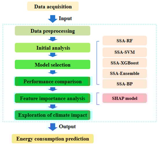
Figure 1.
Flowchart of the research.
2.1. Data Sources
Based on the Chinese national standard GB/T 40498-2021 (general principles of drafting energy consumption norm standards for public institutions) [20], a structured questionnaire was designed to collect energy consumption data from approximately 250 public institutions in eastern coastal China through quarterly surveys from 2020 to 2022. It covered three categories—educational (EI), administrative (AI), and medical institutions (MI). The questionnaire encompassed six sections: basic building information, energy consumption data, major energy-consuming equipment, renewable energy statistics, energy-saving renovations, and energy metering details, with the energy consumption section being the most critical as it required monthly reporting of electricity, water, natural gas, and IT server room usage. Through systematic collection and organization of the data, two dependent variables—monthly per capita energy consumption (PCEC) and monthly energy consumption per unit building area (ECPUA)—were defined for analysis, while the specific independent variables, along with their abbreviations and units, are summarized in Table 1.

Table 1.
Interpretation and units of different features.
Usually, according to JGSW01-2021 (energy and resource consumption quota of central and state organs), the calculation method for monthly total institution energy consumption was the sum of the actual physical consumption of various energy sources in the current month [21]. The impact of local temperature and air quality on energy consumption could not be ignored, as they could affect the operation of air conditioning and thus alter institution energy consumption. This study also inputted the month and year of building energy consumption as unique heat codes into the model. The comparison of all abbreviations in the study is shown in Table 1 and the Abbreviations part.
2.2. Data Preprocessing
For the energy and resource consumption data of public institutions, the types of missing data include the following:
- (1)
- Missing key energy consumption data: Instances where data such as comprehensive energy consumption, building energy consumption, or electricity consumption were missing. Such samples were directly discarded.
- (2)
- Missing key institutional information: Instances where data such as building area were missing. These were imputed using the median value from the corresponding historical reporting series of the public institution to which the sample belongs. The median value is not sensitive to outliers, while energy consumption data often contains outliers caused by special events such as extreme weather, equipment failures, or temporary activities. Historical energy consumption data often presents a skewed distribution (for example, a right-skewed distribution, where a few institutions have extremely high consumption). In a skewed distribution, the median is better able to reflect the central trend than the mean, avoiding estimates being pulled up or down by a few extreme values. If imputation was not possible, the sample was directly discarded.
Additionally, the logical consistency of attribute relationships within the dataset must be validated. For example, total fuel consumption should equal the sum of vehicle fuel consumption and other fuel consumption. Samples violating these data relationship rules were directly discarded.
To screen for anomalous data points, zero values in energy and power consumption records were first removed. The remaining dataset was then processed using the interquartile range (IQR) method, where IQR is defined as the difference between the upper quartile (UQ) and the lower quartile (LQ). Observations falling outside 1.5 times the IQR were classified as mild outliers, a widely accepted statistical threshold that offers a balanced approach to identifying extreme values without oversimplifying the underlying data structure. This method is particularly suitable for building energy data, which often exhibits right-skewed distributions. Prior to outlier detection, quantile transformation was applied to approximate a normal distribution of energy consumption values. The 3IQR test was subsequently conducted on the training set, and values identified as outliers—deemed unlikely to represent true operational conditions—were excluded. As summarized in Table 2, the removed outliers accounted for less than 5% of the total dataset. These anomalies may have resulted from damaged meter bases, erroneous reporting, or equipment malfunction. Variations in sample sizes across institution categories reflect their real-world distribution and data accessibility in the study region, with educational institutions being more numerous and having more systematic energy reporting practices compared to medical institutions, which are fewer in number and often maintain less accessible energy records.
Table 2.
The available data volume and excluded data volume of various types of institutions.
2.3. Model Selection
This study adopted a methodological strategy involving five distinct prediction models to effectively identify the most suitable approach for different institution types and monthly energy consumption patterns. Given their recognized strong adaptability and rapid training speed, two of the most widely used ensemble models were included in this selection. The back propagation neural network model (BP) has advantages in prediction accuracy for large datasets. And the support vector machine (SVM) model is also commonly used for energy consumption predictions. In addition, the ensemble model was specifically constructed for monthly energy intensity prediction in the study. The training of all models used was completed in Python (3.12). Among them, RF, SVM, GBDT, and BP were from scikit-learn (0.24.2). XGBoost was from the standard XGBRegressor. All calculations were based on a GPU running on RTX3060.
2.3.1. Random Forests
RF is a type of tree model, whose core principle is to integrate multiple weak decision tree models into a strong model [22]. Unlike gradient boosting models such as GBR, RF adopt a nested ensemble architecture. Finally, by weighted averaging of the training results of all decision trees, the regression prediction results can be obtained. RF has strong robustness to outliers and noise, is less prone to overfitting when the noise is low, and has a faster training speed than gradient boosting models.
2.3.2. Support Vector Regression
The core idea of SVM models is to map the original training set to a high-dimensional feature space, and balance accuracy and computational complexity through loss functions and penalty factors [23]. The principle is to find a discriminative linear binary classifier with the maximum separation hyperplane in the feature space, thereby achieving the highest robustness of the model. Essentially, it can be seen as solving high-dimensional quadratic regression problems. The SVR algorithm is mainly divided into three types: soft-interval SVR, hard-interval SVR, and kernel SVR. Normally, interval SVR is used to handle linear correlation problems, while kernel SVR is used to handle nonlinear correlation problems.
2.3.3. XGBoost
eXtreme gradient boosting (XGBoost) is an improved version developed based on the gradient boosting algorithm [24]. Its core innovation lies in using the second-order derivative of Taylor expansion for calculation during the gradient boosting process, while traditional GBR is only based on the first-order derivative. The use of this second-order derivative makes the gradient boosting algorithm superior in terms of prediction speed and accuracy [25]. In addition, XGBoost introduces regularization terms during the decision tree construction phase to prevent model overfitting. Although the training speed is faster, each learning stage requires processing a complete dataset and occupies more storage space.
2.3.4. Back Propagation Neural Network
BP is a multi-layer feedforward network trained by error back propagation [26]. Its basic idea is gradient descent, which is based on using gradient search techniques to minimize the mean square error between the actual output value and the expected output value of the network. The basic BP includes two processes: forward propagation of signals and backward propagation of errors. When calculating the error output, it is performed in the direction from input to output, while adjusting the weights and thresholds is performed in the direction from output to input. BP can approximate any nonlinear continuous function, which enables it to handle complex internal mechanism problems. In addition, even if some neurons are damaged, the BP can still function normally, demonstrating a certain level of robustness [27]. However, due to its gradient descent approach, the network may converge to local minima rather than global optima. Neural networks also have a high desire for data volume.
2.3.5. Ensemble Model
In order to find a better model for predicting the energy consumption intensity of public institutions, the study proposed an ensemble model. The principle was shown in Figure 2. XGBoost is an optimization algorithm for GBDT. GBDT is based on first-order derivatives, which is relatively simple but stable [28]. Therefore, for specific datasets, GBDT may have better regression performance. The XGBoost and GBDT, trained separately, were weighted and combined. The optimal values of weights ω1 and ω2 were searched for based on a sparrow search algorithm (SSA). The goal of the optimization algorithm was to minimize mean squared error (MSE).
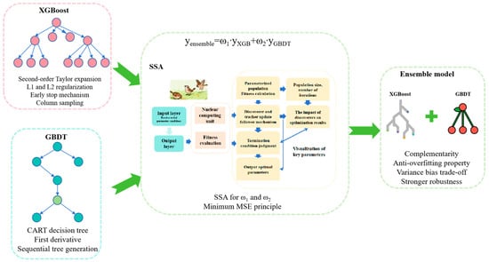
Figure 2.
Schematic diagram of ensemble model.
The ensemble model had the advantage of two complementary algorithms. XGBoost had the strong ability to capture complex nonlinear relationships, while GBDT was more robust to noisy data. The difference between the two algorithms provided model diversity and reduced the deviation of a single model. A single model might have variance or bias. Ensemble models could achieve better variance–bias trade-offs. Therefore, by optimizing the weights, the model found the optimal balance point. XGBoost and GBDT might capture different feature interaction patterns, so the ensemble model could comprehensively utilize different interaction information. The combination model was automatically searched for the best weight combination based on SSA, avoiding the subjectivity of manually setting weights.
2.4. Sparrow Search Algorithm
Due to the significant impact of hyperparameters on the algorithm, the study adopted SSA to automatically optimize the parameters. This optimization strategy draws inspiration from the foraging principles of sparrow populations [29]. The sparrow population is divided into three categories: discoverers, followers, and sentinels. They search efficiently for the optimal solution in the solution space by simulating their interactions and position update strategies. The discoverer is responsible for searching for areas rich in food. Followers follow the discoverer to areas with abundant food and conduct a detailed local search around the discoverer. They are vigilant, always alert to dangers in the environment (such as predators). When danger approaches, they will sound an alarm and drive the entire population to abandon the current food source and randomly move to a new safe location to avoid the population falling into a local optimum [30]. In each iteration, roles will be reassigned according to individual fitness values. The ones with the best adaptability become discoverers, those with poor adaptability become sentinels, and the rest become followers. SSA has strong global exploration capabilities and efficient local development capabilities. In addition, its good ability to jump out of local optima and fast convergence speed are also its characteristics. The parameters of SSA in this study were set as follows:
pop_size = 20, n_iter = 30, lb = [50, 3, 0.01, 0.6, 0.6, 0.1, 0.1], ub = [200, 8, 0.1, 0.9, 0.9, 1.0, 1.0], dim = 7/2.
2.5. Performance Standards
In order to find the best model for predicting carbon emissions of different types of institutions, the following four indicators were selected to compare the predictive performance of different models [4,31,32]. In addition, all models were subjected to 5-fold cross validation and the performance parameters were averaged. Using 5-fold CV allowed us to perform a more extensive hyperparameter tuning and model evaluation within a feasible time frame, given our available computational resources.
The coefficient of determination (R2) is a commonly employed metric in regression analysis, representing the proportion of variance in the dependent variable that is predictable from the independent variables. Its definition formula is as follows:
where n is the number of samples, and are the true and predicted values of the ith sample, and is the average value of the samples.
The root mean square error (RMSE) is a standard metric for evaluating the accuracy of continuous predictive models. It represents the standard deviation of the residuals (prediction errors), quantifying the average magnitude of deviation between predicted and actual values. RMSE is defined as follows:
Mean absolute error (MAE) represents the average error between the predicted value and the true value. It is defined as follows:
The mean bias error (MBE) measures the average bias in predictions, indicating the model’s tendency to overestimate (positive MBE) or underestimate (negative MBE). A lower absolute MBE value signifies better predictive accuracy. It is defined as follows:
Normalized root mean square error (NRMSE) is a normalized version of root mean square error. It eliminates the influence of absolute size and dimensionality of data by dividing RMSE by a representative value of the observed values (such as the range or mean), thus making the errors of different datasets or models comparable. It is defined as follows:
Normalized mean bias error (NMBE) is used to measure the systematic bias (overestimation or underestimation) of model predictions. It calculates the average deviation between predicted and observed values and normalizes them, usually using the average or range of observed values to eliminate dimensional effects. It mainly reflects the average offset direction and degree of the system, rather than the accuracy of prediction. It is defined as follows:
2.6. SHAP Value Algorithm
The SHapley Additive exPlanations (SHAP) algorithm belongs to the post model interpretation method. Its core idea is to analyze the “black box model” from both global and local levels by calculating the marginal contribution of features to the model output. This method is based on cooperative game theory to assign significant values to each feature based on the predicted results, with local accuracy, missing rate, and consistency as three parameters. Compared to the feature importance provided by tree models, SHAP can provide the local feature importance of a single sample, and the feature contribution values have directionality. Meanwhile, the global feature importance is calculated based on the feature importance set of the sample set. The SHAP method is also an additive feature attribution method, which changes the results by adding or removing specific features to each feature subset. In addition, SHAP can be applied to various interpretation scenarios such as deep learning models, tree models, gradient machines, etc.
3. Results and Discussion
3.1. Sample Data Analysis
Figure 3 shows the statistical box plot of monthly PCEC and ECPUA of three types of public buildings in the eastern coastal areas of China from 2020 to 2022. Overall, there was a phenomenon in the three types of building energy consumption samples where a small portion of high energy consumption data appeared outside the upper quartile inner column. The median lines were all located below the mean. This indicated that the data with lower energy consumption in the samples had a higher density. However, it was observed that the data outside these inner columns had stronger continuity, so they could not be considered as outlier processing.
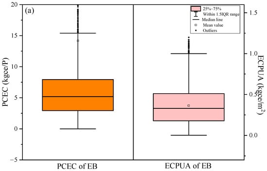
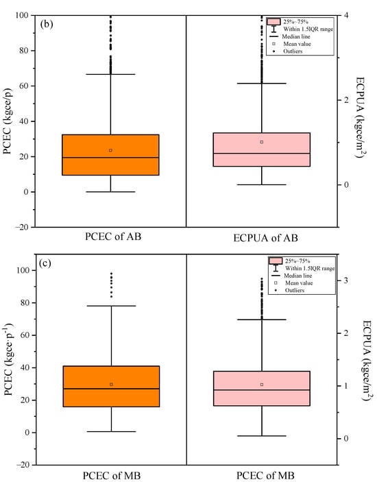
Figure 3.
Per capita energy consumption (PCEC: orange) and energy consumption per unit area (ECPUA: pink) of various types of buildings: (a) Educational buildings (EB); (b) Administrative buildings (AB); (c) Medical buildings (MB). IQR is interquartile range.
For PCEC, EI had the lowest energy consumption among the three types of buildings, ranging from 0 to 20 kgce/P. This was often related to the low-energy consumption behavior of personnel in EI and two long holidays every year. The monthly PCEC of MI was the highest, ranging from 0 to 100 kgce/P, with an average of 29.8 kgce/P. It was consistent with our previous research [33]. This was because for common public institutions, MI needed to meet the daily operating conditions of medical equipment and air conditioning equipment, and there was minimal rest throughout the year. So the energy consumption value was relatively high. The PCEC of AI was lower than that of MI. For ECPUA, the comparison results of the energy consumption values of the three types of public institutions were similar to PCEC. The ECPUA of EI was the smallest, between 0 and 1.25 kgce/m2. It could be seen that the difference between the average and median ECPUA of EI was smaller compared to the difference in PCEC, because the overall numerical magnitude of the unit building area was smaller and more concentrated.
Figure 4 shows the monthly variation curves of PCEC and ECPUA for three types of public institutions over a period of three years. Overall, the monthly changes in PCEC and ECPUA between AI and MI were more pronounced. The peak periods of energy intensity were from June to September and from January to March each year. This is because these two time periods were the hot and cold seasons in the local area, and institutions needed to overcome seasonal conditions to increase energy demand. And other months were suitable for climate, so energy demand decreased. For EI, PCEC exhibited a similar pattern to other institutions, while ECPUA did not show a more obvious pattern. This is related to the unique winter and summer vacation system of EI. During the winter and summer vacations, students and faculty members might experience reduced energy consumption due to holidays, leading to unpredictable changes in ECPUA. Therefore, from the perspective of regularity integrity, PCEC had more data stability compared to ECPUA.
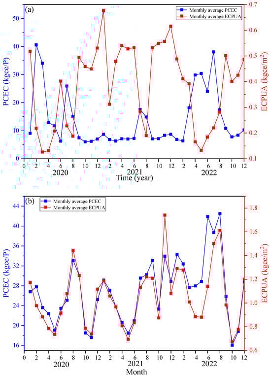
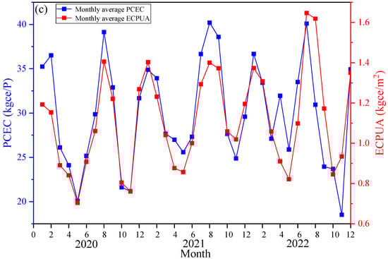
Figure 4.
Monthly change curve of PCEC and ECPUA in public institutions: (a) Educational institutions; (b) Administrative institutions; (c) Medical institutions.
Figure 5 shows the Pearson correlation analysis results of PCEC, ECPUA, and 13 related influencing factors for three institutions. Overall, there was a strong linear correlation between the temperature related influencing factors. There was a strong negative linear correlation between AQ and the temperature related influencing factors. For EI and AI, there was a correlation between NGV and NNV. But for EI and MI, there was a significant correlation among BA, NEU, and H. This was because the scale of both types of institutions was directly proportional to these factors.
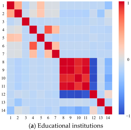
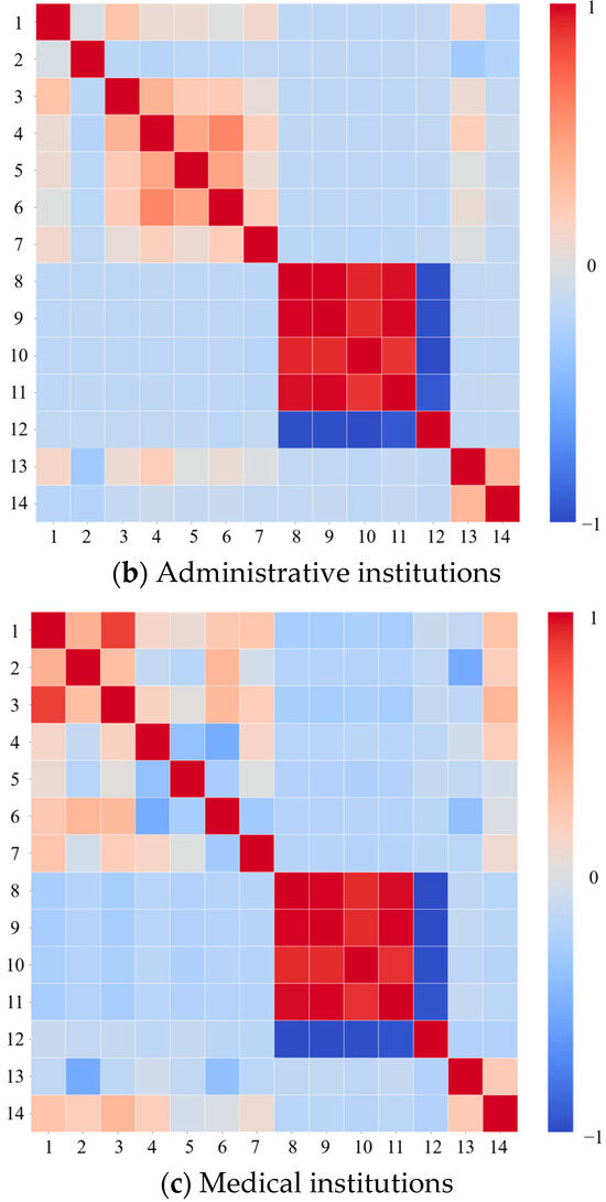
Figure 5.
Pearson correlation analysis results of influencing factors of public institutions. Features 1 to 14, respectively, represent building area, number of energy users, headcount, number of gasoline vehicles, number of diesel vehicles, number of new energy vehicles, number of charging stations, average high temperature, average low temperature, extremely high temperature, extremely low temperature, air quality, energy consumption per unit building area, and per capita energy consumption. Among them, features 1 to 13 are consistent with Table 1.
3.2. Comparison of Prediction Results of Different Models
In order to enhance the generalization of the model, the study used samples from 2020 and 2021 as the training set and samples from 2022 as the testing set. During the model training process, a 5-fold cross validation method was used. In addition, based on the VIF results of the features and to avoid the risk of data leakage, EC, WC, and NV were excluded from the features in the study. Due to the right-handed distribution of energy consumption data, in order not to affect prediction performance, logarithmic transformation was performed on the energy consumption data before training. And the data was inverse transformed after training and prediction. The predictive performance parameters were calculated based on actual data. Table 3 and Table 4 show the predictive performance of different models for monthly PCEC of three institutions. According to Table 3, the regression index R2 of XGBoost and the ensemble model were the highest. Their R2 values were basically the same. They were all above 0.95 and their MAE, MBE, NMBE, RMSE, and NRMSE were all the smallest, indicating that their fitting abilities were the strongest. The next level was RF. SVM and BP showed underfitting. This was because the sample size was not large enough and there were many feature vectors.
Table 3.
Performance results of different models for predicting monthly per capita energy consumption of training set.
Table 4.
Performance results of different models for predicting monthly energy consumption per unit area of training set.
According to Table 4, the regression index R2 of XGBoost and the ensemble model were still the highest. They were all above 0.9. In addition, the R2 of the ensemble model was slightly higher than XGBoost. The other three parameters were also lower. This indicated that the stability and generalization of the ensemble model were stronger than for XGBoost, consistent with the previous statement. The performance of the other three model test sets was average. This indicated that gradient boosting models were more suitable for regression prediction of small-scale and multi-feature samples. Furthermore, it could be seen that the small sample size of medical institutions had almost no impact on the model regression.
Table 5 and Table 6 show the predictive performance of different models for monthly ECPUA of three institutions. Overall, the prediction accuracy of ECPUA was slightly worse than PCEC, which might be due to the fact that the features in the sample were more consistent with prediction for PCEC. According to Table 5, RF, XGBoost, and ensemble models all have good training performance with the training set. This was similar to the prediction results of PCEC. Table 6 showed that the prediction accuracy of all models had decreased on the test set. However, the R2 of XGBoost and the ensemble model still remained above 0.9. Prediction performance of AB was better than the other two institutions. This was because there was more noise in the samples of the other two institutions. The ensemble model had better predictive performance than XGBoost. The research of Robinson also found that XGBoost had a higher regression index compared to other models [17]. However, the R2 of XGBoost in the research was generally lower than 0.9, while our ensemble model performed better. However, this was also related to the quality of the sample. In the research of Gassar, the XGB model exhibited unstable performance [18]. This was because XGBoost was easily troubled by local optimal solutions. This problem had been well addressed in our research using the ensemble model. For the convenience of observing the performance improvement of the combined model, the rate of change and p-value of the ensemble model parameters for the combined model are shown in Table 7. For the convenience of observing the performance improvement of the combined model, the rate of change and p-value of the ensemble model parameters for the combined model are shown in Table 7. It could be seen that the performance parameters of the ensemble model meet the correlation test with the parameters of the benchmark model. And all performance parameters had been improved to some extent.
Table 5.
Performance results of different models for predicting monthly per capita energy consumption of test set.
Table 6.
Performance results of different models for predicting monthly energy consumption per unit area of test set.
Table 7.
The rate of change and p-value of baseline model parameters for the ensemble model.
Figure 6, Figure 7 and Figure 8 present a comprehensive comparison between the predicted values and actual measurements of monthly per capita energy consumption and monthly energy consumption per unit area across three distinct institutional types using the optimized ensemble model. The scatter plots demonstrated a strong alignment between predicted and actual values, with data points clustering closely along the diagonal reference line, indicating the model’s robust predictive accuracy. This close correspondence was particularly evident in the educational institution data (Figure 6), where the ensemble model successfully captured the complex energy consumption patterns across different operational scales.
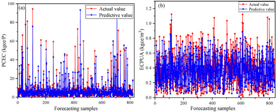
Figure 6.
Comparison between predicted values and reality of educational institution: (a) Monthly per capita energy consumption; (b) Monthly energy consumption per unit area.
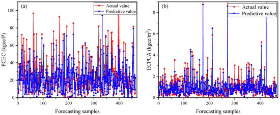
Figure 7.
Comparison between predicted values and reality of administrative institution: (a) Monthly per capita energy consumption; (b) Monthly energy consumption per unit area.
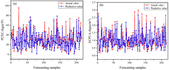
Figure 8.
Comparison between predicted values and reality of medical institution: (a) Monthly per capita energy consumption; (b) Monthly energy consumption per unit area.
Notably, the model exhibited excellent generalization capability across diverse institutional categories, maintaining consistent predictive performance despite the inherent differences in operational characteristics, usage patterns, and energy demand profiles. The slight systematic underestimation observed across all institutional types, where predicted values tend to fall marginally below the actual measurements, warrants detailed consideration. This prediction bias could be attributed to several interconnected factors. Primarily, the inherent class imbalance in the training dataset, characterized by an overrepresentation of moderate consumption patterns and underrepresentation of extreme high-consumption instances, introduced a conservative bias in the model’s predictions. The ensemble algorithm, while effective in capturing general trends, demonstrated a tendency to regress toward the mean when confronted with outlier scenarios or rare high-consumption events.
3.3. Feature Importance Analysis Based on SHAP
Feature importance analysis is of great significance for evaluating the global interpretability of models. Figure 9 and Figure 10 demonstrate the feature importance of the global perspective based on SHAP model for predicting carbon emission intensity of various institutions (only the 14 most influential factors were shown in the figure). The energy consumption patterns of educational institutions exhibited significant personnel led characteristics. The NEU occupied an absolute dominant position in per capita energy consumption predictions, reflecting the essential characteristics of personnel density in educational activities. BA, as a key indicator of infrastructure carrying capacity, together with personnel factors constituted the dual core driving force of educational energy consumption. It is worth noting that the importance of EHT went beyond conventional climate variables, reflecting the special vulnerability of educational institutions under extreme climate conditions, and it might be closely related to summer school activities and centralized use of air conditioning systems. Administrative institutions exhibited a more balanced multi-factor driving model. NEU and BA were almost equally important, reflecting the dual dependence of administrative office energy consumption. The prominent importance of NV revealed the significant role of administrative transportation in energy consumption, which was relatively weaker in other types of institutions. In temperature variables, the importance of AHT exceeded that of extreme temperature, indicating the sensitivity of administrative agencies to conventional seasonal climate change. The energy consumption of medical institutions presented a highly personnel intensive characteristic, with the importance of NEU reaching the peak among the three types of institutions, highlighting the extreme dependence of medical services on human resources. The importance of BA was relatively balanced, while the significant impact of AHT reflected the strict temperature control requirements of medical institutions, which were directly related to the operating environment of medical equipment, drug storage conditions, and patient comfort needs.
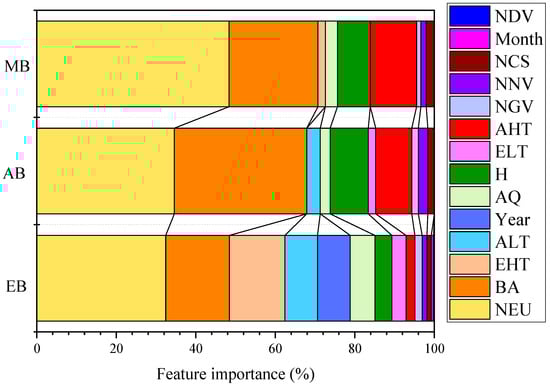
Figure 9.
The feature importance of monthly per capita energy consumption predictions of different public institutions based on the SHAP model. (EI) Educational institutions; (MI) Medical institutions; (AI) Administrative institutions.
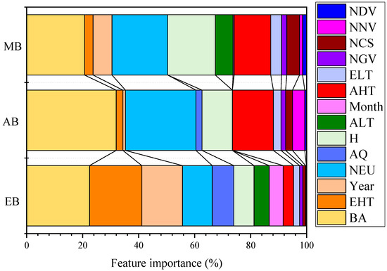
Figure 10.
The feature importance of monthly energy consumption per unit area predictions of different public institutions based on the SHAP model. (EI) Educational institutions; (MI) Medical institutions; (AI) Administrative institutions.
There were both commonalities and significant differences in the energy consumption driving mechanisms among the three types of institutions. Personnel factors occupied a central position in all types of institutions, but their impact intensity had a clear gradient: medical institutions > administrative institutions > educational institutions. The impact patterns of building factors varied, and were most prominent in the unit area energy consumption predictions of administrative institutions. The impact of climate factors exhibited institutional specificity: educational institutions were sensitive to extreme events, administrative institutions responded significantly to seasonal changes, and medical institutions demonstrated a sustained need for temperature control.
The impact of transportation factors was particularly significant in administrative agencies, reflecting the essential differences in operational models and organizational structures among different institutions. This differentiated feature importance model provided an important theoretical basis for formulating precise energy efficiency policies specific to institutions, emphasizing the necessity of differentiated energy management strategies based on institutional functional positioning and operational characteristics.
3.4. Exploration of the Relationship Between Temperature Factors and Energy Consumption Intensity
The previous section found that climate factors did indeed affect the energy consumption intensity of public institutions. To further investigate the impact of temperature on energy consumption intensity, the monthly AHT, monthly ALT, and PCEC were combined for research. Because the previous conclusion indicated that the monthly changes in PCEC were more regular than those in ECPUA, usually air conditioning was affected by external temperature in two directions. When the temperature was too high, the air conditioner heated up. When the temperature was too low, the air conditioner cooled down. Both directions were reasons for the increase in energy consumption. Therefore, this section divided AHT and ALT into two directions: a high temperature zone and a low temperature zone. AHT with a temperature above 22 °C was defined as the high temperature zone, while AHT with a temperature below 22 °C was defined as the low temperature zone. For ALT, a temperature above 15 °C was defined as the high temperature zone, while a temperature below 15 °C was defined as the low temperature zone. Temperatures of 22 °C and 15 °C were the arithmetic means.
Figure 11 and Figures S1–S3 show the relationship between temperature distribution and PCEC under four different scenarios. Overall, there was a clear positive correlation between the high temperature zone temperatures and PCEC in MI and AI. And there was a clear negative correlation between their low temperature zone temperatures and PCEC. For EI, there was no significant correlation, which was also due to their winter and summer vacations. And the air conditioning equipment and opening hours of EI were usually not as frequent as the other two types of institutions. For MI and AI, the correlation slope between temperature in the high temperature zone and PCEC was greater. This phenomenon primarily stems from fundamental differences in the physics and operational patterns of cooling versus heating systems in buildings. Firstly, the efficiency of electrically driven cooling systems degrades sharply as ambient temperature rises. When outdoor temperatures exceed 35 °C, heat rejection becomes difficult, forcing the compressor to work significantly harder to maintain the indoor setpoint, leading to a super-linear increase in electricity consumption. In contrast, the efficiency of common heating systems (e.g., gas boilers) is less affected by low outdoor temperatures, resulting in a more linear energy increase. Secondly, MI and AI institutions generate substantial internal heat from occupants, lighting, office equipment, and particularly in MIs, medical devices. During high temperatures, this internal heat adds to the external heat gain, collectively burdening the cooling system and causing a sharp energy rise. Conversely, during low temperatures, these internal sources offset a portion of the building’s heat loss, mitigating the heating load and flattening the energy-increase curve. Finally, especially for MIs, critical areas like operating rooms and laboratories require strict, year-round temperature control. The significant heat emitted by medical equipment creates a substantial base cooling load even in mild weather. During extreme heat events, this base load combines with the additional cooling demand, amplifying the sensitivity of energy consumption to high temperatures.
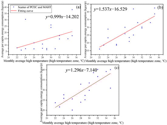
Figure 11.
The relationship diagram between PCEC of different institutions and AHT in high temperature zones. (a) Educational institutions; (b) Medical institutions; (c) Administrative institutions.
Their linear formulas are y = 1.537x + 16.529 and y = 1.296x − 7.140. The slopes all exceed 1. Furthermore, from the intercept, it can be seen that at the same temperature, the PCEC of MI was higher. This is consistent with the previous conclusion. In addition, the slope of the linear relationship between their low temperature zone temperature and PCEC is higher than −1. This indicates that the impact of extreme heat on PCEC was greater than that of extreme cold.
4. Conclusions
This study predicted the monthly energy consumption intensity of different types of public institutions in the eastern coastal areas of China based on five models. A new ensemble model was proposed and applied. And the SHAP model was used to explore the importance of energy consumption characteristics. In addition, the relationship between climate factors and energy consumption intensity was explored. The main conclusions of this study are as follows:
- (1)
- EI had the lowest monthly energy consumption among the three types of institution, while MI had the highest monthly energy consumption among the three types of institution. The regularity of monthly energy intensity changes in AI and MI is stronger than that in EI.
- (2)
- Through model performance analysis, XGBoost and ensemble models had the best predictive performance in the training set. In the test set, the energy consumption intensity prediction performance of the ensemble model was more stable than XGBoost. The overall accuracy of predicting per capita energy consumption is higher than that of predicting carbon emissions per unit area.
- (3)
- There were both commonalities and significant differences in the energy consumption driving mechanisms among the three types of institutions. Personnel factors occupied a central position in all types of institutions, but their impact intensity had a clear gradient: medical institutions > administrative institutions > educational institutions. The impact patterns of building factors varied, and were most prominent in the unit area energy consumption predictions of administrative institutions.
- (4)
- The monthly PCEC of all institutions showed regular changes over time. For MI and AI, there was a significant linear correlation between the PCEC and the average temperature. This correlation was directional.
5. Prospect
Potential leakage between groups during cross validation remains due to the lack of information on the application of GroupKFold across institutions. Subsequent research will focus on avoiding potential risks of data leakage.
Supplementary Materials
The following supporting information can be downloaded at: https://www.mdpi.com/article/10.3390/en18225932/s1, Table S1: Energy consumption survey form; Figure S1. The relationship diagram between PCEC of different institutions and AHT in low-temperature zones. (a) Educational institutions; (b) Medical institutions; (c) Administrative institutions; Figure S2. The relationship diagram between PCEC of different institutions and ALT in high-temperature zones. (a) Educational institutions; (b) Medical institutions; (c) Administrative institutions; Figure S3. The relationship diagram between PCEC of different institutions and ALT in low-temperature zones. (a) Educational institutions; (b) Medical institutions; (c) Administrative institutions.
Author Contributions
Conceptualization, Z.G. and M.W.; methodology, Z.G.; software, W.S.; formal analysis, C.C.;re-sources, J.Y.; writing—original draft preparation, M.W.; writing—review and editing, Z.G.; visu-alization, W.S.; supervision, C.C.; funding acquisition, X.Z. and J.Y. All authors have read and agreed to the published version of the manuscript.
Funding
This work is supported by the Guangdong Natural Science Foundation (2022A1515011128 and 2023A1515140189).
Data Availability Statement
The original contributions presented in this study are included in the article and Supplementary Materials. Further inquiries can be directed to the corresponding author.
Conflicts of Interest
The authors declare no conflicts of interest.
Abbreviations
| BA | Building area |
| NEU | Number of energy users |
| H | Headcount |
| NV | Number of vehicles |
| NGV | Number of gasoline vehicles |
| NDV | Number of diesel vehicles |
| NNV | Number of new energy vehicles |
| EC | Electricity consumption |
| WC | Water consumption |
| NCS | Number of charging stations |
| AHT | Average high temperature |
| ALT | Average low temperature |
| EHT | Extremely high temperature |
| ELT | Extremely low temperature |
| AQ | Air quality |
| AI | Administrative institutions |
| PCEC | Per capita energy consumption |
| ECPUA | Energy consumption per unit area |
| RF | Random forests |
| SVM | Support vector regression |
| XGBoost | eXtreme gradient boosting |
| BP | Back propagation neural network |
| GBDT | Gradient boosting decision tree |
| SSA | Sparrow search algorithm |
| RMSE | Root mean square error |
| MAE | Mean absolute error |
| MBE | Mean bias error |
| NRMSE | Normalized root mean square error |
| NMBE | Normalized mean bias error |
| SHAP | SHapley additive exPlanations |
| EI | Educational institutions |
| MI | Medical institutions |
References
- Zhang, W.; Liu, T.; Wang, X.; Wang, B. Relationships between ecosystem services and human well-being from a water–energy–food nexus perspective: A case study of Jiziwan, Yellow River Basin, China. Ecosyst. Serv. 2025, 76, 101773. [Google Scholar] [CrossRef]
- China National Bureau of Statistics. Statistical Bulletin on National Economic and Social Development of the People’s Republic of China in 2023; People’s Publishing House: Beijing, China, 2023. [Google Scholar]
- Zhu, S.; Wang, C.; He, M.; Wei, W.; Chen, B.; Feng, Y.; Wan, Y. Green transformation pathways in the water sector under the ‘Dual carbon’ framework: A case study of Anhui province, East China. Ecohydrol. Hydrobiol. 2025, 100692. [Google Scholar] [CrossRef]
- Ahmad, A.S.; Hassan, M.Y.; Abdullah, M.P.; Rahman, H.A.; Hussin, F.; Abdullah, H.; Saidur, R. A review on applications of ANN and SVM for building electrical energy consumption forecasting. Renew. Sustain. Energy Rev. 2014, 33, 102–109. [Google Scholar] [CrossRef]
- Ahmed, N.; Saha, A.K.; Al Noman, M.A.; Jim, J.R.; Mridha, M.F.; Kabir, M.M. Deep learning-based natural language processing in human–agent interaction: Applications, advancements and challenges. Nat. Lang. Process. J. 2024, 9, 100112. [Google Scholar] [CrossRef]
- Chen, C.; Gao, Z.; Zhou, X.; Wang, M.; Yan, J. Dynamic energy consumption quota for public buildings based on multi-level classification and data correction. J. Build. Eng. 2025, 99, 111618. [Google Scholar] [CrossRef]
- Chong, A.; Yan, D.; Sun, K.; Zhan, S.; Cheng, S.; Wu, Y.; Chen, Y.; Hong, T. Ten questions concerning calibrating building energy simulation models. Build. Environ. 2025, 284, 113404. [Google Scholar] [CrossRef]
- Li, H.; Xu, Y.; Hong, T. EnergyPlus-MCP: A model-context-protocol server for ai-driven building energy modeling. SoftwareX 2025, 32, 102367. [Google Scholar] [CrossRef]
- Bastos Porsani, G.; Casquero-Modrego, N.; Echeverria Trueba, J.B.; Fernández Bandera, C. Empirical evaluation of EnergyPlus infiltration model for a case study in a high-rise residential building. Energy Build. 2023, 296, 113322. [Google Scholar] [CrossRef]
- Gupta, G.; Mathur, S.; Mathur, J.; Nayak, B.K. Blending of energy benchmarks models for residential buildings. Energy Build. 2023, 292, 113195. [Google Scholar] [CrossRef]
- Pino-Mejías, R.; Pérez-Fargallo, A.; Rubio-Bellido, C.; Pulido-Arcas, J.A. Comparison of linear regression and artificial neural networks models to predict heating and cooling energy demand, energy consumption and CO2 emissions. Energy 2017, 118, 24–36. [Google Scholar] [CrossRef]
- Yalcintas, M.; Aytun Ozturk, U. An energy benchmarking model based on artificial neural network method utilizing US Commercial Buildings Energy Consumption Survey (CBECS) database. Int. J. Energy Res. 2007, 31, 412–421. [Google Scholar]
- Roth, J.; Lim, B.; Jain, R.K.; Grueneich, D. Examining the feasibility of using open data to benchmark building energy usage in cities: A data science and policy perspective. Energy Policy 2020, 139, 111327. [Google Scholar] [CrossRef]
- Geraldi, M.S.; Ghisi, E. Integrating evidence-based thermal satisfaction in energy benchmarking: A data-driven approach for a whole-building evaluation. Energy 2022, 244, 123161. [Google Scholar]
- Zhang, C.; Luo, Z.; Rezgui, Y.; Zhao, T. Enhancing building energy consumption prediction introducing novel occupant behavior models with sparrow search optimization and attention mechanisms: A case study for forty-five buildings in a university community. Energy 2024, 294, 130896. [Google Scholar] [CrossRef]
- Cui, X.; Lee, M.; Koo, C.; Hong, T. Energy consumption prediction and household feature analysis for different residential building types using machine learning and SHAP: Toward energy-efficient buildings. Energy Build. 2024, 309, 113997. [Google Scholar] [CrossRef]
- Robinson, C.; Dilkina, B.; Hubbs, J.; Zhang, W.; Guhathakurta, S.; Brown, M.A.; Pendyala, R.M. Machine learning approaches for estimating commercial building energy consumption. Appl. Energy 2017, 208, 889–904. [Google Scholar] [CrossRef]
- Ahmed Gassar, A.A.; Yun, G.Y.; Kim, S. Data-driven approach to prediction of residential energy consumption at urban scales in London. Energy 2019, 187, 115973. [Google Scholar] [CrossRef]
- Li, X.; Wang, Z.; Yang, C.; Bozkurt, A. An advanced framework for net electricity consumption prediction: Incorporating novel machine learning models and optimization algorithms. Energy 2024, 296, 131259. [Google Scholar] [CrossRef]
- National Standards Commission. General Rules for Drafting Energy Consumption Norm Standards of Public Institutions; National Standards Commission: North Ryde, NSW, Australia, 2021. [Google Scholar]
- State Organs Affairs Management Bureau; Central Committee of the Communist Party of China Directly Affiliated Organs Affairs Management Bureau. Energy and Resource Consumption Quotas of Central and State Organs; Standards for Office Affairs Work: Eschborn, Germany, 2021. [Google Scholar]
- Khalil, M.; McGough, A.S.; Pourmirza, Z.; Pazhoohesh, M.; Walker, S. Machine Learning, Deep Learning and statistical Analysis for forecasting building energy consumption—A systematic review. Eng. Appl. Artif. Intell. 2022, 115, 105287. [Google Scholar]
- An, W.; Gao, B.; Liu, J.; Ni, J.; Liu, J. Predicting hourly heating load in residential buildings using a hybrid SSA–CNN–SVM approach. Case Stud. Therm. Eng. 2024, 59, 104516. [Google Scholar] [CrossRef]
- Mustaffa, Z.; Sulaiman, M.H. Advanced forecasting of building energy loads with XGBoost and metaheuristic algorithms integration. Energy Storage Sav. 2025. [Google Scholar] [CrossRef]
- Papadopoulos, S.; Kontokosta, C.E. Grading buildings on energy performance using city benchmarking data. Appl. Energy 2019, 233–234, 244–253. [Google Scholar] [CrossRef]
- Li, J.; Cao, X.; Liu, S.; Zhang, P.; Yuan, Y. Study on the load uncertainty of buildings and villages in western Sichuan Plateau based BP neural network integrating prior knowledge. Energy Sustain. Dev. 2025, 88, 101781. [Google Scholar] [CrossRef]
- Feng, G.; Pu, Y.; Li, H.; Wang, H. A calibration method for infrared measurements on building facades based on a WOA-BP neural network. Infrared Phys. Technol. 2024, 137, 105180. [Google Scholar] [CrossRef]
- Liu, Y.-J.; Zhang, J.-P.; Lv, Y.-Z.; Zuo, X.; Yue, Y.-L. Virtual flow metering of three-phase separator based on ISSA-GBDT. Flow Meas. Instrum. 2026, 107, 103060. [Google Scholar]
- Wang, L.; Zhou, X.; Sun, Z.; Xi, C.; Xiao, H. Improved sparrow search algorithm for inversion of geometric parameters of earthquake source faults. Geod. Geodyn. 2025. [Google Scholar] [CrossRef]
- Lu, C.; Zhao, J.; Xia, Y.; Sun, Y.; Cai, J. Predicting permeability of natural gas hydrate reservoir based on machine learning assisted by sparrow search algorithm. Geoenergy Sci. Eng. 2026, 257, 214192. [Google Scholar] [CrossRef]
- Saha, D.; Manickavasagan, A. Machine learning techniques for analysis of hyperspectral images to determine quality of food products: A review. Curr. Res. Food Sci. 2021, 4, 28–44. [Google Scholar] [CrossRef]
- Kim, J.Y.; Kim, D.; Li, Z.J.; Dariva, C.; Cao, Y.; Ellis, N. Predicting and optimizing syngas production from fluidized bed biomass gasifiers: A machine learning approach. Energy 2023, 263, 125900. [Google Scholar]
- Chen, C.; Gao, Z.; Zhou, X.; Wang, M.; Yan, J. Energy consumption prediction and energy-saving suggestions of public buildings based on machine learning. Energy Build. 2024, 320, 114585. [Google Scholar] [CrossRef]
Disclaimer/Publisher’s Note: The statements, opinions and data contained in all publications are solely those of the individual author(s) and contributor(s) and not of MDPI and/or the editor(s). MDPI and/or the editor(s) disclaim responsibility for any injury to people or property resulting from any ideas, methods, instructions or products referred to in the content. |
© 2025 by the authors. Licensee MDPI, Basel, Switzerland. This article is an open access article distributed under the terms and conditions of the Creative Commons Attribution (CC BY) license (https://creativecommons.org/licenses/by/4.0/).