Abstract
The present paper proposes a novel approach for the estimation of the in-cylinder pressure and heat release in diesel engines from basic testbed measurements (i.e., brake mean effective pressure (BMEP), gross indicated mean effective pressure (IMEP360), peak firing pressure (PFP), crank angle at which 50% of fuel mass has burnt (MFB50) and exhaust gas temperature (Texh). The method exploits a previously developed low-throughput combustion model, based on the accumulated fuel mass approach, which has been tuned by a genetic algorithm (GA) optimizer. The latter adjusts the main combustion model parameters to minimize an objective function, which depends on the prediction errors of BMEP, IMEP360, PFP, MFB50 and Texh. Several scenarios were evaluated in which different subsets of the four previous quantities were assumed to be known from experimental activities. The proposed method is particularly useful when in-cylinder pressure traces are unavailable and only basic testbed data exist. The results show that the in-cylinder pressure and heat release profiles are estimated with a high level of accuracy, since the root mean squared error is of the order of 1–2.5 bar and 2–2.7 × 10⁻² kJ, respectively, depending on the considered scenario, while requiring a modest computational effort which is of the order of 3–6 min per test. Moreover, the low-throughput nature of the method makes it straightforward for other researchers to implement and reproduce results on different engines. The approach is also fuel-independent and can be applied to engines running on alternative/zero-carbon fuels, which are currently being extensively studied as potential ways to reduce the environmental impact of internal combustion engines.
1. Introduction
Although power electrification is currently a key technology for CO2 and pollutant emission reduction in the automotive sector, research efforts are still needed to improve the performance and reduce the environmental impact of internal combustion engines (ICEs). This is also required by the increasingly stringent emission regulations, such as the recently approved Euro 7 limits introduced in Europe [].
In particular, diesel technology will continue to play a significant role in the next decades, especially for light-duty and heavy-duty applications, due to its advantages in terms of thermal efficiency, energy density, long driving range, durability and fuel flexibility. Recently, research efforts in this field have been focused on, among other things, such aspects as alternative fuels [,,,,,,,,,] and control algorithms [,,,,,,,,].
Concerning the first topic, some renewable green fuels, such as Hydrotreated Vegetable Oil (HVO), are particularly attractive; their use does not require significant hardware modifications and, thanks to their near-carbon neutrality, they are capable of reducing net CO2 emissions. Moreover, they can also lower emissions of certain pollutants, such as particulate matter (PM) [,,]. In [] it is shown that the use of biodiesel can also lead to a significant reduction in PM. Other studies [,] highlight that the benefits of biofuels can be enhanced by using variable geometry systems, such as variable compression ratio [] or variable valve actuation []. In addition, zero-carbon fuels such as ammonia [,,] and hydrogen [] are also currently being investigated in compression ignition engines, especially using dual-fuel solutions.
With reference to control algorithms, their use has emerged in the last years due to the increasing performance of modern engine control units (ECUs), the wider availability of sensors and the development of vehicle-to-vehicle (V2V) and vehicle-to-infrastructure (V2I) technologies. For example, in [] a model predictive control (MPC)-based algorithm for the real-time control of NOx and IMEP in a diesel engine is proposed. In [] the authors developed artificial neural network (ANN)-based virtual sensors of the main pollutant emissions, to be used for online optimization and feedback control of diesel engines. In [] a 1D engine model was developed for the design and optimization of control strategies with the objective of reducing the energetic drawback resulting from the introduction of oxymethylene ethers (OMEx) in blends with diesel. In [] a causal supervisory control strategy for optimal control of a heavy-duty diesel engine with Selective Catalytic Reduction (SCR) aftertreatment is proposed, while in [] a holistic engine-after treatment system controller, based on MPC, is developed for a 13 L diesel engine.
Concerning the two research lines discussed above, both the characterization of engine performance with alternative fuels and the calibration of control algorithms requires the acquisition of experimental data for combustion diagnostics and calibration purposes. One of the most important quantities which are typically acquired at the test bench is the in-cylinder pressure. The latter quantity is extremely useful for combustion diagnostics, as it allows the heat release rate to be extracted on the basis of diagnostic thermodynamic models [], and can also be used as a reference signal for the calibration of predictive combustion models, including 0D [], 1D [] and 3D [] approaches.
However, sometimes the experimental pressure traces may not be available from test campaigns, either because in-cylinder pressure sensors are not installed to limit experimental costs, or because the high data rate produced by the sensors requires large storage demands. In these cases, only basic cycle-averaged indicated quantities are recorded, such as peak firing pressure (PFP), gross indicated mean effective pressure (IMEP360) and the crank angle at which 50% of fuel mass has burnt (MFB50).
This paper introduces a novel methodology to estimate the in-cylinder pressure trace from commonly acquired testbed data for a 3 L diesel engine. The method exploits a previously developed low-throughput combustion model, which was originally adopted for combustion control purposes []. This model is able to predict the heat release rate and related metrics (MFB50), the in-cylinder pressure and related metrics (PFP, IMEP360), the brake mean effective pressure (BMEP), as well as the exhaust manifold temperature (Texh), starting from commonly acquired test data, such as the engine speed and injection parameters. A genetic algorithm has been used to adjust the main tuning parameters of the combustion model, so as to minimize an objective function which is based on the prediction errors of BMEP, PFP, IMEP360, MFB50 and Texh. The latter variables were selected for model calibration as they are closely correlated to the in-cylinder pressure and heat release curves.
A genetic algorithm approach has been selected, as it is widely adopted in the engine research field, especially when a large number of calibration variables is involved. For example, in [,] the authors use genetic optimization algorithms for engine calibration purposes. In [], a genetic algorithm optimizer was used for in-cylinder pressure estimation. In that case, the measured dynamic angular speed was used for model tuning.
Alternative approaches to simulate the in-cylinder pressure have also been proposed in the literature. For example, in [], artificial neural networks are used to predict the in-cylinder pressure in a hydrogen/diesel dual-fuel engine, whereas in [] fuzzy-logic techniques have been applied to the same task.
However, the previous methods, although showing a good potential for in-cylinder pressure estimation, may be affected by some limitations. In particular, approaches based on artificial intelligence or black-box methods may not be robust outside the calibration range due to their non-physical nature. Instead, approaches based on highly dynamic signals (such as engine speed) require dedicated high-speed sensors. Therefore, there is a lack in the literature of methods based on testbed data, such as BMEP and exhaust manifold temperature only.
The approach proposed in this study for heat release and in-cylinder pressure simulation addresses the previous research needs and shows several advantages. First, it adopts a physically consistent combustion model rather than a black-box solution, so that it is expected to be more robust. Moreover, the combustion model is of the low-throughput type, therefore it requires low computational effort. Thus, large datasets can be processed with computational times of the order of a few minutes per test. Finally, model calibration does not rely on highly dynamic signals which require dedicated sensors (such as the instantaneous engine speed), but only on standard testbed measurements which are commonly acquired at the test bench.
2. Experimental Setup and Engine Conditions
The diesel engine considered in this study has the main technical specifications reported in Table 1.

Table 1.
Main specifications of the engine [].
The experimental campaign was conducted on the dynamic test rig at Politecnico di Torino, whose scheme is shown in Figure 1, while Figure 2 shows a scheme of the engine and related instrumentation.
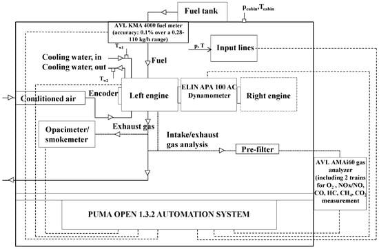
Figure 1.
Scheme of the test bench and related instrumentation [].
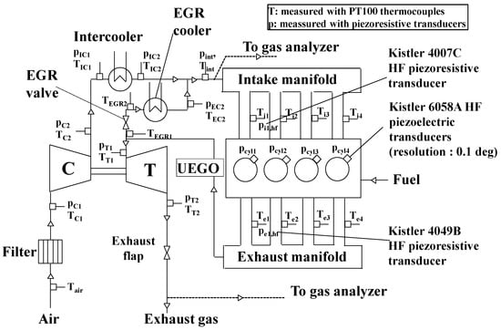
Figure 2.
Scheme of the engine and related instrumentation [].
The engine is equipped with a short-route (high-pressure) cooled EGR system. The EGR valve is placed on the exhaust side, upstream of the cooler. A flap located downstream of the turbine enables both increasing EGR, when the system differential pressure is insufficient, and controlling the exhaust-gas temperature entering the aftertreatment system.
Temperature and low-frequency pressure sensors were installed at several locations as shown in Figure 2. In addition, pressure was measured in all four cylinders using Kistler 6058A high-frequency piezoelectric transducers to obtain in-cylinder pressure–crank-angle data with a resolution of 0.1° CA. The installation of a high-frequency Kistler 4007C piezoresistive sensor in the runner of cylinder 1 allowed the referencing of the in-cylinder pressure signals.
As shown in Figure 1, other instrumentation present in the test rig included an AVL KMA 4000 fuel meter (accuracy 0.1%), an AVL AMA i60 for measuring raw gaseous emissions in the engine exhaust, and an AVL 415S smoke meter providing soot measurements under steady-state conditions. The AVL PUMA OPEN 1.3.2 automation system controlled all the instrumentation.
The experimental tests acquired at the test rig were used preliminarily to calibrate the real-time models implemented in the combustion controller []. These tests consisted of Figure 3:
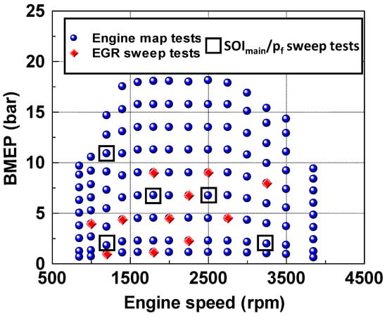
Figure 3.
Summary of the experimental tests [].
- A complete steady-state map consisting of 123 engine points.
- EGR-sweep tests at fixed engine key points, comprising 162 acquisitions. By setting different levels of trapped air mass, with steps of 50 mg/cycle, it was possible to regulate the EGR rate from 0 to 50%.
- sweeps of other relevant quantities, such as the injection timing of the main pulse (SOImain) and injection pressure (pf) at fixed key points comprising 125 acquisitions. Variations of ±6° and ±20% around the nominal values were considered for SOImain and pf, respectively. The implemented injection strategy was a double-injection strategy (pilot + main), in which the pilot quantity and the dwell time between the pilot and main shots were kept constant. During the tests, the rig control system was set to “BMEP-control” mode, so that the test-rig controller could adjust the fuel quantity in the main pulse to maintain BMEP at the desired target.
Conventional diesel fuel (in accordance with EN 590 []), whose main properties are reported in Table 2, was used for all the tests.
Table 2.
Main properties of the diesel fuel used in the tests [].
3. Materials and Methods
The proposed methodology is based on a previously developed low-throughput combustion model, which is able to simulate the heat release on the basis of the accumulated fuel mass approach and the in-cylinder pressure trace on the basis of a single-zone thermodynamic model. In this study, the combustion model has also been refined with respect to the previous version in order to better capture the in-cylinder pressure trace during the blowdown phase and to make it capable of estimating the exhaust manifold temperature. The model is described in Section 3.1.
A genetic algorithm-based optimizer has been used to adjust the main model calibration parameters in order to minimize objective functions, which take into account the prediction error of BMEP, PFP, IMEP360, MFB50 and Texh.
Three different scenarios have been considered in this study:
Scenario 1: no in-cylinder sensors. No pressure transducers are installed. The objective function of the GA optimizer only includes the prediction errors of BMEP and Texh, two quantities which are commonly measured during experimental activities.
Scenario 2: sensors used but only indicated quantities stored. Pressure sensors are available during the campaign but only cycle-averaged indicated quantities (i.e., PFP, IMEP360 and MFB50) are considered, rather than crank-angle-resolved data. Therefore, the objective function is based on the prediction errors of these quantities. This scenario is useful to assess the accuracy in the prediction of heat release and in-cylinder pressure traces when the model is tuned using only cycle-averaged indicated data, which are generally stored together with time-averaged quantities in a low-frequency output data file.
Scenario 3: combined signals. This case investigates a combination of scenario 1 and scenario 2, so that the objective function includes the prediction errors of BMEP, PFP, MFB50 and Texh. IMEP360 was not used since it is closely correlated to BMEP.
The optimizer is described in Section 3.2.
3.1. Low-Throughput Combustion Model
The detailed description of the combustion model can be found in [] and its scheme is described in Figure 4.
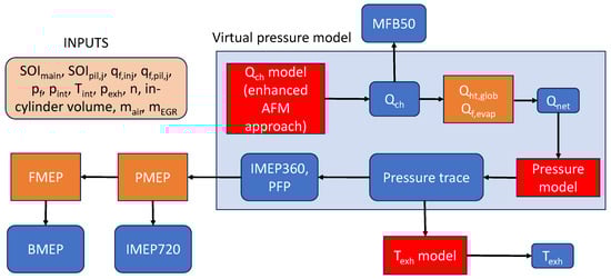
Figure 4.
Scheme of the combustion model.
The model includes the simulation of:
- Heat release: the chemical energy release is estimated with a model based on the accumulated fuel mass approach that uses the fuel injection rate as input.
- In-cylinder pressure: the calculation adopts a single-zone approach and requires the net energy release Qnet. This quantity is derived from the chemical energy release, by accounting for heat transfer and fuel evaporation effects (Qht,glob, Qf,evap). The gross IMEP (IMEP360) and PFP are obtained from the in-cylinder pressure trace.
- Pumping losses: the pumping mean effective pressure (PMEP) was evaluated using a semi-empirical correlation that depends on the intake and exhaust manifold pressure levels, and on the engine speed. The PMEP is used to derive the net IMEP (i.e., IMEP720) starting from IMEP360.
- Friction losses: the Chen–Flynn approach [] has been used to predict FMEP on the basis of the engine speed and peak firing pressure.
- Exhaust manifold temperature: a semi-empirical model has been introduced in this study to evaluate the exhaust manifold temperature, on the basis of the simulated in-cylinder pressure.
A short description of the model is reported in this study. However, the reader may refer to [,] for further details.
The main equations of the model for the estimation of the chemical energy release (Qch) are reported in Table 3, where the tuning parameters are highlighted in red.
Table 3.
Main equations of the chemical energy release model [].
In Table 3, j indicates the generic injection pulse, HL is the fuel lower heating value, K and τ are the combustion rate and ignition delay coefficients of the Qch model. The quantity is the fuel injection rate, which is modeled on the basis of injection data (fuel injection quantities, timings, energizing time and injection pressure). The injection rate of each pulse is the main input of the model.
The next step consists in evaluating the net energy release curve, by means of the approach reported in Table 4, taking into account heat transfer and fuel evaporation effects.
Table 4.
Main equations of the net energy release model [].
In Table 4, Qf,evap and Qht,glob are calibration parameters and indicate the fuel evaporation heat from SOI to SOC (J) and the heat exchanged by the charge with the walls over the combustion cycle (J), respectively. is the total injected fuel mass per cyc/cyl. As can be seen, the net energy release is obtained by scaling the chemical energy release curve according to the global heat exchanged with the walls, and then subtracting the fuel evaporation heat.
Subsequently, the in-cylinder pressure model is estimated on the basis of the equations reported in Table 5.
Table 5.
Main equations of the in-cylinder pressure model [].
In Table 5, pint indicates the intake manifold pressure, pexh the exhaust manifold pressure, pIVC the in-cylinder pressure at IVC, m and m′ the compression and expansion polytropic exponents. Tuning parameters have been highlighted in red.
Figure 5 shows the different intervals in which the pressure is modeled.
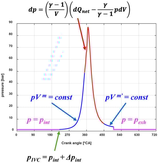
Figure 5.
In-cylinder pressure estimation.
Basically, it can be seen that during the intake and discharge phases, the pressure in the chamber is set equal to the intake manifold and exhaust manifold pressure, respectively. At IVC the in-cylinder pressure is set equal to the intake manifold pressure plus an adjustment parameter Δpint. During the compression and expansion phases, polytropic evolutions are assumed, while during the combustion phase the pressure is obtained by means of a single zone approach [].
The previous version of the pressure model had originally been developed for combustion control applications [], and therefore some simplifications were performed, such as assuming the in-cylinder pressure to be equal to the exhaust manifold during the blowdown and gas discharge phase. It was verified that this assumption can lead to non-negligible errors in the estimation of IMEP and BMEP, therefore a novel approach has here been introduced.
In particular, an exponential equation has been used, as follows:
The previous equation is used to estimate the in-cylinder pressure in the interval between the exhaust valve opening (EVO) and the end of cycle. The pressure computed by this relation tends to pexh for high values of θ. The coefficients of the equation were tuned on the basis of the available experimental dataset, and they are equal to a = 1.68, b = 50° CA, c = 0.8, θEVO = 500° CA.
Figure 6 shows, for four selected operating conditions of the engine map (including high/low speed and load conditions), a comparison between the experimental pressure trace (blue line), the predicted pressure trace with the original model developed in [] (green line) and the improved model using Equation (14) (red line) in the blowdown interval after the exhaust valve opening.
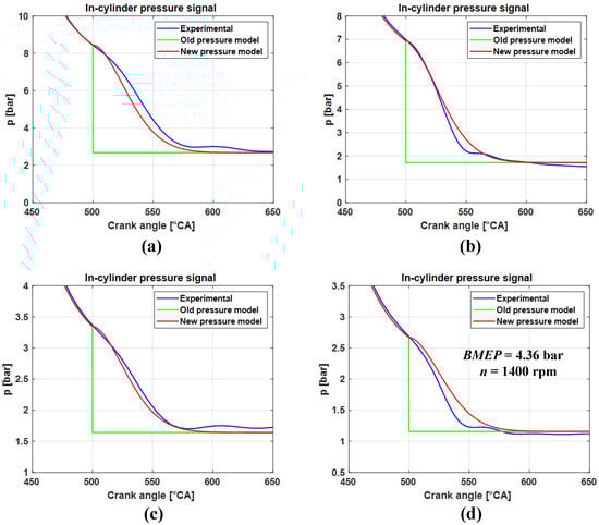
Figure 6.
Comparison between the experimental pressure trace (blue line), the predicted pressure trace with the original model developed in [] (green line) and the improved model using Equation (14) (red line) in the blowdown interval after the exhaust valve opening. Four operating points are examined: 15.08 bar x 3000 rpm (a), 15.25 bar x 1400 rpm (b), 4.31 bar x 3000 rpm (c) and 4.36 bar x 1400 rpm (d).
As shown, the new approach accurately captures the blowdown phase, leading to a better prediction of the in-cylinder pressure trace.
As far as friction and pumping losses are concerned, they were estimated by the following engine-dependent equations (see []):
Finally, a semi-empirical approach has been introduced in this study to estimate the exhaust manifold gas temperature.
The method starts from the evaluation of the in-cylinder temperature at exhaust valve opening (TEVO) on the basis of the following relation, which derives by applying the first law of the thermodynamics to the in-cylinder content:
where TIVC was assumed equal to the intake manifold temperature, qf,inj is the injected fuel volume, ρLHV is the product of the fuel density by the fuel’s lower heating value, cV is the specific heat at constant volume, mair and mEGR are the mass of air and EGR.
Once TEVO is known, the following semi-empirical correlation is used to estimate the exhaust manifold temperature from TEVO:
It was verified that the previous correlation is very robust over the entire dataset, and only the pre-multiplying coefficient is engine dependent. This can be seen in Figure 7, which compares the predicted and experimental values of the exhaust manifold temperature for the engine considered in this study (Figure 7a) and for an 11 L diesel engine (refer to []):
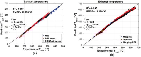
Figure 7.
Comparison between the predicted and experimental values of Texh for the 3 L engine considered in this study (a) and for the 11 L engine considered in [] (b).
3.2. Genetic Algorithm-Based Optimizer
A genetic algorithm (GA) optimizer was used in a Matlab environment for the combustion model tuning (Matlab® R2024b was used). The optimizer, for each operating condition, adjusts a set of the combustion model parameters in order to minimize a weighted objective function (fobj). As previously reported, three different scenarios have been considered, which are defined by the following objective functions:
In Equation (20) the gross value of IMEP (i.e., IMEP360) is used, to avoid the need to estimate pumping losses.
It can be observed that equal weights were assigned to scenarios 2 and 3, which were found to yield satisfactory results, whereas, for scenario 1, the optimal configuration involved assigning a higher weight to Texh than to BMEP. This aspect will be further examined in the Section 4. In the previous equations, the relative prediction errors of BMEP, IMEP360, PFP, MFB50 and Texh were used. For a generic quantity ‘X’, the relative prediction error is defined as follows:
where the experimental quantities are indicated by the subscript ‘exp’. A subset of the combustion model parameters was selected for calibration, i.e., those shown to have the greatest influence on the prediction of heat release and in-cylinder pressure. The remaining parameters were held constant at mean values or obtained from correlations in the literature, such as the ignition delay of the main and pilot injections.
Table 6 reports, in red, the model parameters that were used for model calibration in the GA optimizer, along with their variation range for the optimization. Instead, the parameters that were not used for model tuning are indicated in black.
Table 6.
model parameters that were used in the GA optimizer (parameters used for model calibration are indicated in red, parameters not used for model calibration are indicated in black).
The genetic algorithm is a population-based optimization method inspired by natural selection. An initial random population of Ni individuals is generated and evolved for Ng generations using mutation and crossover operators. Individuals are ranked by the objective function; those with the lowest objective values are considered the best ones.
In this study, the population size has been set to 200, in order to provide sufficient degrees of freedom for the genetic algorithm.
The maximum number of generations has been set equal to 1000, to give the mutation process more opportunities to improve solution quality. A further refinement has been provided by setting the maximum number of stall generations to 500. This parameter imposes the maximum number of generations where no significant improvement in the objective function minimization is detected.
The default mutation function used when lower and upper boundaries are set for the tuning parameters is the «mutationadaptfeasible». It is a function that randomly generates directions which are adaptive with respect to the last successful or unsuccessful generation. Two parameters can be tuned about this function:
- -
- scale: it is the initial value of the mutation step;
- -
- shrink: it is the reduction factor of the mutation step at each generation. The variation range of this parameter is between 0 and 1. Values of shrink close to 0 cause the mutation step to shrink rapidly, while values near 1 keep the step large for longer.
To investigate the effect of each parameter, values different from the default settings (scale = 1, shrink = 1) were tested. However, no relevant effect has been detected, therefore the default values were left.
The influence of the crossover fraction was also analyzed. This parameter sets the percentage of new solutions which are generated by the crossover operator with respect to the total amount of new individuals created at each generation. The value of 0.2 was selected as the optimal one.
Figure 8 reports the performance of the GA-based optimizer for the three considered objective functions, in terms of the fitness of the best individual (blue) and the average one (orange), as a function of the number of generations. It can be seen that the optimization algorithms converge to a good solution within 50–100 generations, depending on the considered scenario.
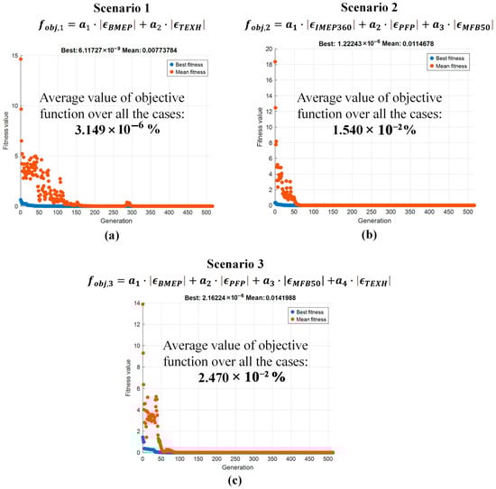
Figure 8.
Performance of the genetic algorithms optimizer for the objective function of scenario 1 (a), scenario 2 (b) and scenario 3 (c).
The average time required by the genetic algorithm is of the order of 25 h for scenario 1 (i.e., 3.6 min per test), 30 h (i.e., 4.4 min per test) for scenario 2 and 40 h for scenario 3 (i.e., 5.8 min per test), when the calculation is performed on a PC with 1.80 GHz i7 processor and 16GB of RAM.
4. Results and Discussion
The methodology explained in Section 3 was applied to the entire available dataset. First, a comparison between the predicted and experimental values of the main combustion and performance metrics is shown for the entire dataset. Subsequently, the predicted and experimental curves of heat release and in-cylinder pressure will be shown for some selected operating conditions.
Figure 9, Figure 10 and Figure 11 show, for the three different scenarios, the predicted vs. experimental values of the BMEP (a), IMEP360 (b), Texh (c), PFP (d), MFB50 (e) and Qnet,max (f).
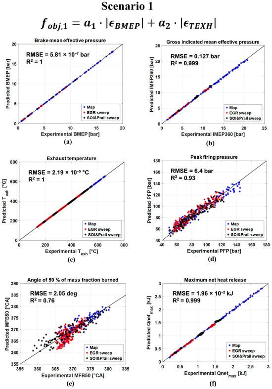
Figure 9.
Predicted vs. experimental values of the BMEP (a), IMEP360 (b), Texh (c), PFP (d), MFB50 (e) and Qnet,max (f) for scenario 1.
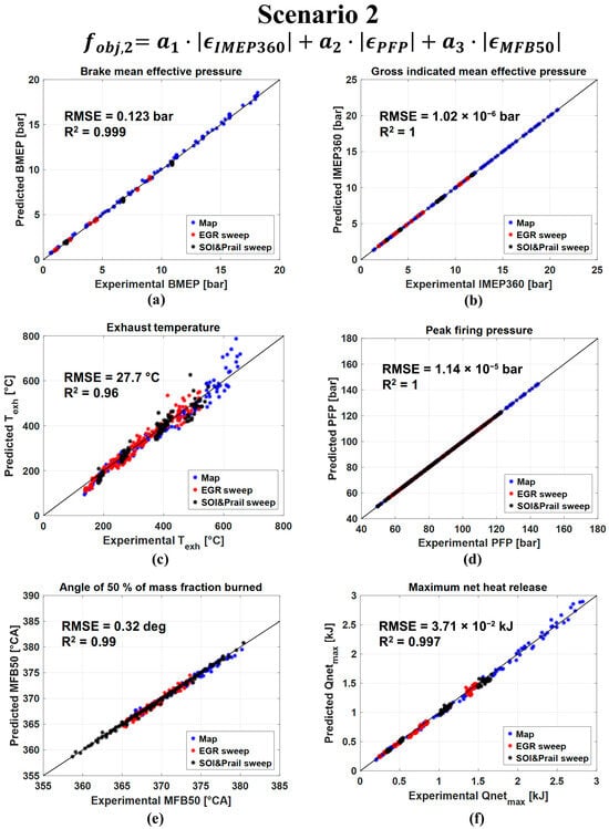
Figure 10.
Predicted vs. experimental values of the BMEP (a), IMEP360 (b), Texh (c), PFP (d), MFB50 (e) and Qnet,max (f) for scenario 2.
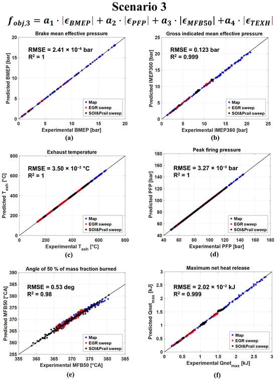
Figure 11.
Predicted vs. experimental values of the BMEP (a), IMEP360 (b), Texh (c), PFP (d), MFB50 (e) and Qnet,max (f) for scenario 3.
In the first scenario, it can be seen that the predicted values of BMEP and Texh match the target values with a very high level of accuracy (R2 is around 1), and this confirms that the GA optimizer has converged to an optimal solution in all cases. In addition, it can be seen that the gross IMEP (i.e., IMEP360) and the maximum value of the net energy release (Qnet,max) are also very well captured, as the value of the correlation coefficient is around 0.99 and the RMSE values are very small, and this suggests that in-cylinder pressure and heat release traces are well predicted. The peak firing pressure is captured with a good level of accuracy (R2 = 0.93, RMSE = 6.4 bar), as well as the MFB50 (R2 = 0.76, RMSE = 2.05 deg). These results confirm that, even without the installation of an in-cylinder pressure sensor, the main metrics related to heat release, in-cylinder pressure and engine performance can be reproduced with a good level of accuracy, just using BMEP and exhaust manifold temperature for tuning.
In the second scenario, it can be observed that the predicted values of IMEP360, PFP and MFB50 match the target values with a high level of accuracy (R2 is around 1), confirming that the GA optimizer has converged to an optimal solution in all cases. BMEP is also well captured (R2 = 0.999, RMSE = 0.123 bar). Also in this case the accuracy in the prediction of Qnet,max is very high, as the value of the correlation coefficient is around 0.99 and the RMSE values are very small, and this suggests that in-cylinder pressure and heat release traces are well captured. A small deterioration of the prediction of Texh is observed, which, however, is still captured with a good level of accuracy (R2 = 0.96, RMSE = 27.7 °C). These results show that using the indicated quantities only (i.e., PFP, IMEP360, MFB50) improves the accuracy in the prediction of the in-cylinder pressure and heat release curves, while also providing a good prediction of the exhaust manifold temperature.
Finally, in the last scenario, the predicted values of BMEP, PFP, MFB50 and Texh match the target values with a high level of accuracy (R2 is around 1), confirming that the GA optimizer has converged to an optimal solution in all conditions. Also in this case IMEP360 and Qnet,max are very well captured, as the value of the correlation coefficient is around 0.99 and the RMSE values are small. This scenario provides the best results in terms of predicting the pressure and the heat release metrics.
Concerning the accuracy in the estimation of the in-cylinder pressure and net heat release curves, four engine operating conditions were selected, which include low/high speed and load conditions.
Figure 12 shows, for the selected operating points and the different scenarios, the experimental and predicted trends of the net heat release, while Figure 13 compares the corresponding in-cylinder pressure traces.
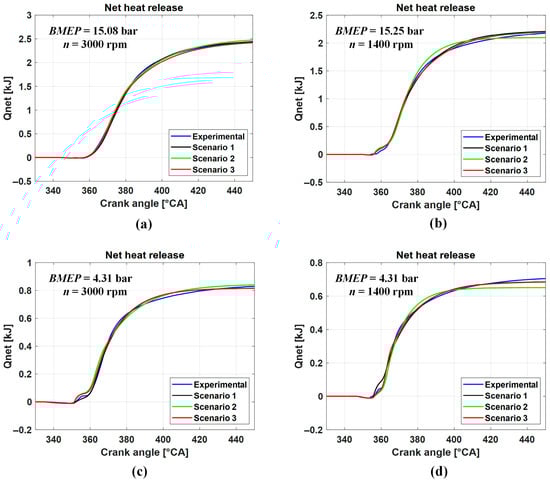
Figure 12.
Experimental and predicted trends of the net heat release for the three different scenarios, considering the four operating points: 15.08 bar x 3000 rpm (a), 15.25 bar x 1400 rpm (b), 4.31 bar x 3000 rpm (c) and 4.36 bar x 1400 rpm (d).
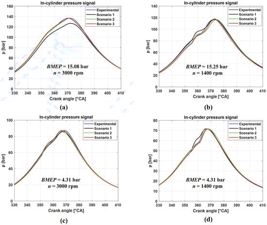
Figure 13.
Experimental and predicted trends of in-cylinder pressure for the three different scenarios, considering the four operating points: 15.08 bar x 3000 rpm (a), 15.25 bar x 1400 rpm (b), 4.31 bar x 3000 rpm (c) and 4.36 bar x 1400 rpm (d).
The results shown in Figure 12 highlight that the model is able to capture the net heat release trends with a very high level of accuracy, not only when the indicated metrics are used for calibration (i.e., scenario 2 and 3), but also when only BMEP and the exhaust manifold temperature are used (scenario 1). This result is particularly interesting and of useful application, since the heat release curves can be predicted with a very high level of accuracy, both in terms of shape and maximum value, even without the use of costly in-cylinder pressure sensors. The good matching of the maximum value of the net heat release curve indicates that heat transfer is very well captured, even in scenario 1 where only BMEP and Texh are used for calibration.
Figure 13 shows that, in general, in-cylinder pressure traces are well captured in almost all cases. A deterioration in accuracy can be observed for the point at n = 3000 rpm and BMEP = 15.08 bar (Figure 13a) for the first scenario. However, the error is in line with the RMSE values shown in Figure 9d. Concerning this engine point, the deterioration seems to be mainly related to a non-optimal prediction of the compression phase, which is due to an underestimation of the polytropic compression exponent, while the combustion phase is well captured. Instead, when the indicated data are available (scenarios 2 and 3), the in-cylinder pressure estimation is very accurate in all cases.
Figure 14 shows the speed and load conditions for each case number. To better evaluate the capability of the method to accurately simulate the curves of net energy release and in-cylinder pressure over the entire dataset, Figure 15 and Figure 16 report the values of R2 and RMSE for the Qnet curve (Figure 15) and for the pressure curve (Figure 16) calculated in the crank angle interval between 330° CA and 450 °C, for the different scenarios. The values are plotted vs. the case number, but the type of test is highlighted (i.e., engine map, EGR sweep and SOI/prail sweep).

Figure 14.
Speed and load conditions as a function of the case number.
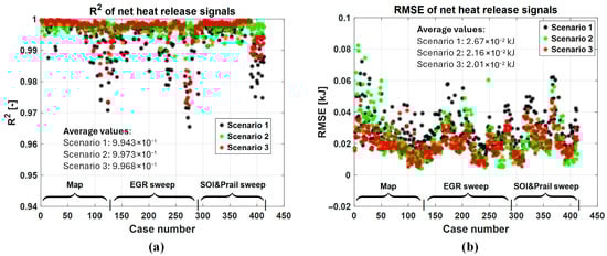
Figure 15.
values of R2 (a) and RMSE (b) calculated on the basis of the predicted and experimental curves of net energy release, in the crank angle interval between 330° CA and 450° CA.
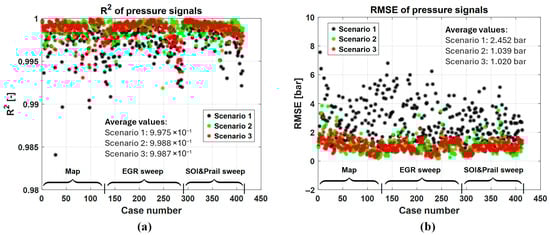
Figure 16.
values of R2 (a) and RMSE (b) calculated on the basis of the predicted and experimental curves of in-cylinder pressure, in the crank angle interval between 330° CA and 450° CA.
Concerning the values of R2 of the net energy release signals, it can be seen that all the scenarios display higher values than 0.96 over the entire dataset, confirming that the correlation between the predicted and experimental trends is very high. With reference to the RMSE values, the best results are obtained in scenarios 2 and 3 (average RMSE values equal to 2.16 × 10⁻² and 2.01 × 10⁻² kJ, respectively), although in scenario 2 larger errors may occur for some operating conditions (i.e., especially for the first 50 points, which correspond to high load engine map conditions, see Figure 14). The good results obtained in scenario 2 suggest that using the cycle-averaged indicated data only (i.e., PFP, IMEP360 and MFB50) is sufficient to obtain a very accurate estimation of the heat release curves. Scenario 1 is also very effective in reproducing the heat release curves with low errors over the entire dataset (RMSE = 2.67 × 10⁻² kJ), and this confirms the robustness of the method, even when no in-cylinder pressure sensors are used.
Concerning the values of R2 of the in-cylinder pressure signals, it can be seen that all the scenarios display higher values than 0.98 over the entire dataset, confirming that the correlation between the predicted and experimental trends is very high. With reference to the RMSE values, the best results are obtained in scenarios 2 and 3 (average RMSE values equal to 1.039 and 1.02 bar, respectively). Also in this case, similarly to the net energy release estimation, larger errors may occur in scenario 2 for some operating conditions (i.e., especially for the first 50 points, which correspond to high load engine map conditions, see Figure 14). However, the results obtained in scenario 2 suggest that using the cycle-averaged indicated data only (i.e., PFP, IMEP360 and MFB50) is sufficient to obtain a very accurate estimation of the in-cylinder pressure curves. When the first scenario is considered, a general deterioration in the prediction of the in-cylinder pressure trace occurs, but the RMSE values are still low (i.e., around 2.45 bar). Therefore, the use of BMEP and exhaust manifold temperature only still provides accurate results.
A final remark has to be made concerning the choice of the weights in the objective functions. While the use of equal weights has brought satisfactory results for scenario 2 and scenario 3, an investigation has been conducted for scenario 1 which displays the least accurate results. In particular, three cases were analyzed, in which the weight factors of Equation (19) are equal to:
- Case 1: a1 = 0.25, a2 = 0.75 (final selected condition)
- Case 2: a1 = 0.5, a2 = 0.5
- Case 3: a1 = 0.75, a2 = 0.25
Table 7 reports, for scenario 1, the effect of the selection of the weights on the values of R2 and RMSE for the prediction of Qnet and in-cylinder pressure curves.
Table 7.
Effect of the selection of the weights on the values of R2 and RMSE for the prediction of Qnet and in-cylinder pressure curves, for scenario 1.
It can be seen that, in general, the effect of the weight selection is small. However, a slight improvement of the accuracy of the prediction of the Qnet and in-cylinder pressure traces can be seen for case 1, which has been selected as the optimal one.
5. Final Considerations and Future Work
The proposed methodology was demonstrated to be effective in estimating the heat release rate and in-cylinder pressure from basic testbed data for all the considered scenarios. Moreover, the combustion model is low-throughput, making it straightforward for other researchers to implement and reproduce results on different engines, including those operating on alternative fuels, because the approach is fuel-independent.
In this study, the method was applied considering hot test conditions. However, it can potentially be applied also to cold start conditions, if the corresponding experimental values of BMEP, MFB50, PFP, IMEP360 and Texh are provided. Potential limitations could emerge when applying the method in large transient conditions, concerning the use of the exhaust manifold temperature as an input variable. In fact, due to the dynamic response of the temperature sensor, a time delay may occur between the combustion cycle and the corresponding value of Texh measured by the sensor. Therefore, this may affect the accuracy of the method in the scenarios in which Texh is used (i.e., scenario 1 and scenario 3), while scenario 2 is expected to be more robust, since it is just based on cycle-averaged indicated quantities (i.e., PFP, MFB50, IMEP360).
Future work will include the development of alternative strategies for in-cylinder estimation (such as neural networks and artificial intelligence-based methods) and the comparison with the method proposed in this study. The authors will also seek physically consistent correlations for the key parameters of the combustion model, based on the test-by-test calibrations reported here, and will rigorously assess the accuracy of the resulting calibrated model.
6. Conclusions
A methodology for the estimation of the in-cylinder pressure and heat release in diesel engines from basic testbed measurements was proposed. The method exploits a previously developed low-throughput combustion model, which can predict the heat release and in-cylinder pressure curves, and which has been further refined in this study to simulate more accurately the blowdown phase and to evaluate the exhaust manifold temperature. A genetic algorithm was adopted to tune the combustion model using basic testbed data which are commonly measured. These data are the brake mean effective pressure (BMEP), the gross indicated mean effective pressure (IMEP360), the peak firing pressure (PFP), the crank angle at which 50% of fuel mass has burnt (MFB50) and the exhaust gas temperature (Texh). Three different scenarios were considered, in which different subsets of the three previous quantities were assumed to be known. The first scenario assumes that no pressure transducers are installed in the engine, so that the model is tuned for minimizing the prediction errors of BMEP and Texh only. In the second scenario, it was assumed that indicated quantities only (i.e., PFP, IMEP360 and MFB50) are available. The third scenario, finally, assumes that BMEP, PFP, MFB50 and Texh are available.
It was verified that, in general, the heat release curve and the in-cylinder pressure are accurately simulated over the entire dataset for all the three considered scenarios. In fact, for the net energy release curve the RMSE values are of the order of 2.67 × 10⁻² kJ, 2.2 × 10⁻² kJ and 2.0 × 10⁻² kJ for the three scenarios, respectively, while the RMSE values for the in-cylinder pressure curves are around 2.45 bar, 1.04 bar and 1.02 bar, respectively. The slight deterioration observed in the first scenario is, however, acceptable, considering that in this case no indicated quantities are used for model tuning (i.e., only BMEP and Texh are used).
The approach proposed in this study for heat release and in-cylinder pressure simulation has several advantages.
First, it adopts a physically consistent combustion model rather than a black-box solution, so that it is expected to be more robust outside the calibration range. Moreover, the combustion model is of the low-throughput type, therefore it requires a low computational effort. On the one hand, this allows large datasets to be processed with computational times on the order of some hours, since the computational time required to elaborate a single condition ranges between 3.6 min and 5.8 min depending on the scenario. On the other hand, the low-throughput nature of the model also makes it straightforward for other researchers to implement and reproduce results on different engines. It should also be noted that the method is fuel-independent and can be applied to engines running on conventional diesel or on alternative/zero-carbon fuels, which are currently being extensively studied as potential ways to reduce the environmental impact of internal combustion engines. Finally, another advantage is that model calibration does not rely on dynamic signals which require dedicated sensors (such as the instantaneous engine speed), but only on standard testbed measurements which are commonly acquired.
Future steps will include the assessment of different engines, the exploration of alternative methodologies, such as artificial intelligence-based approaches, and the identification of physically consistent correlations for the tuning parameters of the model, based on the dataset identified in this study.
Author Contributions
Conceptualization, R.F.; Methodology, R.F.; Software, F.G., Formal Analysis, R.F., S.d., F.G.; Data Curation, R.F., S.d., F.G.; Writing—Original Draft Preparation, R.F., S.d., F.G.; Writing—Review and Editing, R.F., S.d., F.G.; Supervision, R.F., S.d. All authors have read and agreed to the published version of the manuscript.
Funding
This research received no external funding.
Data Availability Statement
The original contributions presented in this study are included in the article. Further inquiries can be directed to the corresponding author.
Acknowledgments
Omar Marello is acknowledged for the support.
Conflicts of Interest
The authors declare no conflicts of interest.
Abbreviations
The following abbreviations are used in this manuscript:
| ANN | Artificial neural network |
| BMEP | Brake Mean Effective Pressure (bar) |
| CA | crank angle (deg) |
| ECU | Engine Control Unit |
| EGR | Exhaust Gas Recirculation |
| EOC | End of combustion |
| EVO | Exhaust Valve Opening |
| FMEP | Friction Mean Effective Pressure (bar) |
| GA | Genetic algorithm |
| HL | Fuel lower heating value |
| HVO | Hydrotreated Vegetable Oil |
| ICE | Internal Combustion Engine |
| IMEP | Indicated Mean Effective Pressure (bar) |
| IMEP360 | net Indicated Mean Effective Pressure (bar) |
| IMEP720 | gross Indicated Mean Effective Pressure (bar) |
| IVC | Intake Valve Closing |
| m | mass |
| MFB50 | crank angle at which 50% of the fuel mass fraction has burned (deg) |
| MPC | Model predictive control |
| n | engine rotational speed (1/min) |
| p | pressure (bar) |
| pexh | exhaust manifold pressure (bar abs) |
| pf | injection pressure (bar) |
| PFP | peak firing pressure |
| pint | intake manifold pressure (bar abs) |
| PM | Particulate matter |
| PMEP | Pumping Mean Effective Pressure (bar) |
| q | injected fuel volume quantity (mm3) |
| Qch | chemical energy release |
| qf,inj | total injected fuel volume quantity per cycle/cylinder |
| Qnet | net heat release |
| RMSE | root mean square error |
| SCR | selective catalytic reduction |
| SOC | Start of combustion |
| SOI | electric start of injection |
| SOImain | electric start of injection of the main pulse |
| T | temperature (K) |
| TDC | Top dead center |
| Texh | exhaust manifold temperature |
| Tint | intake manifold temperature |
| V | volume |
| V2I | Vehicle-to-infrastructure |
| V2V | Vehicle-to-vehicle |
| VGT | Variable geometry turbocharger |
References
- Euro 7: Council Adopts New Rules on Emission Limits for Cars, Vans and Trucks. Available online: https://www.consilium.europa.eu/en/press/press-releases/2024/04/12/euro-7-council-adopts-new-rules-on-emission-limits-for-cars-vans-and-trucks/ (accessed on 24 September 2025).
- d’Ambrosio, S.; Mancarella, A.; Manelli, A. Utilization of Hydrotreated Vegetable Oil (HVO) in a Euro 6 Dual-Loop EGR Diesel Engine: Behavior as a Drop-In Fuel and Potentialities along Calibration Parameter Sweeps. Energies 2022, 15, 7202. [Google Scholar] [CrossRef]
- Mancarella, A.; Marello, O. Effect of Coolant Temperature on Performance and Emissions of a Compression Ignition Engine Running on Conventional Diesel and Hydrotreated Vegetable Oil (HVO). Energies 2023, 16, 144. [Google Scholar] [CrossRef]
- Jaworski, A.; Kuszewski, H.; Szpica, D.; Woś, P.; Balawender, K.; Ustrzycki, A.; Krzemiński, A.; Jakubowski, M.; Mieczkowski, G.; Borawski, A.; et al. Comparative Study on the Effects of Diesel Fuel, Hydrotreated Vegetable Oil, and Its Blends with Pyrolytic Oils on Pollutant Emissions and Fuel Consumption of a Diesel Engine Under WLTC Dynamic Test Conditions. Energies 2025, 18, 5038. [Google Scholar] [CrossRef]
- Milojević, S.; Stopka, O.; Kontrec, N.; Orynycz, O.; Hlatká, M.; Radojković, M.; Stojanović, B. Analytical Characterization of Thermal Efficiency and Emissions from a Diesel Engine Using Diesel and Biodiesel and Its Significance for Logistics Management. Processes 2025, 13, 2124. [Google Scholar] [CrossRef]
- Kabudke, P.D.; Kharde, Y.R.; Parkhe, R.A. Experimental investigation on performance of cotton seed biofuel blended with diesel on variable compression ratio diesel engine. Mater. Today Proc. 2023, 72, 846–852. [Google Scholar] [CrossRef]
- Patel, S.; Torgal, S.; Purohit, T.; Kumar, R.; Singh, D.V.; Kanchan, S.; Soudagar, M.E.M.; Ahamad, T.; Kalam, M.A.; Patel, M. Impact of variable exhaust valve timing on diesel engine characteristics fueled with waste cooking oil biofuel blends: A numerical analysis. In Proceedings of the Institution of Mechanical Engineers, Part E: Journal of Process Mechanical Engineering, London, UK, 11 August 2023; Volume 239, pp. 1329–1352. [Google Scholar] [CrossRef]
- Xing, S.; Li, X.; Li, J.; Gao, J.; Lu, Q.; Wang, X.; Zhao, Y.; Wu, S.; Fu, Z. Numerical Study and Optimization of Combustion and Emissions of Ammonia/Diesel Dual-Fuel Engines Under Heavy Load. Energies 2025, 18, 4841. [Google Scholar] [CrossRef]
- Tutak, W.; Jamrozik, A. Analysis of the Application of Ammonia as a Fuel for a Compression-Ignition Engine. Energies 2025, 18, 3217. [Google Scholar] [CrossRef]
- Shi, X.; Xiong, Q.; Wang, H.; Han, K.; Liu, L.; Pan, C.; Zhao, J. Innovative method of in-cylinder purification emission control in low-speed marine engines: Numerical study on ammonia/diesel high-pressure direct injection. Appl. Therm. Eng. 2025, 267, 125769. [Google Scholar] [CrossRef]
- Scrignoli, F.; Pisapia, A.M.; Savioli, T.; Mancaruso, E.; Mattarelli, E.; Rinaldini, C.A. Exploring Hydrogen–Diesel Dual Fuel Combustion in a Light-Duty Engine: A Numerical Investigation. Energies 2024, 17, 5761. [Google Scholar] [CrossRef]
- Chen, Z.; Ju, P.; Wang, Z.; Shi, L.; Deng, K. Research on multi-objective optimization control of diesel engine combustion process based on model predictive control-guided reinforcement learning method. Energy 2025, 325, 136173. [Google Scholar] [CrossRef]
- Gu, J.; Wang, Y.; Hu, J.; Zhang, K.; Shi, L.; Deng, K. Real-time prediction of fuel consumption and emissions based on deep autoencoding support vector regression for cylinder pressure-based feedback control of marine diesel engines. Energy 2024, 300, 131570. [Google Scholar] [CrossRef]
- Foglia, A.; Cervone, D.; Frasci, E.; Arsie, I.; Pianese, C.; Polverino, P. Model based combustion control optimization of compression ignition engine fuelled with Diesel/OMEx blends. IFAC-PapersOnLine 2025, 59, 127–132. [Google Scholar] [CrossRef]
- Van Dooren, S.; Amstutz, A.; Onder, C.H. A causal supervisory control strategy for optimal control of a heavy-duty Diesel engine with SCR aftertreatment. Control Eng. Pract. 2022, 119, 104982. [Google Scholar] [CrossRef]
- Wassén, H.; Dahl, J.; Idelchi, A. Holistic diesel engine and exhaust after-treatment model predictive control. IFAC-PapersOnLine 2019, 52, 347–352. [Google Scholar] [CrossRef]
- Heywood, J.B. Internal Combustion Engine Fundamentals; McGraw-Hill Intern: Columbus, OH, USA, 1988. [Google Scholar]
- Finesso, R.; Hardy, G.; Marello, O.; Spessa, E.; Yang, Y. Model-Based Control of BMEP and NOx Emissions in a Euro VI 3.0L Diesel Engine. SAE Int. J. Engines 2017, 10, 2288–2304. [Google Scholar] [CrossRef]
- d’Ambrosio, S.; Di Dio, C.; Finesso, R. Model-Based Calibration and Control of Tailpipe Nitrogen Oxide Emissions in a Light-Duty Diesel Engine and Its Assessment through Model-In-The-Loop. Energies 2023, 16, 8030. [Google Scholar] [CrossRef]
- Mansfield, A.B.; Chakrapani, V.; Li, Q.; Wooldridge, M.S. Genetic Optimization for Engine Combustion System Calibration: A Case Study of Optimization Performance Sensitivity to Algorithm Search Parameters. ASME J. Energy Resour. Technol. 2022, 144, 82308. [Google Scholar] [CrossRef]
- Vossoughi, G.R.; Rezazadeh, S. Optimization of the Calibration for an Internal Combustion Engine Management System Using Multi-Objective Genetic Algorithms. In Proceedings of the 2005 IEEE Congress on Evolutionary Computation, Edinburgh, UK, 2–5 September 2005. [Google Scholar] [CrossRef]
- Cruz-Peragon, F.; Jimenez-Espadafor, F. A Genetic Algorithm for Determining Cylinder Pressure in Internal Combustion Engines. Energy Fuels 2007, 21, 2600–2607. [Google Scholar] [CrossRef]
- Mehnatkesh, H.; Gordon, D.; Koch, C.R. Physics-Informed Neural Networks for In-Cylinder Pressure Prediction in Hydrogen/Diesel Dual-Fuel Engines. IFAC-PapersOnLine 2025, 59, 7–12. [Google Scholar] [CrossRef]
- Kekez, M.; Ambrozik, A.; Radziszewski, L. Modeling of Cylinder Pressure in Compression Ignition Engine with Use of Genetic-Fuzzy System Part 1: Engine Fueled by Diesel Oil. Diagnostyka 2008, 4, 9–12. Available online: https://bibliotekanauki.pl/articles/329046.pdf (accessed on 1 October 2025).
- Finesso, R.; Hardy, G.; Maino, C.; Marello, O.; Spessa, E. A New Control-Oriented Semi-Empirical Approach to Predict Engine-Out NOx Emissions in a Euro VI 3.0 L Diesel Engine. Energies 2017, 10, 1978. [Google Scholar] [CrossRef]
- BS EN 590:2022; Automotive Fuels—Diesel—Requirements and Test Methods. BSI: London, UK, 2022. [CrossRef]
- Chen, S.; Flynn, P. Development of a Single Cylinder Compression Ignition Research Engine; SAE Technical Paper 650733; 1965. Available online: https://www.sae.org/papers/development-a-single-cylinder-compression-ignition-research-engine-650733 (accessed on 1 October 2025). [CrossRef]
- Finesso, R.; Spessa, E.; Yang, Y. Development and Validation of a Real-Time Model for the Simulation of the Heat Release Rate, In-Cylinder Pressure and Pollutant Emissions in Diesel Engines. SAE Int. J. Engines 2016, 9, 322–341. [Google Scholar] [CrossRef]
- Finesso, R.; Hardy, G.; Mancarella, A.; Marello, O.; Mittica, A.; Spessa, E. Real-Time Simulation of Torque and Nitrogen Oxide Emissions in an 11.0 L Heavy-Duty Diesel Engine for Model-Based Combustion Control. Energies 2019, 12, 460. [Google Scholar] [CrossRef]
Disclaimer/Publisher’s Note: The statements, opinions and data contained in all publications are solely those of the individual author(s) and contributor(s) and not of MDPI and/or the editor(s). MDPI and/or the editor(s) disclaim responsibility for any injury to people or property resulting from any ideas, methods, instructions or products referred to in the content. |
© 2025 by the authors. Licensee MDPI, Basel, Switzerland. This article is an open access article distributed under the terms and conditions of the Creative Commons Attribution (CC BY) license (https://creativecommons.org/licenses/by/4.0/).