Abstract
This study investigates the effects of high levels of photovoltaic (PV) generation on the unbalanced distribution network using the quasi-dynamic simulation method on DIgSILENT PowerFactory. We are motivated by the need to diversify the national energy matrix, following the power blackout that occurred in Ecuador in 2024 and the energy limitations characterized by the use of fossil fuels. For this purpose, we deployed the simulation of the PJM 13-Node Test Feeder, which is a low-voltage distribution network and mimics the U.S. system, and represents a realist distribution network with residential and commercial load profiles. We simulated realistic PV generation dynamics for a typical day, capturing stochastic solar irradiance, ambient temperature variation, and the impacts of cloud cover. In those conditions, PV generation reached 31.6% of the system total load. We found that during peak irradiance hours, the voltage levels on certain nodes, predominantly low-load buses, exceed nominal levels. The average power factor is noted to diminish by 0.90 p.u to 0.82 p.u at the feeder bus, and further drops to 0.35 p.u at the most PV-penetrated site. While distributed PV generation can effectively reduce line loading and improve energy efficiency, without reactive power compensation, the highest penetration PV generation scenario could result in deterioration of voltage stability and power quality. The prescribed quasi-dynamic framework is practical and computationally feasible, allowing for the assessment of operational performance of distribution networks with high renewables penetration.
1. Introduction
During 2024, Ecuador faced a severe energy crisis caused by climatic factors, low investment, and insufficient maintenance of the electrical power system (EPS). Low rainfall reduced generation from the main hydroelectric plants, resulting in power outages of up to 14 h per day in several sectors. In 2023, the annual electricity demand growth rate reached 9.6%, far exceeding the historical average of 4% per year. To meet electricity demand, the Paute Integral complex, comprising the Mazar, Molino, and Sopladora hydroelectric power plants, contributed 34.1% of the total. In contrast, the Coca Codo Sinclair hydroelectric power plant contributed 29.2% [1]. Figure 1 shows the country’s cumulative annual demand curve for 2024, with a maximum of 5104 MW [2]. According to the latest Electricity Master Plan, 58.7% of generation comes from hydroelectric sources [1]. However, during the same year, the Paute Integral complex was at risk of operation due to low reservoir levels caused by one of the most severe droughts in the last 61 years.
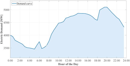
Figure 1.
Annual cumulative demand curve for Ecuador, illustrating the characteristic daily load behavior, with demand reaching its minimum during early morning hours and increasing sharply toward a pronounced evening peak.
Given this background, Ecuador’s EPS faced operational limitations, forcing both residential and commercial users to rely on combustion generators or PV panels. As a result, there was a significant increase in the installation of solar panels as an alternative for generating electricity. This solution helps mitigate the generation deficiency; however, it is necessary to analyze how it could affect the electrical grid’s performance once the drought ends and the system returns to normal operation.
PV has become a viable solution to rising electricity demand. It is estimated that this type of generation, together with other renewable sources (wind, hydro, etc.), will account for 86% of total electricity produced worldwide by 2050 [3]. Although PV generation diversifies the energy matrix, its widespread adoption introduces research challenges due to instabilities inherent in its technological limitations. Unlike synchronous generators, PV generation systems lack an inertial response, and are incapable of providing the necessary contingencies to support and stabilize the system [4,5,6].
PV integration has become a common practice globally, driven in particular by the growing demand for clean energy sources as alternatives to fossil fuels. PVs offer technical benefits, including reduced transmission and distribution losses, increased system resilience, lower generation costs, and reduced need for conventional capacity expansion. However, their large-scale integration must be carefully considered to avoid effects on the stability and security of the electrical system [7].
Scientific literature examines the effect of PV integration on electrical systems. For example, Ref. [8] analyzes the western electrical system of the Democratic Republic of Congo, with a base capacity of 2012 MW, under different PV penetration levels. The study assessed active power loss, voltage stability, and harmonics, among other indicators. The study found that PV generation between 10 percent and 20 percent insertion levels reduced losses, without compromising operational stability. However, above 30 percent, the system experienced technical degradation, manifested in increased voltage oscillations and harmonic distortion due to the low inertia of inverter technology. The study recommends using harmonic filters, storage systems, STATCOM, and other support devices to maintain system reliability.
In [9], it was demonstrated that PV insertion generally improves voltage stability, although its location negatively affects voltage levels. In addition, other studies have shown that excessive PV integration can cause bidirectional power flow problems and voltage instability; however, these issues can be mitigated through reactive power support from the photovoltaic inverter [10,11].
Ref. [12] reviews methods to assess the effects of high PV penetration on power quality indices. The review analyzed a number of deterministic and stochastic approaches, noting that the latter offers a more accurate description of the behavior of the electrical system by factoring in the variability of solar generation. The review describes voltage regulation as the principal technical challenge, even at low levels of PV penetration, stating that the higher levels can cause a multiplicity of power quality issues. In addition, Ref. [13] pointed out that the integration of large-scale PV systems requires contemporary electrical systems to develop new control mechanisms because of its power quality effects and the reduction in system inertia. Therefore, under conditions of high PV penetration, smart control, and battery storage are required to stabilize the system.
On the other hand, Ref. [14] conducted a detailed review of the impacts of high PV penetration on the reliability and stability of electrical systems. The study covered effects on voltage, frequency, harmonic distortion, protections, and flexibility requirements. The study highlights the critical characteristics of PV systems that condition their effective integration into electrical grids.
Voltage stability is a key challenge in large-scale PV integration, defined as the ability of an EPS to maintain all nodes within operational voltage limits under normal and post-disturbance conditions [15]. Stability challenges have been documented as one of the primary factors contributing to the increased prevalence of blackouts in the world [15,16]. In this regard, the behavior of the system is significantly influenced by the location of the distributed generation sources; when distributed resources are poorly sited, the risk of unstable voltage conditions in the locality or the system as a whole is heightened [17,18]. Therefore, it is crucial to consider not just the amount of generation to be injected, but the point of interconnection in the network.
Real power strongly influences voltage stability, since changes in its magnitude or injection method affect the voltage response. This is of greater importance when the power generation source is stochastic, such as photovoltaic systems or wind power, as they are reliant on external conditions that fluctuate. This is why study [19] suggests the analysis of the coordinated control of real and reactive power as a means of keeping voltage in a given operational band.
Many studies address PV integration into electrical systems, but analyzing the system from a quasi-dynamic perspective is necessary to capture the time evolution of the grid under step-wise PV injection. Hence, this article proposes a quasi-dynamic analysis of a 13-node IEEE test system in order to capture the behavior of the electrical grid over the entire day when active power generated from photovoltaics is injected.
The article is structured as follows: after the introduction, Section 2 describes the materials and methods used for this research. Section 3 presents the case studies, while the results and discussions are presented in Section 4. Finally, Section 5 presents the conclusions, emphasizing the most relevant aspects of the simulation results.
2. Materials and Methods
Photovoltaic systems rely directly on solar irradiance, resulting in temporal variability of energy production. This variability requires quasi-dynamic simulation methods to analyze system behavior through continuous power flows. To more accurately represent system operation, the simulations included cloud effects, which directly influence irradiance and photovoltaic generation. An AI-based model was used to generate stochastic cloudiness index profiles (Figure 2), capturing intermittency from passing clouds. A multilayer perceptron (MLP) was trained with historical irradiance and meteorological data from the NASA POWER database, which provides analysis-ready data for the study location. Input features included normalized time-of-day and relevant meteorological variables, while the target output was the cloudiness index or normalized irradiance.
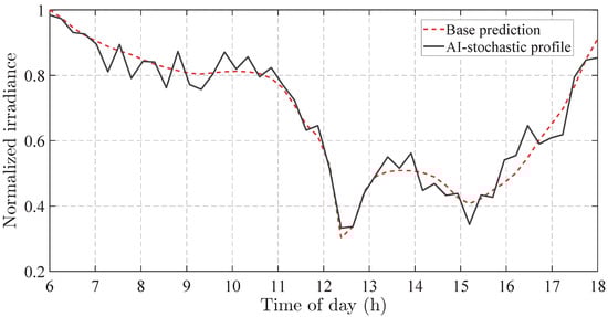
Figure 2.
Comparison of the base irradiance prediction and the AI-stochastic profile.
Studies have examined the impact of tilt angle and orientation (Figure 3, [20]) on PV performance; for this location, a tilt angle of 10° was used in the simulation. Deviations from the optimal configuration cause significant energy losses, especially in equatorial regions, where optimal annual angles vary by 5.1°. In addition, ambient temperature and increased irradiance significantly raise the module’s operating temperature, directly impacting its performance [21,22,23]. Therefore, simulations included ambient temperature variations, as they influence the actual power output of the photovoltaic system.
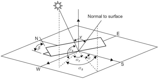
Figure 3.
Representation of orientation parameters: tilt and solar azimuth.
For the simulation, the DIgSILENT PowerFactory 2024 software was used, which includes a specialized photovoltaic model in which each unit represents a set of solar panels interconnected to the grid via a single inverter. The model can automatically estimate the active power setpoint using geographic location, date, and local time, enabling realistic, time-dependent power flow simulations. Now, within the PowerFactory simulation environment, the real power generated can be entered manually or automatically based on the PV module type, array configuration, simulation time (date and time), and irradiance levels. In general, the system’s total power is obtained by multiplying the nominal capacity of a single photovoltaic array by the number of inverters connected in parallel. Equation (1) determines system generation capacity from the module unit power and the number of modules per inverter [20].
where:
- represents the total active power of the photovoltaic system.
- is the active power generated by an individual panel.
- corresponds to the total number of panels connected to an inverter.
Table 1 shows the electrical parameters of the photovoltaic module used in the simulation. The photovoltaic module was manufactured in China. Each inverter was connected to the type of load associated with its corresponding node—single-phase, two-phase, or three-phase—so that the inverter connections accurately replicate the power supply scheme of the associated load, maintaining an adequate representation of the system’s behavior.

Table 1.
Technical parameters of the photovoltaic module considered in the simulation.
2.1. Quasi-Dynamic Simulation
Quasi-dynamic simulation is geared toward medium- and long-term electrical studies. This technique executes multiple load flows sequentially (here, unbalanced load flows) using predefined time steps. The analysis aims to represent long-term load and generation profiles and to simulate the network’s evolution over time. This method is computationally efficient because it avoids solving the full dynamic system equations, thus speeding up calculations. The quasi-dynamic method provides high fidelity and has been widely adopted in photovoltaic system studies; it accounts for time-varying generation and load, capturing fluctuations in electrical parameters over a defined period. As a result, the method is suitable for analyzing systems with PV sources, where generation varies according to irradiance and environmental conditions [24].
To perform the quasi-dynamic simulation, a full-day analysis period was selected, with a 30 min calculation interval between steps. This provides more detailed results on the system’s daily evolution. Reducing the step size could increase detail, but it is unnecessary, as it would prolong simulation time without significant analytical benefit.
2.2. Unbalanced Load Flow
As the basis for quasi-dynamic analysis, unbalanced load flow helps determine how the system’s behavior changes while maintaining the real operating conditions of a three-phase distribution network, despite phase imbalances. This method solves several load flows sequentially, changing photovoltaic injection and load at each step. Phase imbalances are common and must be included in load flow calculations for accuracy. EPS operating limits are set, and electrical parameters are determined via load flow. Many studies use numerical methods for load flow, with Newton–Raphson being the most popular due to its faster convergence compared to Fast Decoupled and Gauss–Seidel methods [25,26,27].
In unbalanced three-phase load flow analysis, the system is formulated from the relationship between injected currents and voltages, represented by the nodal admittance matrix (Equation (2)). This relationship is expressed in matrix form, accounting for the coupling between phases, as shown in (3). In it, the interactions between phases a, b, and c are modeled in each pair of nodes in the system [28].
where:
- : Vector of phase currents injected into node n
- : Vector of phase voltages at node n
- : Three-phase admittance matrix in phase coordinates
- : Vector of three-phase currents injected into the node
- : Vector of voltages at node j
- : Admittance matrix between nodes i and j
The current injected from phase p of bus i is obtained using Equation (4), which accumulates the effect of the voltages in all connected phases. Meanwhile, the complex power is represented according to (5), where the characteristic non-linearity of the problem is introduced.
where is the coupling between phases p and q at nodes i and k, and and correspond to the voltage and current in phase p of bus k.
The Newton–Raphson method was used as the power flow solver, due to its robustness and efficient convergence for distribution system studies. A convergence tolerance of 1 × 10⁻⁶ was applied throughout the simulation. The quasi-dynamic simulation process in PowerFactory is summarized in Algorithm 1, which describes the steps for modeling the load and photovoltaic generation profiles and performing an unbalanced load flow analysis at each time interval. The results allow for a comparative evaluation of the main electrical parameters in scenarios with and without photovoltaic integration.
| Algorithm 1 Quasi-Dynamic Simulation with High PV Penetration in PowerFactory |
|
3. Case Study
Two scenarios are proposed for analysis. In the first scenario, a quasi-dynamic simulation is performed, considering only hourly load variation, without PV generation. This scenario will serve as a basis for comparing the effects of incorporating PV generation into the system. In the second scenario, PV generation is added to the demand variations, modeled using hourly profiles of ambient temperature and local climatic conditions in Ecuador. This data represents the effect of clouds, providing a more realistic representation of energy production in the PowerFactory simulation environment. It is worth noting that the load power factor was maintained constant throughout the simulation.
Residential and commercial load profiles were simulated to represent hourly demand, as shown in Figure 4, illustrating typical daily consumption variations for each load type. Additional curves for the remaining loads were generated from these profiles, with a random deviation of ±8%.
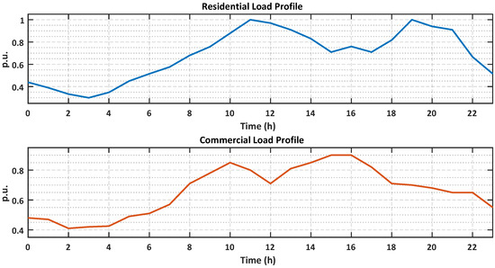
Figure 4.
Typical daily residential and commercial load profiles in per-unit values, showing that residential demand peaks around midday and in the evening, while the commercial profile exhibits a broader and sustained peak throughout working hours.
The simulations used the IEEE 13-node system, characterized by a radial configuration. The feeder includes 13 unbalanced loads and 10 sections, combining overhead lines and underground cables in single-, two-, and three-phase configurations. Additionally, it features two capacitor banks, a transformer, and a per-phase voltage regulator. This system was modified to analyze the impact of PV generation. For this purpose, PV generation was incorporated into the load nodes [29], as shown in Figure 5.
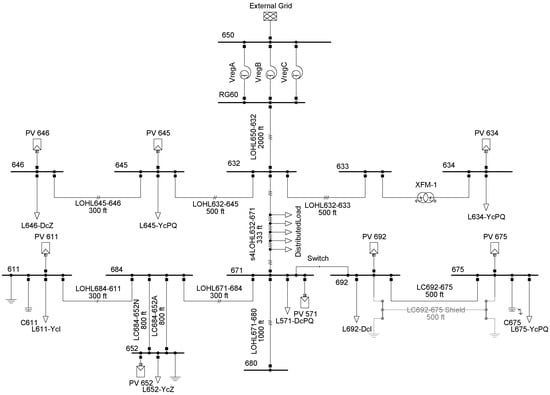
Figure 5.
Modified single-line diagram of the 13-node IEEE system with PV generation integration.
The two capacitor banks’ reactive power compensation was changed from fixed to quasi-dynamic, adjusting to connected loads to avoid overcompensation. In this way, the compensation level is adjusted according to instantaneous demand. On the other hand, the loads located at nodes 611, 634, 645, 646, 652, and 692 were defined as residential loads, as were the distributed loads located between nodes 632–671. In contrast, the largest loads at nodes 571 and 675 were classified as commercial based on their power ratings.
Table 2 summarizes the active and reactive power of loads in the IEEE 13-node system, including the load model and the power values for each of the three phases.
Table 2.
Real and reactive power of loads in the IEEE 13-node system.
Table 3 presents the installed capacity of the photovoltaic plants considered in the simulation. For each bus, the table provides the connection technology and the rated power in kilowatt-peak (kWp). These data serve as input parameters for the quasi-dynamic simulations.
Table 3.
Installed capacity of photovoltaic plants.
4. Results and Discussion
This section presents a detailed analysis of the results from the quasi-dynamic simulations. The study was conducted on a computer with a 12th-generation Intel Core i5 processor, 8 GB of RAM, and a 64-bit version of Windows 10.
Figure 6 shows the hourly generation profile of the external grid in the presence of photovoltaic power injection over a typical day. It can be seen that the interval of highest solar irradiance occurs between 10:00 a.m. and 12:00 p.m. During this time, photovoltaic generation reached a maximum value of 2711 kW, representing approximately 86% of instantaneous demand. In terms of energy balance, the photovoltaic system achieved a total daily production of 17,626 kWh. In comparison, the total energy demand recorded was 55,720 kWh, indicating that PV generation accounted for 31.6% of the demand, a significant contribution to the system’s supply.
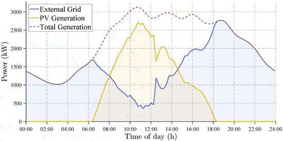
Figure 6.
Impact of PV generation on the external grid demand profile, showing an inverse relationship where increased PV output during daylight hours reduces the power drawn from the external grid.
The daily profile of active and reactive power delivered by the external grid is shown in Figure 7, which indicates a gradual reduction in active power between 8:00 a.m. and 3:00 p.m. due to the increased participation of photovoltaic generation during that interval. Furthermore, during the hours of highest irradiation, photovoltaic generation reduces the active power requirement from the grid, leading to reactive power demand exceeding active power demand.
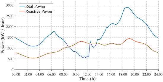
Figure 7.
Hourly profile comparison of real power and reactive power drawn from the external grid.
4.1. Voltage Profile Analysis
Figure 8 shows a comparison of the voltage magnitude at each node, with the phase having the highest magnitude at the point of maximum irradiance used as a reference. The dashed line serves as a visual reference for the 1 p.u. value, aiding in the interpretation of the figure. The location of the PV panels helps to reduce voltage drops in areas far from the main node (650), as seen in nodes 611 and 652, where voltage levels were initially below 0.98 and 0.99 p.u., and improved with PV integration. However, nodes 671, 675, and 692, which already had overvoltages, experienced further increases, reaching levels close to 1.07 p.u. In addition, nodes near the transformer (such as node 632) and those with low local demand (nodes 645 and 646) showed an increase in voltage close to the maximum threshold of 1.05 p.u., reaching the upper limit recommended by power quality standards [30].
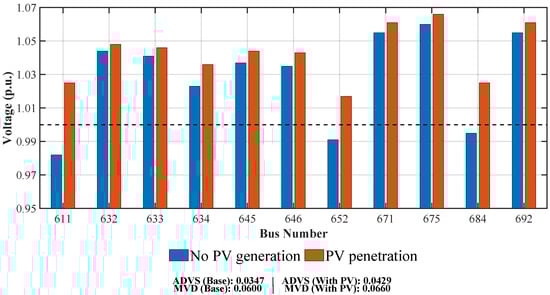
Figure 8.
Comparison of voltage magnitude across selected buses under two scenarios: No PV generation (base) and during peak solar penetration.
The results show that distributed PV integration in the IEEE 13-node system significantly affects voltage profiles. As shown in Figure 8, PV installation helps mitigate voltage drops in nodes far from the main bus. Conversely, nodes already experiencing overvoltages showed further increases, reaching nearly 1.07 p.u. Similar behavior has been reported in previous studies [29], where PV integration at load buses mitigated voltage drops at the ends of radial feeders while increasing voltage at buses with low local demand or near transformers. Furthermore, Ref. [14] also highlights that a high penetration of photovoltaic systems can have serious implications for the stability and reliability of electrical networks. These findings indicate that, although distributed PV can improve voltage levels in under-voltage nodes, careful siting and sizing are required to avoid overvoltage conditions.
The analysis of the voltage profiles is performed using Equation (6) to calculate the average voltage deviation throughout the system and Equation (7) to calculate the maximum voltage deviation [31].
The results show that the in case 2 is close to 0.05 per unit during peak FV penetration. On the other hand, the in bus 675 increases from 0.06 to 0.066 per unit, which is well above the recommended nominal value.
The daily profile for the base and PV injection scenarios is shown in Figure 9, with a peak overvoltage around 9:00–11:00 a.m. and a trough at midday (minimum 0.98 p.u. in the initial case). However, in the second case, it increases significantly in nodes 611, 634, 646, and 675, reaching values of up to 1.07 per unit.
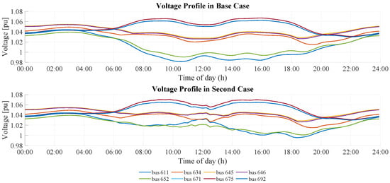
Figure 9.
Comparison of the daily voltage profile across multiple buses for the base case and the PV scenario, where the introduction of PV power generally raises the voltage magnitude across all buses throughout the day.
4.2. Voltage Imbalance
IEEE Std 1159-2019 [30] is the Recommended Practice for Monitoring Electric Power Quality, providing definitions, summaries, and characterizations of typical power quality phenomena in electrical systems. According to this standard, voltage imbalance in a three-phase system is typically less than 5% in low-voltage networks. Minor voltage imbalance (below 2%) is mainly caused by unbalanced single-phase loads, while severe voltage imbalance (above 5%) can occur under single-phasing conditions. Considering that the IEEE 13-node test system operates at medium voltage, a conservative limit of 3% is adopted in the simulations to represent realistic operating conditions and assess the impact of distributed PV generation.
The percentage of voltage imbalance is calculated using the positive and negative sequence components according to Equation (8), which allows the degree of asymmetry in the three-phase system to be quantified for evaluating electrical power quality [30,32,33].
where and correspond to the negative and positive sequence components of the voltage on bus k, respectively.
Figure 10 shows the behavior of voltage imbalance during maximum irradiance, both in the base case and in the PV penetration case. Nodes 632 and 633 initially record imbalance values of approximately 0.6%, whereas with PV generation, these increase to 0.72%. It should be noted that nodes such as node 634 are far from the reactive compensation zone, which is located at nodes 611 and 675.
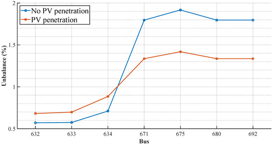
Figure 10.
Comparison of the voltage imbalance index across various buses, highlighting the impact of PV penetration.
Starting with bus 671, the imbalance initially reaches values close to the IEEE Std 1159-2019 reference limit. However, integrating PV generation reduced voltage imbalance, with improvements of up to 74% at nodes 671, 675, 680, and 692. This behavior indicates that PV generation improves voltage symmetry and reduces the presence of negative-sequence components. It is worth noting that the nodes not shown in the graph correspond to connection points with single-phase or two-phase loads, for which imbalance evaluation is not applicable.
4.3. Power Factor at the Nodes
The power factor indicates the efficiency with which active power is used relative to the total power delivered. Figure 11 shows the average PF values in the two scenarios, where the main node 650 has a PF of 0.903 p.u. in the initial case; however, during PV generation, this value is reduced to 0.819 per unit. This change is due to the decrease in the active component of the external source, resulting from the contribution of local generation, as reactive power is not compensated in the same proportion. Nodes 632, 633, and 684 are transfer nodes, which is why they have the lowest PF.
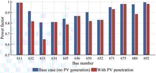
Figure 11.
Comparison of the average power factor across selected buses for the base case and with PV penetration, showing that PV integration generally reduces the system PF.
When performing an hourly analysis of the power factor at the main node, it is observed that the peak hours of PV generation (between 10:00 a.m. and 12:00 p.m.) coincide with a decrease in the power factor, reaching a minimum of 0.35 inductance. However, in Ecuador, Arconel Resolution 005/18 sets a minimum power factor of 0.92 for the primary grid. Therefore, to improve this condition, reactive power compensation is performed at the main node using a capacitor bank, adjusting the compensator tap in the quasi-dynamic simulation. Figure 12 shows the behavior of the power factor throughout the day for the base case, solar generation, and reactive power compensation.
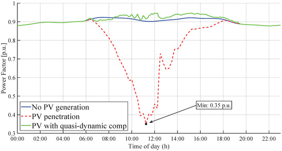
Figure 12.
Daily PF variation at the main node (bus 650), showing that PV penetration significantly reduces the PF during daylight hours.
4.4. Line Loadability
Figure 13 shows the load capacity of the lines. With the integration of PV generation, there is an improvement in the loadability of the lines during the hours of highest PV injection, especially between 9:00 a.m. and 4:00 p.m., when, on several links such as 650–632, 692–675, and 632–645, the load capacity decreases by up to 60%.
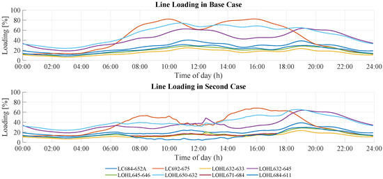
Figure 13.
Comparison of the daily line loading percentage across critical lines for the base case and with PV generation.
5. Conclusions
The analysis reveals that high penetration of PV systems in distribution networks impacts the electrical grid in multiple ways. At low solar penetration (morning and afternoon), the voltage profile generally improves. However, when certain integration levels are exceeded, voltage limits are violated (Figure 9). PV generation also enhances voltage symmetry, keeping it within the limits recommended by IEEE Std 1559-2019. Deviation metrics (Equations (6) and (7)) indicate that system voltage, both on average and in maximum deviation, tends to increase to values close to 0.05 p.u. () and 0.066 p.u. (), exceeding thresholds established by power quality standards.
PV integration produces asymmetric impacts during maximum irradiance (Figure 8), reducing voltage drops at distant nodes (611, 652) while generating overvoltages near capacitor banks (671, 675, 692), reaching up to 1.07 p.u. These results highlight the need for careful PV placement and sizing to prevent local overvoltages.
Additionally, the power factor at the main node (650) decreases from 0.903 to 0.819 p.u. (Figure 11), reaching a minimum of 0.35 p.u. during peak PV generation. This reduction exceeds the Ecuadorian regulatory limit (ARCONEL Resolution 005/18) and is caused by the imbalance between reduced external active power and increased uncompensated reactive power. Installing a capacitor bank at the main node corrects the power factor to meet regulatory limits (Figure 12), supporting network operators in managing voltage quality and system performance.
Regarding line loading, capacity reductions of up to 60% were observed on lines 650–632, 692–675, and 632–645, which helps decongest the network and reduce energy losses. However, these findings are subject to limitations, including the simplified network model, assumptions on load profiles, and PV generation variability. Load distribution and the location of PV systems significantly influence potential network overloads. Additionally, the results can be affected by the simulation date, as DIgSILENT PowerFactory accounts for temporal variations, as well as environmental conditions such as temperature and cloud cover. Optimizing PV placement is recommended to ensure safe and reliable operation under high photovoltaic penetration.
Author Contributions
Conceptualization, E.G.; Methodology, J.V.; Formal analysis, D.C.; Data curation, A.Á.; Writing original draft, J.V. and E.G.; Writing review and editing, D.C. and A.Á.; Supervision, D.C.; Project administration, D.C.; Funding acquisition, D.C. All authors have read and agreed to the published version of the manuscript.
Funding
Salesian Polytechnic University and GIREI-Smart Grid Research Group supported this work.
Data Availability Statement
The original contributions presented in this study are included in the article. Further inquiries can be directed to the corresponding author.
Conflicts of Interest
The authors declare no conflicts of interest.
References
- Ministerio de Energia y Minas. Plan Maestro de Electricidad 2023–2032; Technical Report; CENACE: Quito, Ecuador, 2024. [Google Scholar]
- Operador Nacional de Electricidad—CENACE. Información Operativa en Tiempo Real. 2024. Available online: https://www.cenace.gob.ec/info-operativa/InformacionOperativa.htm (accessed on 29 August 2025).
- Mourad Mabrook, M.; Donkol, A.A.; Mabrouk, A.M.; Hussein, A.I.; Barakat, M. Enhanced the Hosting Capacity of a Photovoltaic Solar System Through the Utilization of a Model Predictive Controller. IEEE Access 2024, 12, 62480–62491. [Google Scholar] [CrossRef]
- Sánchez Oñate, P.S. Estabilidad De Frecuencia En Sistemas Eléctricos De Potencia Considerando Generación No Inercial. Univ. Politec. Sales. QUITO 2020, 1, 134. [Google Scholar]
- Wu, S.; Yang, P.; Zhang, Y.; Gao, D.; Li, C.; Liu, F. On the Key Factors of Frequency Stability in Future Low-Inertia Power Systems. In Proceedings of the 2020 2nd International Conference on Smart Power & Internet Energy Systems (SPIES), Bangkok, Thailand, 15–18 September 2020; pp. 240–245. [Google Scholar] [CrossRef]
- Munkhchuluun, E.; Meegahapola, L.; Vahidnia, A. Reactive Power Control of PV for improvement of Frequency Stability of Power systems. In Proceedings of the 2020 IEEE Power & Energy Society General Meeting (PESGM), Montreal, QC, Canada,, 2–6 August 2020; pp. 1–5. [Google Scholar] [CrossRef]
- Nwaigwe, K.; Mutabilwa, P.; Dintwa, E. An overview of solar power (PV systems) integration into electricity grids. Mater. Sci. Energy Technol. 2019, 2, 629–633. [Google Scholar] [CrossRef]
- Kiangebeni Lusimbakio, K.; Boketsu Lokanga, T.; Sedi Nzakuna, P.; Paciello, V.; Nzuru Nsekere, J.P.; Tshimanga Tshipata, O. Evaluation of the Impact of Photovoltaic Solar Power Plant Integration into the Grid: A Case Study of the Western Transmission Network in the Democratic Republic of Congo. Energies 2025, 18, 639. [Google Scholar] [CrossRef]
- Marin, C.; Mendes, M.A.; Batista, O.E. Estudo da estabilidade de tensão em sistemas de distribuição com alta penetração de geração distribuída. In Proceedings of the XXIII Congresso Brasileiro de Automática (CBA), Porto Alegre, Brazil, 23–26 November 2020. [Google Scholar]
- Mitra, P.; Heydt, G.T.; Vittal, V. The impact of distributed photovoltaic generation on residential distribution systems. In Proceedings of the 2012 North American Power Symposium (NAPS), Champaign, IL, USA, 9–11 September 2012; pp. 1–6. [Google Scholar]
- Yan, R.; Saha, T.K. Investigation of Voltage Stability for Residential Customers Due to High Photovoltaic Penetrations. IEEE Trans. Power Syst. 2012, 27, 651–662. [Google Scholar] [CrossRef]
- Kharrazi, A.; Sreeram, V.; Mishra, Y. Assessment techniques of the impact of grid-tied rooftop photovoltaic generation on the power quality of low voltage distribution network—A review. Renew. Sustain. Energy Rev. 2020, 120, 109643. [Google Scholar] [CrossRef]
- Rakhshani, E.; Rouzbehi, K.; Sánchez, A.J.; Tobar, A.C.; Pouresmaeil, E. Integration of Large Scale PV-Based Generation into Power Systems: A Survey. Energies 2019, 12, 1425. [Google Scholar] [CrossRef]
- Gandhi, O.; Kumar, D.S.; Rodríguez-Gallegos, C.D.; Srinivasan, D. Review of power system impacts at high PV penetration Part I: Factors limiting PV penetration. Sol. Energy 2020, 210, 181–201. [Google Scholar] [CrossRef]
- Ismail, B.; Wahab, N.I.A.; Othman, M.L.; Radzi, M.A.M.; Vijayakumar, K.N.; Rahmat, M.K.; Naain, M.N.M. New Line Voltage Stability Index (BVSI) for Voltage Stability Assessment in Power System: The Comparative Studies. IEEE Access 2022, 10, 103906–103931. [Google Scholar] [CrossRef]
- Zhou, Y.; Xu, T.; Ye, L.; Liu, M.; Chen, X.; Yang, Y.; Guo, Q.; Sun, H. Transient Rotor Angle and Voltage Stability Discrimination Based on Deep Convolutional Neural Network with Multiple Inputs. In Proceedings of the 2021 IEEE 4th International Electrical and Energy Conference (CIEEC), Wuhan, China, 28–30 May 2021; pp. 1–6. [Google Scholar] [CrossRef]
- He, Q.; Qi, F.; Wang, S.; Zeng, Y.; Sheng, H.; Ma, J. Research on Static Voltage Stability Index of Regional Power Network with New Energy Stations Based on Voltage Stability Criterion. In Proceedings of the 2023 IEEE 7th Conference on Energy Internet and Energy System Integration (EI2), Hangzhou, China, 15–18 December 2023; pp. 2597–2601. [Google Scholar] [CrossRef]
- Hao, W.; Chen, M.; Gan, D. Short-Term Voltage Stability Analysis and Enhancement Strategies for Power Systems With Photovoltaic Penetration. IEEE Access 2024, 12, 88728–88738. [Google Scholar] [CrossRef]
- Cai, L.J.; Erlich, I. Power system static voltage stability analysis considering all active and reactive power controls—Singular value approach. In Proceedings of the 2007 IEEE Lausanne POWERTECH, Lausanne, Switzerland, 1–5 July 2007; pp. 367–373. [Google Scholar] [CrossRef]
- Kyrylenko, O.; Denysiuk, S.; Strzelecki, R.; Blinov, I.; Zaitsev, I.; Zaporozhets, A. Studies in Systems, Decision and Control 512. In Power Systems Research and Operation Selected Problems III; Springer: Cham, Swizerland, 2023. [Google Scholar]
- Jamal, J.; Mansur, I.; Rasid, A.; Mulyadi, M.; Dihyah Marwan, M.; Marwan, M. Evaluating the shading effect of photovoltaic panels to optimize the performance ratio of a solar power system. Results Eng. 2024, 21, 101878. [Google Scholar] [CrossRef]
- Barbón, A.; Bayón-Cueli, C.; Bayón, L.; Rodríguez-Suanzes, C. Analysis of the tilt and azimuth angles of photovoltaic systems in non-ideal positions for urban applications. Appl. Energy 2022, 305, 117802. [Google Scholar] [CrossRef]
- Mukisa, N.; Zamora, R. Optimal tilt angle for solar photovoltaic modules on pitched rooftops: A case of low latitude equatorial region. Sustain. Energy Technol. Assessments 2022, 50, 101821. [Google Scholar] [CrossRef]
- Gaitan, L.; Gomez Ariza, J.; Rivas, E. Quasi-Dynamic Analysis of a Local Distribution System with Distributed Generation. Study Case: The IEEE 13 Node System. TecnoLógicas 2019, 22, 195–212. [Google Scholar] [CrossRef]
- Afolabi, O.A.; Ali, W.H.; Cofie, P.; Fuller, J.; Obiomon, P.; Kolawole, E.S. Analysis of the Load Flow Problem in Power System Planning Studies. Energy Power Eng. 2015, 7, 509–523. [Google Scholar] [CrossRef]
- Stott, B. Review of load-flow calculation methods. Proc. IEEE 1974, 62, 916–929. [Google Scholar] [CrossRef]
- Irving, M.; Sterling, M. Efficient Newton-Raphson algorithm for load-flow calculation in transmission and distribution networks. IEE Proc. C (Generation, Transm. Distrib.) 1987, 134, 325–330. [Google Scholar] [CrossRef]
- Sereeter, B.; Vuik, K.; Witteveen, C. Newton Power Flow Methods for Unbalanced Three-Phase Distribution Networks. Energies 2017, 10, 1658. [Google Scholar] [CrossRef]
- Shinde, K.D.; Mane, P.B. Investigation of Effects of Solar Photovoltaic Penetration in an IEEE 13-bus Radial Low-Voltage Distribution Feeder System. In Proceedings of the 2022 19th International Conference on Electrical Engineering/Electronics, Computer, Telecommunications and Information Technology (ECTI-CON), Prachuap Khiri Khan, Thailand, 24–27 May 2022; pp. 1–5. [Google Scholar] [CrossRef]
- IEEE Std 1159-2019 (Revision of IEEE Std 1159-2009); IEEE Recommended Practice for Monitoring Electric Power Quality. IEEE: New York, NY, USA, 2019; pp. 1–98. [CrossRef]
- Ortiz, L.; Orizondo, R.; Águila, A.; González, J.W.; López, G.J.; Isaac, I. Hybrid AC/DC microgrid test system simulation: Grid-connected mode. Heliyon 2019, 5, e02862. [Google Scholar] [CrossRef] [PubMed]
- Beneteli, T.A.; Cota, L.P.; Euzébio, T.A. Limiting current and voltage unbalances in distribution systems: A metaheuristic-based decision support system. Int. J. Electr. Power Energy Syst. 2022, 135, 107538. [Google Scholar] [CrossRef]
- Nacar Cikan, N.; Cikan, M. Reconfiguration of 123-bus unbalanced power distribution network analysis by considering minimization of current & voltage unbalanced indexes and power loss. Int. J. Electr. Power Energy Syst. 2024, 157, 109796. [Google Scholar] [CrossRef]


Disclaimer/Publisher’s Note: The statements, opinions and data contained in all publications are solely those of the individual author(s) and contributor(s) and not of MDPI and/or the editor(s). MDPI and/or the editor(s) disclaim responsibility for any injury to people or property resulting from any ideas, methods, instructions or products referred to in the content. |
© 2025 by the authors. Licensee MDPI, Basel, Switzerland. This article is an open access article distributed under the terms and conditions of the Creative Commons Attribution (CC BY) license (https://creativecommons.org/licenses/by/4.0/).